1
Università di Pisa
Facoltà di Ingegneria
Corso di Laurea Magistrale in Ingegneria Elettronica
Final work
Design and FPGA implementation
of a fast clustering algorithm for
satellite lightning imaging applications
Session 2012/2013
Nominee: Andrea Lampredi
Supervisors: Prof. Ing. Luca Fanucci
………
………
Ing. Daniele Davalle
2
Summary
Chapter 1 Meteorological satellites ... 7
1.1 Satellite orbit... 7 1.1.1 GEO ... 8 1.1.2 LEO ... 9 1.1.3 Polar orbit ... 10 1.1.4 MEO ... 11 1.1.5 HEO ... 11
1.2 History of meteorological satellites ... 12
1.3 EUMETSAT ... 13
1.4 Meteosat First Generation (MFG) ... 15
1.4.1 MFG characteristics ... 16
1.4.2 MVIRI ... 17
1.5 Meteosat Second Generation (MSG) ... 19
1.5.1 Radiometer SEVIRI ... 21
1.5.2 Radiometer GERB ... 27
1.6 Meteosat Third Generation (MTG) ... 29
1.6.1 MTG-S ... 31
1.6.2 MTG-I ... 34
Chapter 2 Lightning Imager ... 37
2.1 Image capture ... 41
2.2 Noise rejection ... 44
2.3 Background removal and adaptive threshold ... 46
2.4 Events detection and on-board processing for FEs ... 49
2.5 Information addition ... 52
2.6 Conversion DT – data ... 52
Chapter 3 Clustering algorithm ... 54
3
3.2 Definitions ... 61
3.3 Functional requirements ... 63
3.3.1 Cluster Window ... 63
3.3.2 Window number minimization ... 64
3.3.3 Window overlap ... 65
3.3.4 Algorithm throughput ... 66
3.3.5 Output data format ... 66
3.4 Algorithm implementation ... 66
3.5 Algorithm optimization ... 70
3.6 MATlab High level model ... 75
3.6.1 Expansion strategies ... 75
3.6.2 Test-vector generation ... 77
3.6.3 High-level model ... 80
3.7 Bit-true MATlab model ... 87
3.7.1 Adjacency Check ... 89
3.7.2 P_Window Check ... 91
3.7.3 Candidate Window Selection ... 92
3.7.4 Expandability Check ... 93
3.7.5 Priority Selection ... 102
3.7.6 Window update ... 102
3.7.7 Add neighbors ... 103
3.7.8 MATlab main code ... 104
3.7.9 Results ... 105
3.8 From MATlab bit-true to VHDL model ... 110
3.8.1 Adjacency Check ... 115
3.8.2 P_Window Check ... 117
3.8.3 Candidate Window Selection ... 118
3.8.4 P_Window Selection ... 120
4 3.8.6 Priority Selection ... 121 3.8.7 Window update ... 122 3.8.8 Add Neighbors ... 122 3.8.9 RAM memory ... 123 3.8.10 Window Load ... 124
3.8.11 Global State Machine ... 126
3.9 Algorithm optimization ... 127
3.9.1 Window Load and RAM block ... 128
3.9.2 AC_CWS branch ... 129
3.9.3 PWC_PWS branch ... 132
3.9.4 Expandability Check optimization... 134
3.9.5 PS and WU ... 136
3.9.6 Add Neighbors ... 136
3.9.7 Global State Machine ... 137
3.9.8 Global top level ... 141
3.9.9 Timing analysis ... 143
Chapter 4 Conclusion ... 147
5
Thanks
Desidero dal profondo del cuore ringraziare tutte le persone che mi hanno aiutato ad arrivare a questo momento così fortemente voluto da sempre ma che all’inizio sembrava solamente una chimera.
Primi tra tutti i miei genitori e mio fratello, che mi hanno sempre sostenuto e sopportato nei momenti difficili e mi hanno donato la forza per non arrendermi mai. Hanno ascoltato le mie sfuriate, hanno passato anni a consolarmi e hanno riso e pianto con me, sempre.
Tutta la mia famiglia che mi ha visto tante volte uscire vittorioso ma a volte anche sconfitto.
La mia splendida fidanzata che ha reso facili e piacevoli tutti i momenti più difficili, che mi ha fatto tornare il sorriso anche dopo tuffi profondi e ha permesso che questa tesi arrivasse alla fine con la sua grandissima intelligenza e disponibilità.
I miei compagni di università che hanno fatto in modo di trasformare questi anni di università in una bellissima esperienza da vivere a pieni polmoni.
I miei compagni di squadra che, forse, hanno notato solo la parte più distruttiva del mio lavoro vedendo spesso, sulla mia faccia, la stanchezza di giornate passate sui libri ma che, nonostante tutto, mi hanno sempre permesso di ricaricare le pile.
I miei amici che mi ha sempre incoraggiato in tutto quello che facevo.
I professori che mi hanno seguito e mi hanno permesso di diventare quello che sono adesso.
6
Introduction
This thesis deals with the implementation of a new kind of clustering algorithm that will be used by a Lightning Imager (LI) mounted on ESA meteorological satellites of third generation (MTG). The development of this algorithm is commissioned to the Department of Information Engineering by Selex ES in cooperation with ESA (European Space Agency). At first, the algorithm is designed to meet the stringent timing requirements. Then, the new clustering algorithm is implemented on MATlab and VHDL languages.
The thesis is organized as follows:
Chapter 1, Meteorological satellites, introduces the principal orbits used by every kind of satellite, the data provided by meteorological missions and the history - past, present and future - of meteorology. A particular section is reserved to EUMETSAT and its missions with a large presentation of EUMETSAT three generations of satellites:.
o Meteosat First Generation series. A short resume of history, position, lifetime and technical data with a particular section dedicated to the principal instrument on board, the MVIRI;
o Meteosat Second Generation, the active series in orbit around the Earth. It gives details about satellite principal instruments, SEVIRI and GERB, and their characteristics; o Meteosat Third Generation. A presentation about the new MTG series that will be soon
in orbit. It explains which instrument will be on board and which characteristics they will have. Also, the difference between MTG-I and MTG-s will shown;
Chapter 2, Lightning Imager, exposes what is an imager and the requirements necessary to implement this device. Then, it presents the problems during the capturing and which methods are used to increase the quality of events detection;
Chapter 3 is focused on the LI technology and his most important parts: requirements will be analyzed and their feasibility will be evaluated. The next step is the design of the clustering algorithm and the work will be concluded with three output codes: a MATlab High-Level (MHL) model, a MATlab Bit-True (MBT) model and a prototype of VHDL model for hardware implementation.
7
Chapter 1
Meteorological satellites
In the modern meteorology, the satellites have several and fundamental functions: thanks to their continuous presence in orbit around the Earth, the weather is always monitored to find new meteorological phenomena. Furthermore, these satellites can pick up a lot of data about temperature, wind, NOx gas, pollution, both on land and sea. Then, this great quantity of data is sent to the ground
stations: they provide weather previsions (with model of meteorological forecast), update conditions about Ozone hole, Earth’s pollution and many other applications..
1.1 Satellite orbit
Satellites can work on several orbits and the orbit depends on the kind of mission.
8
The orbits for satellites of commercial telecommunication's missions are usually GEO (Geostationary Earth Orbit) but, recently, there are some new satellites on LEO (Low Earth Orbits) and inclined orbit. On the other hand, meteorological satellites use geostationary and polar orbits. There are also many different possible orbits like MEO (Medium Earth Orbits) or HEO (Highly Elliptical Orbits).
In the following, a classification and a description of the different meteorological satellite orbits are presented.
1.1.1 GEO
The Geostationary Earth Orbit (GEO) was introduced in 1945: Arthur C. Clarke, a lieutenant of Royal Air Force (RAF), published a work (“Extraterrestrial Relays”) on the English magazine “Wireless World” in which he talked about artificial satellites in orbit around the Earth [1]. He proposed only 3 satellites, synchronous with Earth rotation (geostationary), which can be used like “radio gate” in the space and have warranted communication for the whole planet.
Today, Geostationary satellites orbit on 35800 km around the Earth: this height is called “Geostationary orbit” because the time of revolution around the Earth is identical to the time of Earth's rotation (23 hours, 56 minutes and 4 seconds); so they are stationary relative to the surface (satellites rotate in the same direction of Earth’s rotation). This type of satellites is also called geosynchronous. This is why this kind of satellites is usually used for meteorological forecasts: at 35800 km, a single satellite can scan about a third of all surface and it can continuously follow atmospheric phenomena like cyclones and hurricanes. Furthermore, geostationary satellites are usually used for device which have point-to-point or broadcasting communication because antennas of these devices are simple and fixed to the same direction: they don’t need a continuous calibration towards the satellite.
Figure 1.2: Revolution period around the Earth of geostationary satellite.
5 satellites are needed in order to cover all the Earth’s surface. At the moment, there are lots of geostationary satellites [2]:
9 METEOSAT for Europe;
GOES for USA; MTSAT for Japan; Fengyun-2 for China; GOMS for Russia; KALPANA for India.
A geostationary orbit must stay on the same plane of the Equator; so satellites have a decreasing view towards poles. Polar and sub-polar area are difficultly covered by this kind of satellites because antennas could be pointed under the horizon line.
Typical parameters of GEO:
Height above equator: 35,786 km;
Orbit radius: 42,155 km (Orbit circumference: 264,869 km); Orbital velocity: 11,066 km/h = 3.07 km/s;
Latitude coverage: between 75° North to 75° South.
As already mentioned, GEO satellites have significant advantages: just 5 GEO satellites are sufficient to cover all the communication on the planet. In addition, GEO satellites have a fixed position relatively to the Earth surface, which eases the satellite pointing for ground devices.
This orbit has also some cons. First of all, satellites on this orbit need expensive missions for their launch, because of the high distance from the surface. They usually use multistage launcher (often Ariane vehicles were used in the past for these missions, [21] ) . Moreover, the propagation of radio waves has high delay, 0.12 seconds, still due to the high satellite distance. This delay is satisfactory for broadcast communication but hardly sufficient in telephone communication.
1.1.2 LEO
When a satellite orbit around the Earth at an altitude up to 2000 km, the orbit is called “Low Earth Orbit” (LEO). Typically, LEO’s satellites work between 300 and 800 km. Under 300 Km, because of high density of gasses in atmosphere, the high friction against them decelerate the satellite resulting in a fast orbital decay. Too much energy (high velocity) is necessary to maintain the satellite in orbit. Above 2000 Km, there is the “Van Allen belt” (an area full of free charges held together by the Earth’s magnetic field) which can provoke malfunction in the electronic circuits on board due to the high exposition to radiations [1].
10
As defined by Keplero’s laws, LEO’s satellites orbit near the planet with very high velocity, about 30000 Km/h, and make a full revolution around Earth in 90 minutes. Almost all of space voyagers had place in low orbit and the spatial station stay, even today, in this orbit too (Saljut, MIR and International Space Station, [20]).
Compared to GEO satellites, LEO’s satellites orbit near the surface: it allows communication with low delay (20–25 ms, like some terrestrial communication) so they are used for remote sensing and military missions. Furthermore, the cost of LEO’s launch is cheaper than GEO’s launch. LEO’s satellites are also suitable for the communication with the surface: low distance allows low power and simple antenna for communication.
On the other hand, low orbit has many cons. First of all, LEO’s satellite are visible by the ground station only for few minutes over the horizon and, during this time, it’s very fast. The rest of time, the satellite is useless for that station. Obviously, because of his velocity, the ground station antenna must be oriented every time towards satellite in order to maintain the communication. Moreover, the communication is affected by an high Doppler effect: this effect must be compensated automatically by electronic circuits on board but they increase the complexity of the satellite’s system.
In the past, LEO satellites were almost unused because of their short view time, but recently they are largely used thanks to the high number of in-orbit satellites on several orbital planes: today, with about 100 satellites the planet is fully covered and communication is continuously allowed.
LEO satellites are used mainly for mobile telephone with full planet’s coverage like Globalstar or Iridium.
If the orbit of these systems is very inclined, it becomes polar orbit.
1.1.3 Polar orbit
Polar satellites orbit around Earth at an altitude of 800 km. A single satellite stays on the same area of surface for only twice a day: more than one satellite and a system of coordination between them are needed for meteorological observation. At the moment, meteorological satellites on polar orbit are [2] :
METOP by EUMETSAT for Europe; NOAA and QuikSCAT for USA; Meteor for Russia;
11
Polar satellites guarantee a better vision of planet than GEO’s satellites: polar satellites can observe even polar areas and that’s why they are used for missions of remote sensing and surveillance.
Polar satellites have orbits inclined of about 90 degrees with respect to the Equator plane and, usually, they are sun-synchronous, i.e., (the same area is scanned by the same satellite at the same moment of the day, during every season). Therefore, while the satellite scans from North to South on his orbit, the planet makes his rotation orbit and the result is that satellite scans all the surface, step by step. Because of these characteristics, polar satellites are perfect to scan the evolution of meteorological phenomena in the same condition and compare these for long time periods.
Figure 1.3: Full disc scan by polar orbit.
1.1.4 MEO
The “Medium Earth Orbit” (MEO) is a circular orbit at an altitude of about 10000 Km. Their orbital period is about 6 hours and the maximum period of over-horizon time is about some hours; with 10-12 satellites (on 2-3 orbit planes) the planet is fully covered. The most famous system based on MEO is the Global Positioning System (GPS), a system for accurate positioning on the planet surface.
1.1.5 HEO
The “Highly Elliptical Orbit” (HEO) was used for the first time by Russia to create communication with sub-polar zones which are isolated for GEO’s satellites. HEO have three geometrical characteristics:
Perigee, the lowest altitude point in the orbit, at about 500 km; Apogee, the highest altitude point in the orbit, at about 50000 km; Elliptic orbit at 63.4 degrees with respect to Equator.
12
In HEO, Earth stays in one of the two foci of the elliptical path. For this reason, the satellite stays for two third of its period near the Apogee: so, with a right positioning of the Apogee point, the area of interest can be rightly covered. Obviously, when the satellite is on the Perigee, the coverage of the affected zone is not guaranteed: so, more satellites are needed for a sufficient coverage, all together on the same orbit and with an accurate time distance. An example of this orbit is the system Molniya, used to cover Siberia. HEO has the same cons of GEO and LEO: for high distance (Apogee), communication have high delay and need high power (like GEO) and, for the high velocity, there is an high Doppler effect (like LEO).
1.2 History of meteorological satellites
The first satellites in the world, Sputnik, was sent by Russia in 1959 but it didn’t have meteorological instrument on board. The first satellite with meteorological instruments on board was Vanguard-2, in 1959. This satellite, by NASA, was destroyed during the first part of mission, so its data was not available. First images of the Earth were transmitted in 1960 by TIROS-1 (Television and Infra Red Observation Satellite), again by NASA: this satellite had two cameras and was used for only 78 days. These kinds of satellites have become important since 1961, when images of the hurricane “Carla” helped to save a lot of people in Gulf of Mexico.
In 1964 the first satellite of Nimbus series, Nimbus-1, introduced some news about technology: it was the first satellite stable on all the 3 axes, so it could point always towards the same direction, and it was the first polar sun-synchronous satellite.
In 1969, Russia started its meteorological satellites program and, in the same year, Nimbus-9 was sent in orbit: this satellite had on board measure’s instruments to pick up data about temperature, pressure, wetness..
In 1974 USA sent its first GEO’s satellite, SMS-1 (Synchronous Meteorological Satellite), and, in 1977-1978, also Europe and Japan sent their first GEO’s satellite (Meteosat for Europe and GMS, Geostationary Satellite Meteorological, for Japan). With Meteosat-1, some wavelengths, typical of water vapor (6.7 mm), were analyzed for the first time. In the 80’s, also India sent its first GEO’s satellite: with this one, the planet was fully covered and meteorological data were available 24/24 hours.
Now, the research will be focused about forecasting over European continent and about European missions in the past, in present day and in the future. First of all, it is necessary to know which organization is responsible of European meteorological missions.
13
1.3 EUMETSAT
EUMETSAT [3] (European Organization for the Exploitation of Meteorological Satellites) is an international organization created in 1986 to handle European meteorological satellites. The organization manages launch and control of satellites and their data transmission for meteorological and climate conditions. EUMETSAT is composed by 27 European states: Austria, Belgium, Croatia, Czech Republic, Denmark, Estonia, Finland, France, Germany, Greece, Hungary, Ireland, Italy, Leetonia, Luxemburg, Norway, Netherland, Poland, Portugal, UK, Romania, Slovakia, Slovenia, Spain, Sweden, Switzerland, Turkey. Also EUMETSAT has cooperation accord with Bulgaria, Iceland, Lithuania and Serbia.
Figure 1.4: EUMETSAT members and country cooperating. █ █ Member states.
█ █ Cooperation accord states.
As already said in the Sections 1.1.1 and 1.1.3, EUMETSAT’s meteorological satellites are of two kinds: geostationary (Meteosat) and polar (Metop). Other similar satellites are handled by NOAA, the USA agency; EUMETSAT works together with other international agencies, (included NOAA), to distribute meteorological information and exchange on board instrument’s technologies.
In the past, geostationary satellites of EUMETSAT were of two kinds and a third will be able soon: MFG (Meteosat First Generation);
14 MTG (Meteosat Third Generation).
In order to understand when every satellite must be launched, it is necessary to know that every satellite has a programmed lifetime: for old satellites, lifetime is about 5 years, instead for new satellites it can also be 7-10 years. So, change of satellite’s generation overlaps with the end of old satellites’ nominal lifetime.
Figure 1.5: Lifetime of EUMETSAT's satellites.
In the image it is possible to see that there are at least two active satellites in orbit: one on position 0°N-0°E and one on position 0°N-9.5°E with backup functions. There were only a data gap of 20 months between the failure of Meteosat-1 and the launch of Meteosat-2.
15
1.4 Meteosat First Generation (MFG)
In 1968, the nations of ESRO (European Space Research Organization), now called ESA (European Space Agency), started studies of satellites’ application, including weather satellites. Meteosat introduced a global system of geostationary platforms capable to observe in near real-time atmospheric condition and weather around the equator. In September 1972 ESRO officially adopted the Meteosat program and launched the first prototype of MFG, Meteosat-1, in November 1977, followed, in August 1981, by Meteosat-2, [17],[22] .
Meteosat-1 was the first European satellite to send images of the Earth surface from a geostationary orbit: obviously, they were in black and white but the definition was good. In Figure 1.7, the first image of Meteosat-1, clouds and continent edges are perfectly defined and it is quite easy to distinguish desert, ocean, rainforest and polar territory.
Figure 1.7: First image from an EUMETSAT's satellite (Meteosat-1, 9 December 1977).
The imager of Meteosat-1 failed prematurely in November 1979. Meteosat-3 was an old engineering prototype, similar to Meteosat-2, which was launched in 1988 after refurbishment to successfully fill the gap between Meteosat-2 and Meteosat-4. Between 1991 e 1995, Meteosat-3 was repositioned over
16
West Atlantic to replace temporarily GOES services[22]. Meteosat-4, Meteosat -5 and Meteosat-6 were launched between 1989 and 1993. These three satellites were part of MOP (Meteosat Operation Program) missions: Meteosat-4 was MOP-1, Meteosat-5 was MOP-2 and Meteosat-6 was MOP-3. Meteosat-5’s primary mission was a routine service IODC (Indian Ocean Data Coverage) to provide data over Indian Ocean. Meteosat-6 had the RSS (Rapid Scanning Service) function: it allowed a rapid scan of the full disc of the Earth. [22]
In May 1991, EUMETSAT decided to establish an independent ground segment, to replace the system created by ESA in 1977. This was the start of the Meteosat Transition Program (MTP), which covered the phasing out of the MOP to the begin of the Meteosat Second Generation program. On 15 November 1995, the control of Meteosat satellites in orbit passed to EUMETSAT. Meteosat-7, the last satellite of series, was launched in orbit on 2 September 1997and it is still operative over the Indian Ocean. [5]
LIFETIME OF MFG SATELLITES
Satellite Prime date Retirement date
Meteosat-1 09/12/1977 25/11/1979 Meteosat-2 16/08/1981 11/08/1988 Meteosat-3 11/08/1988 31/05/1995 Meteosat-4 19/06/1989 04/02/1994 Meteosat-5 02/05/1991 16/04/2007 Meteosat-6 21/10/1996 15/04/2011
Meteosat-7 02/09/1997 2016 (still operating)
Table 1.1: Lifetime of MFG series.
1.4.1 MFG characteristics
MFG satellites were 2.1 meters in diameter and 3.195 meters long; their original mass in orbit were 282 Kg but the propellant (hydrazine) used for orbit-keeping added 40 Kg at the beginning of mission. In orbit, the satellite was spin-stabilized; it spun at 100 rpm around its principal axis, which was almost aligned to the Earth's rotational axis. [4]
Meteosat MFG was composed by a main cylindrical body, with a drum-shaped section (diameter 1.3 m) on the top. Others two cylinders were stacked concentrically. The main body contained most of the satellite systems like the radiometer. Its external surface was covered with 6 solar cells (more than 8000 cells) used to produce electrical supply for a total power of 200 W (average). These panels had also sensors, thrusters and external connectors. The cylindrical surface of the smaller drum-shaped section contained an array of radiating dipole antenna elements; its function was to ensure that transmissions (in S-band) would always directed towards the Earth. The two cylinders on top of the satellite were toroidal pattern antennas for S-band and low UHF respectively.
17
During the launch, an apogee boost motor with solid propellant was mounted on the bottom of the satellite. This was used to move the satellite from the position post-launch, highly elliptical orbit, into geostationary orbit. Whenthe motor was used, it was jittered to leave a gap and have a better cooling of the radiometer infrared detectors. [22]
Figure 1.8: Structure of a MFG satellite.
MFG’s primary mission was to capture high resolution images of Indian ocean. The main instrument of MFG was the MVIRI (Meteosat Visible and Infra-Red Imager), a high resolution radiometer with three specific bands. MVIRI had a weight of 63 Kg and a height of 1.35 m; it provided the principal data of Meteosat system, in form of radiances from visible and infrared parts of electromagnetic spectrum. These radiations were gathered by a reflecting telescope, with a primary mirror diameter of 400 mm and a secondary mirror diameter of 140 mm.
MVIRI’s procedure of data capture was easy: it acquired images and data from full Earth disc during a period of 25-minutes with a max resolution at Nadir of 5 Km in IR and 2.5 Km on Visible; this period was followed by others 5 minutes necessary to reposition the satellite. So, a complete set of full Earth disc images was available every 30 minutes. A great pros of this kind of satellite was that instruments on board allowed continuous imaging of the Earth. Furthermore, MVIRI provided data for many researches and meteorological applications, as a detailed control of atmosphere’s state; these data, with the past ones of the atmosphere, can be used to make a prediction of future conditions.
1.4.2 MVIRI
18
Visible band (VIS). It was positioned between 0.45 and 1.0 µm and it was used for imaging during daylight. This band corresponded to peak of solar irradiance. This channel had a spatial resolution of 2.5 x 2.5 km2 ;
Water Vapor absorption band (WV). It was positioned between 5.7 and 7.1 µm and it was used to measure quantity of water vapor (wetness) in the upper troposphere. It was easy to measure it because atmosphere is very opaque if water vapor is present but it is transparent if air is very dry. This channel had a spatial resolution of 5 x 5 km2 ;
Thermal Infrared band (IR). It was positioned between 10.5 and 12.5 µm and it was used for imaging by day and night to determinate temperature of cloud tops and ocean’s surface. In fact re-emission of atmosphere and surface‘s radiation peak is proportional to their temperature. This channel had a spatial resolution of 5 x 5 km2.
Every channel had a FOV of 18°.
Figure 1.9: MVIRI visible band.
Figure 1.10: MVIRI water vapor absorption band.
Figure 1.11: MVIRI infra-red band.
19
1.5 Meteosat Second Generation (MSG)
In 2002, the first MSG satellite was launched. Today, there are 4 active satellites in orbit: Meteosat-8 and Meteosat-9 over Europe, Meteosat-7 over Indian ocean. Meteosat-10, launched in 2012, is the prime operational geostationary satellite (0°N, 0°E). Meteosat-7, launched in 1997, is the last of MFG satellites; it operates on Indian ocean and it is used to fill the data gap over this area. The last MSG satellite, MSG-4 (will became Meteosat-11), is in design phase and it will be launched in 2014. Meteosat-8, launched in 2002, is a backup-data satellite; furthermore, Meteosat-8 has function of Rapid Scan: it sends an image of Europe and North Africa (between 15° lat. and 70°lat. North) every 15 minutes. These images are useful to follow high-impact meteorological phenomena. Meteosat-9, launched in 2005, provides a Rapid Scanning Service, a fast sequence of images, every 5 minutes, of Europe, Africa and adjacent zones [4] .
MSG satellites send an images of Earth in 12 different spectral channels every 15 minutes. These data are used to monitor high impact phenomena to save lives or properties; an early detection of these phenomena has just saved thousands of lives and a lot of damages were just avoided to industries, transports, agriculture and energy.
This kind of satellite has a main cylindrical body, 3.2 meters of diameter and 2.4 meters of height, it has a total weight of 2040 kg and it is spin-stabilized with a rotation speed of 100 rpm. Its energy consumption is 600 w. It is composed by three principal parts: measuring central system, communication system and support-movement platform.
20
Figure 1.13: Comparison between MFG and MSG.
Each MSG satellite has an active lifetime in orbit of about 7 years. The current policy is to keep in orbit two operable satellites and launch a new satellite when the fuel in the eldest one is almost over.
Lifetime of MSG satellites
Satellite Nominal fuel lifetime Position
Meteosat-8 28/08/2002 – until 2019 3.5° E/36 000 km
Meteosat-9 21/12/2005 – until 2021 9.5° E/36 000 km
Meteosat-10 05/07/2012 – until 2022 0° E/36 000 km
Meteosat-11 2015 – until 2023 -/36 000 km
Table 1.2: Nominal fuel lifetime and position of MSG series.
Since first satellite, instruments on board have become more particular and specific. Today, every meteorological program has its complex instruments, which try to provide more specific data of atmosphere and surface.
Main functions of Meteosat satellites are detecting and predicting high impact meteorological phenomena up to 6 hours. These satellites pick up atmospheric and surface information with an
21
instrument called radiometer. MSG satellites in orbit have two radiometer on board: SEVIRI (Spinning Enhanced Visible and Infra-Red Imager) and GERB (Geostationary Earth Radiation Budget).
1.5.1 Radiometer SEVIRI
The principal radiometer on MSG series is called SEVIRI (Spinning Enhanced Visible and Infra-Red Imager). It is a new generation of geostationary orbit instrument for imaging and sounding. SEVIRI measures a physical variable called Radiance: it is a flux density of electromagnetic radiation for solid angle (it is just an intensity of electromagnetic radiation measured in a specific frequency band); these radiations are kept up by the telescope, channels are separated by mirrors on the telescope’s focal plane and then they are focalized on detectors. SEVIRI uses a bi-dimensional scansion that combines satellite and on-board-mirrors rotation: with this movement, it scans Earth’s surface every 15 minutes on 12 different spectral channels to provide data about atmosphere, temperature, clouds and surface. At each satellite revolution, three images lines are acquired: it has a scan capability of 22° N-S and 18° E-W [23]. A full Earth’s disc image is created in about 12 minutes; others 3 minutes are used to position the mirror on its initial position and to recalibrate it with a black-body on its optical path [16]. In particular, SEVIRI has an HRV channel (High Resolution on Visible) with max resolution of 1 Km, which is used to predict high-impact meteorological phenomena in local and extended area.
SEVIRI’s primal functions are [18] :
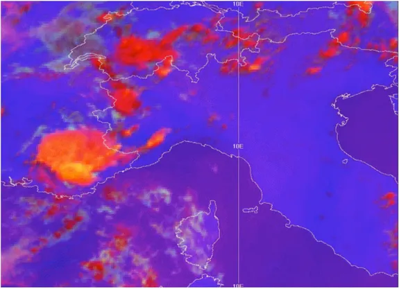
Monitor convective storms, like thunderstorms; they are usually accompanied by strong winds and heavy rainfalls (or hail) and they can create problems to people and properties on Europe and
22
Africa. SEVIRI allows to monitor this kind of weather phenomena from the beginning and to follow it with a continue scan of surface: it is fundamental to issue timely warnings. In the image, convective storms are shown like red areas.
Figure 1.15: satellite’s image of convective storm over Italy and France.
Monitor volcanic ash clouds. This capacity is extremely important to manage air traffics because this kind of clouds are very dangerous for airplane’s engines: when a plane fly thought volcanic ash clouds, ash can enter in airplane’s engines and can stop them. Data about volcanic ash are sent to London and Toulouse VAAC (Volcanic Ash Advisory Centers) which are responsible to warnings advisor for air traffic. New SEVIRI’s algorithms will soon allow to evaluate height, effective radius and others parameter of volcanic ash clouds.
Monitor fog. With the combination of several techniques, Meteosat allows a continuous monitoring of fog’s distribution. This information is still fundamental for air traffic, but for principal road networks and shipping routes too. In the image, the black indicates thick fog; lighter gradients indicate lower intensity of fog. Grey areas are no-fog zones.
23
Figure 1.16: Image of fog over Italy.
As stated previously, SEVIRI scans 12 spectral channels on 3 bands [2] [16] :
CHANNEL
NAME
SPECTRAL BAND CHARACTERISTICS (µM)
Λ
MINΛ
CENΛ
MAX1
VIS0.6
0.56
0.635
0.71
2
VIS0.8
0.74
0.81
0.88
3
NIR1.6
1.50
1.64
1.78
4
IR3.9
3.48
3.90
4.36
5
WV6.2
5.35
6.25
7.15
6
WV7.3
6.85
7.35
7.85
7
IR8.7
8.30
8.70
9.1
8
IR9.7
9.38
9.66
9.94
9
IR10.8
9.80
10.80
11.80
10
IR12.0
11.00
12.00
13.00
11
IR13.4
12.40
13.40
14.40
12
HRV
Wide band (between 0.4 and 1.1 µm)
24
Every channel is accuracy positioned to a specific belt of frequencies; this is because every belt allows to provide information about specific phenomena. Let’s analyze every function’s band.
Wavelengthsof Visible channels are 4, one in high resolution (HRV); they provide information about the quantity of sunlight reflected by Earth and atmosphere. Channels are used to detect clouds, identify their composition and conditions of the surface (snow, water, mountain, flora,….): all this data was used to create images of the planet. These kinds of images are easy to read because human eyes are sensible to the same kind of light (just visible). However, these channels are able to provide data only during the daylight; indeed, during night, these channels are useless. In the images, four visible channels, in order from left to right (channels 1,2,3 and 12); the last image is of the Wide Visible Band:
Figure 1.17: Images of the 4 visible channels of SEVIRI.
Infra-Red channel provide information about radiations issued by Earth; data are available 24/24 hours. With these channels, satellites detect temperature of surface and clouds to estimate, for example, the altitude. Some of these IR bands have the same wavelengths of some important gasses in atmosphere, like ozone and carbon dioxide; so, they are used to pick up information about gasses concentration and clouds’ composition. All the six channels on IR Band is shown, in order from top left to bottom right (channels 4,7,8,9,10 and 11), in images:
25
Figure 1.18: Images of the 6 infra-red channels of SEVIRI.
Water vapor channels are positioned in water vapor’s principal absorption bands. In this band, SEVIRI gives few information about surface but a lot about distribution of water in atmosphere, so, it can determinate the presence of clouds, the index of wetness and the intensity of winds. In images, two WV channels (channels 5 and 6):
Figure 1.19: Images of the 2 water vapor channels of SEVIRI.
With these data, SEVIRI allows to create Earth images from the space with a great resolution.
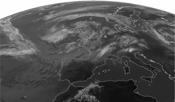
In the Visible band, objects in these images have a color proportional to their reflection capacity: light colors for high reflection capacity, dark color for low reflection capacity; so it is easy to indentify clouds (and storms) and characteristics of surface like desert, mountain, ocean,..
26
Figure 1.20: Clear satellite image of visible band over Europe.
The images in Infra-Red channels instead give information about temperature: dark colors mean cold objects and light colors mean hot objects. So, clouds should be black and the surface should be white; but often, to have a better reading and a better comparing with visible images, IR images are displayed in inverted colors.
27
Sometimes, to mix information from several channels, it is possible to create composed images: Red, Green and Blue (RGB) colors are associated to intensity of three different channels. RGB are usually used to underline particular phenomena. In the image, white are used for clouds (cyan’sgradients for high ice-clouds and red’s gradients for rain-clouds). Surface with flora is green because of high reflection capacity, deserts are ocher and seas are dark because of very low reflection capacity in all channels.
Figure 1.22: RGB image of Europe
1.5.2 Radiometer GERB
GERB [7] (Geostationary Earth Radiation Budget) is a radiometer used to study climate and its evolution; it provides information about radiations on the top of atmosphere within a large IR-band. In this band, the information provided are about clouds and water vapor, forecasting and climate changes. GERB is the first radiometer that gives this kinds of information in a geostationary orbit because previous radiometer was used in LEO. On GEO, it is useful to analyze climatic evolution through clouds and water vapors. Radiometer provides information of full disc Earth every 15 minutes with a spatial sampling of 45x40 km2 at nadir. It has an height of 25 kg and power consumption of
28
detected by a thermo-elastic detector array (Bolometer) of 1x256 pixels, designed to scan full Earth’s disc (18° FOV) in North-South direction:
Figure 1.23: Single strip 1x256 pixels detected by GERB.
Every N_S scan is limited to a strip of 40 ms during MSG rotation so, a full coverage of the disc is provided by a continuously FOV from West to East and back again. The full Earth coverage is complete every 15 minutes.
GERB is composed by two meaning parts: the IOU (Instrument Optical Unit) and the IEU (Instrument Electronic Unit).
IOU is very compact 56x35x33 cm3 and is composed mainly by:
The telescope: a typical astigmatic system with three mirrors;
A de-scanning mirror: it is used to hold the image on the target during the rotation of satellites around its axis. It has a continuously rotation of 50 rpm (rotation per minute), in the opposite direction of satellite, during the scan period of 40 ms;
A wideband detector array. It is a linear thermo-electric array, 1x256 pixels, with its amplifier and processing circuitry, including ASIC and DSP;
A quartz-filter used for change the wavebands (total and short wave) to provide different kind of data;
Calibration block, like SEVIRI. It is composed by a black body on optical path, a solar diffuser to monitor the reflectance of the mirrors, a quartz-filter transmittance and a detector adsorption;
29 A solid-optical-bench structure.
These principal parts of IOU is shown in the image:
Figure 1.24: Main part of IOU in the radiometer GERB.
Instead, the IEU is a small unit, 22x27x25 cm3, used to receive detected data and pass them, in a
specific format, to the spacecraft’s data handling system. Furthermore, IEU gives power to all the instrument’s component.
1.6 Meteosat Third Generation (MTG)
MTG (Meteosat Third Generation) is a new series of satellites that will take place MSG series in a few years. MTG satellites are of 3-tonne class.
30
MTG series is composed by 6 satellites with a lifetime of 8.5 years, first one ready for the launch in 2018; this series guarantee information about meteorological phenomena up to 2030. MTG systems start with cooperation between EUMETSAT and ESA; this one has already contributed to the initial research about technologies of these satellites.
In orbit, the six satellites will be divided in parallel positioned couples: all will be stabilized on 3 axis and their instrument will always point towards Earth; first two satellites will be positioned in geostationary orbit, between 10°E and 10°W above the Equator. The scan of full disc will be available every 10 minutes on 16 several channels, 8 in band of solar spectrum with max resolution of 1 Km and 8 in band of IR spectrum with max resolution of 2 Km. Rapid Scan function will analyze Europe every 2.5 minutes with an additional 0.5 Km max resolution channel in visible band. In details, main instruments on MTG satellites are [9] [10] [19] Errore. L'origine riferimento non è stata trovata.:
Full Disk High Spectral resolution Imagery (FDHSI): Full Disk High Spectral resolution Imagery (FDHSI):
o global scales (Full Disk) over a repeat cycle of 10 minutes;
o 16 channels at spatial resolution of 1 km (8 solar channels, Visible band) and 2 km (8 thermal channels, IR band);
High spatial Resolution Fast Imagery (HRFI):
o local scales (25% of Full Disk, Europe area) over a repeat cycle of 2.5 minutes;
o 4 channels at high spatial resolution: 0.5 km for 2 solar channels (Visible band), 1.0 km for 2 thermal channels (IR band);
Infra-Red Sounding (IRS):
o global scales (Full Disk) over a repeat cycle of 60 minutes;
o spatial resolution of 4 km, providing hyper-spectral soundings at 0.625 cm-1 sampling
in two bands:
Long-Wave-IR (LWIR: 700 – 1210 cm-1 with about 820 spectral samples)
Mid-Wave-IR (MWIR: 1600 – 2175 cm-1 with about 920 spectral samples)
Lightning Imagery (LI):
o global scales (80% of Full Disk) detecting and mapping continuously the optical emission of cloud-to-cloud and cloud-ground discharges;
o Detection Efficiency (DE) between 90% (night) and 40% (overhead sun); UVN Sounding, implemented as GMES Sentinel-4.
This generation of satellites will be divided in 2 principal missions: MTG-I (Imager) and MTG-S (Sounder). Here a timeline of the missions in MTG series:
31
Figure 1.26: Missions of MTG series.
Both of them communicate to the surface with KU-band antenna; KU-band is a belt of microwave
frequencies, from 12 to 18 GHz, used in space communications (it is an international standard).
1.6.1 MTG-S
MTG-S (Meteosat Third Generation – Sounder) mission is composed by 2 geostationary satellites of MTG series with a sounder on board; they are powered by two deployable solar arrays which store energy in some batteries. The sounder is the main innovation of this new program: for the first time, Meteosat satellites will analyze the atmosphere layer-by-layer, just not with only image weather systems, to provide details about chemical composition.
Sounder instrument preliminary parameters are: dimension 1.44x1.30x1.25 km3, mass of about 438 kg and power consumption
of 858 W.
It is composed by more components, most important are shown in the image [16] :
32
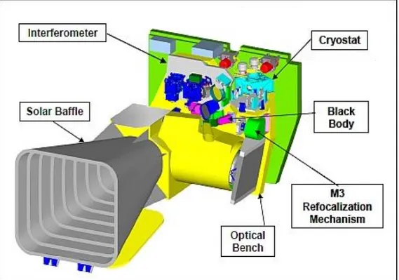
Figure 1.28: Principal parts of the sounder on MTG-S.
Solar baffle deflects the sunlight, the interferometer is on the back side of the sounder to keep images. As SEVIRI, black body and M3 Re-focalization Mechanism are used to take the sounder in initial position. Optical bench is used to adjust lights in optical path; the cryostat is fundamental to hold cold the instrument.
As stated previously, MTG-S will be on board two kinds of interferometers [19] :
The UVN or UVS (Ultraviolet, Visible and Near-infrared Spectrometer); it is a GMES (Global Monitoring for Environment and Security) Sentinel-4, instrument designed for geostationary chemistry applications. It will take measurements in the ultraviolet band (UV: 305 – 400 nm), the visible band (VIS: 400 – 500 nm) and the near infrared band (NIR: 755 – 775 nm) with a spatial resolution of better than 10 km (~8 km). Its observations are restricted to Earth area coverage, from 30° to 65°N in latitude and from 30°W to 45°E in longitude. The observation repeat cycle period will be shorter than or equal to one hour;
The IRS (Infra-Red Sounder) with hyper spectral resolution in thermal spectral domain. For the first time, an instrument will be able to provide information on horizontally, vertically and temporally (4-dimensional) structures of the atmosphere. To provide information about structures of humidity (about 2 km resolution with 10% accuracy) and temperature (about 1 km with 0.5° - 1.5° accuracy), it is required to measure water vapor and carbon monoxide
33
absorption bands with extremely high spectral resolution and accuracy. This is the reason why interferometer is based on an imaging Fourier-interferometer with a hyper-spectral resolution of 0.625 cm-1 wave-number, taking measurements in two bands, the LWIR band (Long-Wave
Infra-Red) and the MWIR band (Mid-Wave Infra-Red) at spatial resolution of 4 Km; the instrument has a global scales over a repeat cycle of 60 minutes.
IRS samples in two bands to provide data about different layer of atmosphere [9]:
Figure 1.29: Spectrum of the wavelengths detected by IRS.
In the image the two bands are shown. In LWIR band (Long-Wave-IR: 700-1210 cm-1), IRS provides
data about ozone (O3) gas, in MWIR band (Mid-Wave-IR: 1600-2175 cm-1), IRS provides data about
34
1.6.2 MTG-I
MTG-I (Meteosat Third Generation – Imager) mission is composed by the other 4 geostationary satellites of MTG program. These kinds of satellites will be similar to MTG-S satellites but they will have on board an imager instead of a sounder. MTG-I mission is planned to add lightning imagers to geostationary satellites to a specifically measure IC (intra-cloud, cloud to cloud) lightning for better locating areas of intensive convection within extended storm systems. In view of a more unified operational GEO observing system, the MTG LI is intended to provide a real time total lightning detection capability of IC and CG (cloud-to-ground) flashes, with no direct discrimination between the two types. Furthermore, MTG-I satellites provide
information for GEOSAR (GEO Search and Rescue) missions and for the DCS (Data Collection System) database [8].
Two principal instruments on board on MTG-I satellites are:
FCI [16] [19] (Flexible Combined Imager), an instrument that will provide information about high-impact weather such as thunderstorms or fog; it will be the follow-on instrument of SEVIRI. Furthermore, will allow to make an important contribution to air-quality monitoring and, with its high-resolution capability in the thermal-infrared, will provide data for fire detection and climate monitoring. This instrument’s mission is divided into another two “easier” missions:
o the FDHSI (Full Disk High-Spectral-resolution Imagery) mission; this instrument uses 16 channels, with a spatial sampling of 1-2 Km on different band, to scan a full disc over a repeat cycle of 10 minutes;
o the HRFI (High spatial Resolution Fast-refresh Imagery) mission; it uses instead 4 channels, with a spatial sampling of 0.5-1.0 km on different band, to scan local area over a repeat cycle of 2.5-5 minutes;
35
Figure 1.31: views of FCI.
Channels of FCI are [15] :
CHANNEL
CENTRE WAVELENGTH
Λ
0(µM)
SPECTRAL WIDTH
ΔΛ
0(µM)
SPATIAL SAMPLING
DISTANCE (DSS)
VIS 0.4 0.444 0.060 1.0 km VIS 0.5 0.510 0.040 1.0 km VIS 0.6 0.640 0.050 1.0 km; 0.5 km* VIS 0.8 0.865 0.040 1.0 km NIR 0.9 0.914 0.020 1.0 km NIR 1.3 1.380 0.030 1.0 km NIR 1.6 1.610 0.050 1.0 km NIR 2.2 2.250 0.050 1.0 km; 0.5 km* IR 3.8 (TIR) 3.800 0.400 2.0 km; 1.0 km* WV 6.3 6.300 1.000 2.0 km WV 7.3 7.350 0.500 2.0 km IR 8.7 (TIR) 8.700 0.400 2.0 km IR 9.7 (O3) 9.660 0.300 2.0 km IR 10.5 (TIR) 10.500 0.700 2.0 km; 1.0 km* IR 12.3 (TIR) 12.300 0.500 2.0 km IR 13.3 (CO2) 13.300 0.600 2.0 kmTable 1.4: 16 channels of FCI. The red channels are used by FDHSI and HRFI. The second value in DSS column (*) is the value of HRFI instruments. TIR as Thermal Infra Red.
36
Figure 1.32: Earth image of every FCI channel.
LI (Lightning Imager), an imaging detection instrument with high resolution. Its most important objective is to add complimentary information to the existing ground lightning detection systems, with the benefit to provide a wider coverage, including poorly populated areas, and a reference to correlate different ground systems and networks. Furthermore, it allows to provide data about atmospheric chemistry and climate monitoring.
37
Chapter 2
Lightning Imager
LI [10] [12] (Lightning Imager) for Meteosat Third Generation is an on board instrument used to provide information to the location and detection of cloud-to-ground and cloud-to-cloud lightning over the full Earth disk from geostationary orbit in day and night conditions. LI’s data from geostationary orbit are regarded as a complementary source of lightning data provided by the ground-based Lightning Location Systems (LLSs); Global LLS networks limit their detection capability mainly on CG flashes. But local LLS
networks are limited on industrialized countries; so lightning data over oceans or Africa are provided with less quality than industrialized countries and data are no homogeneous over all the territory because of network geometry and territorial difference. Instead, LI will provide data over the hemisphere with the same quality: this will be a great vantage because data about climate changes, lightning activities and NOX gas (important for ozone hole and acid rain) will be provided
homogeneously. With this new instrument, in cooperation with the two NOAA GLMs (Geostationary Lightning Mappers on board of GOES-R satellites), the planet will be fully covered [13] .
Primary objectives of LI [24]:
Provide the ability to detect the very first cloud flashes, thus giving valuable additional lead-time for precise warnings of lightning strikes;
Provide lightning data continuously for any location in the FOV (field of view), apply the algorithm and send important information about dangerous storm for the air traffic and people security;
Provide data about convection storms for nowcasting and forecasting;
Improve rainfall measurements when combined with other satellite measurement;
Measure NOX and other gasses to monitor atmospheric chemistry conformation and their effect
on global and local climate changes (effects of these gasses are a matter of great uncertainty at this time, and long-term observations of their sources will prove valuable as the subject develops);
Create a database of lightning events for weather services and security operations
Can be used for validating NWP models (Numerical Weather Prediction is a model used to short-medium weather forecasting; with a lot of weather’s data, powerful computers elaborate nowcasting to make prevision of future possible events);
38
As stated previously, LI must have strict requirements to observe continuously and simultaneously the full visible disk with high temporal resolution.
Requirements necessary to a precision detect IC and CG lightning are provided by ESA; they are [10][11][19]:
PARAMETER
REQUIREMENT
FOV 84% of visible Earth disk (including all Eumetsat member states, instantaneous view) or 16° shifted northward
Spatial sampling < 10 Km at 45° Latitude
Data rate < 30 Mbps
Dynamic range of Earth background (Lbkg) 0 ÷ 296.5 W/(m2 * μm * sr) (night)
Optical pulse dynamic range (LLp) 6.7 ÷ 670 mW/(m² * sr) Sensitivity pulses 4 μJ/(m2 * sr) for 100 km2
Detection Efficiency (DE)
70% as average over the FOV 90% for latitude 45 deg
> 40% over EUMETSAT member states False Alarm Rate 2.5 (false) flashes every second
LI Optical Head Envelope 718 x 1200 x 1456 mm3
Optical pulse spectral range 777.4 ± 0.17 nm with 1.0-1.5 nm spectral pass-band filter Minimum optical pulse duration 0.6 ms
Maximum number of optical pulses (in FOV) 25 in 1 ms 800 in 1 s Background image’s cycle 60 seconds
LI OH overall dimension 715 x 1100 x 1200 mm LI Main Electronics overall dimension 300 x 240 x 160 mm
Table 2.1: Requirements of LI.
LI is composed by one Optical Head (LI OH) and one Electronic control unit (LI Main Electronics); Mass of OH must not exceed 70 kg, 93 kg for OH and Electronic unit, and LI’s max-power consumption is 320 W. OH consists in 4 identical Optical Channel (OC); 4 because all the OH must satisfy technique requirements and every Channel scans a specific cardinal zone. Furthermore, to distinguish true lightning from false one (generated by random noise, sun glints or micro-vibrations),
39
at the same time, on spectral, spatial and temporal domains.
Spectral filtering uses a very narrowband filter centered on the bright lightning O2 triple line
(777.4 nm ± 0.17 nm).
Spatial filtering is achieved with the valuation of lightning’s size: if it is smaller than a typical lightning pulse, it is discarded.
Temporal filtering takes advantage of continues sampling of Earth disk every 1 ms.
A multi-Optical Channel architecture is useful to optimize spectral filtering (narrow band filtering): with a single optical channel, the quantity and the quality of provided data are not sufficient (telescope cannot provide information as required) and the difficulty of on board architecture are considered unacceptable for power consumption, number of operations and elaboration time.
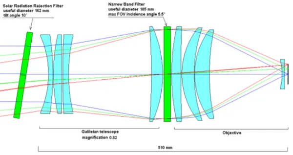
Single optical channel means a very large detector array, about 5 Megapixel, and an high-efficiency electronic system which could have to elaborate about 5 Gigapixel per second in near real time. Furthermore, with a single optical channel, the detector is reduced into a Galileian telescope. In Galileian telescope, an high angle of incidence of blue spectral is not sustained by spectral filter: it will not be uniform.
Figure 2.3: Blue angle of incidence in optical path on Galileian telescope.
In a multi-channel LI, Galileian telescope is no more required. Furthermore, more Optical Channels improves (narrowband) filtering performances.
40 For these reasons, LI has four Optical Channels.
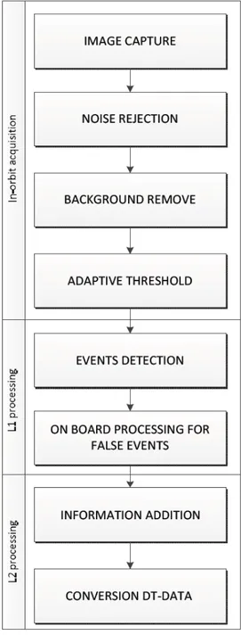
LI has to make more operations to detect flashes; they are divided in 3 principal kinds of processes [10] :
1. In-orbit data acquisition; 2. Level-1 processing; 3. Level-2 processing.
These LI processes are detailed in the following functions, step by step: In- orbit acquisition:
o Earth image acquisition for continuous monitoring of the lightning’s presence in the FOV;
o Calculation of pixel-by-pixel adaptive background to cope with non-uniformities and low terms variations of the image and to reject at the same time noise effects and spurious events;
o Removal of background level from the overall pixel signal to obtain the illumination‘s level of every pixel;
o Use of adaptive thresholds: lower thresholds in low noise dark areas, higher thresholds only for highly illuminated areas;
Level-1 processing:
o Pixels for which the difference between the pixel value and the estimated background signal exceeds the threshold are kept as Detected Transients (DT);
o On-board DTs filtering to reduce number of noise and False Transients (FT)
Level-2 processing
o On-board add information for the ground processing with a dedicated processing electronics (Geolocation, time tagging and radiance-energy association);
o Conversion of the DT video data into digital information (row and column over a digital grid) and conversation in a level compatible with the platform downlink data rate constraints (<30 Mbps).
Main output data of this algorithm are groups of/single lightning events with their location, time and radiance.
41
Figure 2.4: Flux of on-board operation for events detection and data tramission.
2.1 Image capture
As stated previously, Lightning Imager [10] is a single telescope with 4 different channels; they have a focal length of around 600 mm and a pupil size of 110 mm. They use an APS (Active Pixel Sensor) in C-MOS technology with a resolution of 1000x1170 pixels and a time refresh of 1 ms. FOV of this instrument must allow to provide lightning information mainly on Africa (a contribute for global lightning) and on Europe and South-America with lower frequency (ocean too); it is because lightning events are more frequent in the tropical areas like Africa and South-America:
42
Figure 2.5: Annual flash density in MTG FOV.
LI’s FOV is shown in the image:
Figure 2.6: FOV of Lightning Imager.
With a single FOV, LI covers all the zones; but more satellites are necessary to cover a greater part of surface. With the collaboration of USA, more than half of the Earth is covered with high overlap between MTG and GOES-R (East and West GOES-R) FOVs:
43
Figure 2.7: Earth coverage by MTG and GOES-R FOVs.
This kind of FOV has a high distortion: on zenith, the view is perfect (over Equator) but, towards Earth’s edges, the view is highly distorted and, on large nadir angles, pixels are quiet indistinguishable: this is a big problem because pixels indistinguishable means indistinguishable events [10] :
Figure 2.8: Deformations of detected images.
Because of this problem, LI must have some specific algorithms and instruments to correct this problem.
44
2.2 Noise rejection
Principal problems of image capture is the noise: an high level of noise make unreadable the image provided by the telescope. In the following image, different FER (False Event Rate) are shown for the same scanned zone: in a time of 500 ms, a FER of 40000 (so 20000 false events in 500 ms) does not allow to provide accuracy data and some filter are necessary to detect true events. With a FER of 400000 the image is completely unreadable [11] .
Figure 2.9: Examples of False Error Rate over Europe.
There are two kinds of noise: internal noise and external noise. Internal noise is generated by the component in the satellite’s instruments like telescope and electronic components. On the other hand, external noise is due to external conditions of atmosphere and light.
Main causes of internal noise are [15] :
Electronic noise: this is a noise typical of electronic components on board, specially from power source and amplifier stages.
Thermo-mechanical noise: this noise comes from movement and rotation of mechanical mobile part and from thermal source in telescope.
45
Stray light noise: this noise is made by lights which do not follow the correct path and, for this reason, creates interference with useless light.
On the other hand, the main causes of external noise are:
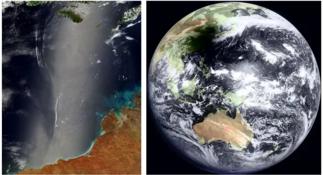
Cloud radiation: a part of solar radiation is reflected by clouds. In images, this radiation is interpreted as light and it can be added to the Detected Events (DE).
Sun glint and solar eclipse: sun glint is an optical phenomenon where the sun light is reflected by oceans with the same angle of satellite’s view. Sun glint and solar eclipse are considered noise because both of them change the radiance level of an area: high level of radiance can be exchanged to lightning events.
Figure 2.10: Examples of sun glint and solar eclipse detected by satellite.
Particles flux: especially in Van Allen belt, it can modify the IFOV with the reflection of sunlight in several bands or with a magnetic contribute which deflect light.
Jitter: it is a typical video phenomenal which occurs when the horizontal lines of two consecutive frames are not synchronized because of movement or micro-vibrations. This noise is particularly problematic in time subtracting of two frame to identify a lightning events: a jitter can create a False Detect [11] .
46
Figure 2.11: Jitter example by frame subtraction.
2.3 Background removal and adaptive threshold
Background is defined as all image’s object considered static in a short time frame. The contrast between background and lightning radiance determinate the capability of detect event: this contrast set SNR (Signal to Noise Ratio) level to detect lightning events. When SNR is high, for example during the night, dark background allows to detect lightning events and clouds.
47
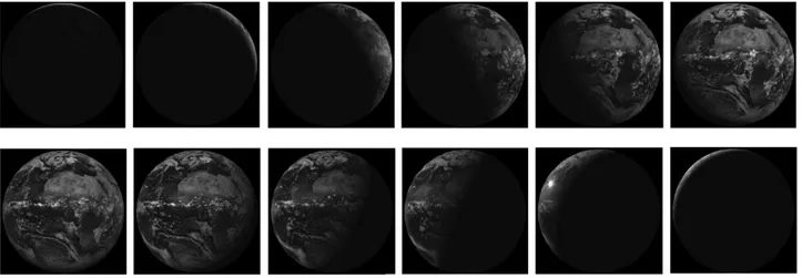
But, for a better readability, background removal is not sufficient. SNR value is also imposed by light condition like day and night or solar eclipse. It is clear in the image: every two hours, the in-orbit view changes and it is not easy to provide any data or image.
Figure 2.13: Surface bright condition every 2 hours.
During the night, low level of light cannot allow to distinguish anything on the ground. In these critical cases is necessary an adaptive threshold to detect lightning events and provide every kind of information [14] .
Figure 2.14: Background trend in a day. Red spikes are lightning events.
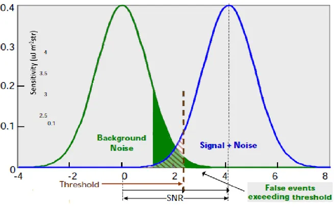
An adaptive threshold is the best solution of background in-homogeneity. In fact, with just a single low threshold level, there could be a large numbers of lightning and false events and, with a single high threshold level, there could be a few lightning events and some others, with low radiance level, could
48
be discarded. Threshold must not be too high because a lot of lightning events could not be detected [9]. In Figure 2.15, it is possible to see what happen with high threshold: some events is not detected because their radiance level is lower than threshold level.
Figure 2.15: Distributions of background and Background + signal in SNR scale. Also threshold used to optimize SNR value.
For this reason, a trade-off between detection sensitivity and false event rates are necessary.
All problems are summarizedin the Figure 2.16. In the daylight, a high level of background radiance fixes a high value of threshold to detect lightning events. But only a single level of threshold is not sufficient because of the light during the day is not homogeneous. So, in the daylight, there are more than one threshold (Threshold 1 and Threshold 2); in some cases, lightning on top of bright background is not recognized by its bright radiance but by its transient short pulse character: in these cases a temporal filtering is used. A critical time is on sunset because radiance level of background decrees rapidly and events are hardly detectable: during sunset, threshold must change quickly. During the night instead, just one threshold is necessary to detect lightning events. [14]
49
Figure 2.16 : adaptive thresholds.
This specific criteria is not easy to apply because background removal and adaptive threshold are different for every pixels or zones in the images. As shown in previously images, on sunset, a part of surface is in daylight but a part is dark because of night and the LI must differentiate the two zones to subtract different background and apply a different level of threshold.
All these operations allow to detect “easily” an event.
2.4 Events detection and on-board processing for FEs
Without the previous operations, the events detection is quite impossible. This image shows a single lightning event detected over Ethiopia: without a deep zoom is impossible to distinguish the event [10].
50
For this reason, every LI’s image goes through the algorithm of detection for background removal and adaptive threshold. In this phase, filtering is carried out. There are 3 kinds of filter:
Spatial filter: compare the radiation of detected event in IFOV (Instant FOV) with the typical lightning event radiation’s view;
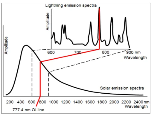
Spectral filter: a special narrow band filter centered on a wavelength of 777,4 nm make a frequency filtering. 777,4 nm is the wavelength of the first ionized energy of Oxygen:
Figure 2.18: Wavelength of first ionized energy of Oxygen
Temporal filter: temporal filtering is simply a time compare between pulse and background which is considered constant in the time scale of seconds.
If these 3 filtering are not sufficient, a frame-to-frame background subtracting is used. This is a technique used when the radiance ratio between lightning and background is still under the threshold. With these 3 levels of filtering, almost all the false events are eliminated. False events are not related to a real lightning but are due to noise or distortions or artificial light on the surface: they must be eliminated for a correct now/forecasting and data providing. Figure 2.19 shows the difference between filtered and not-filtered scans [15] :
51
Figure 2.19: Difference between no-filtered and filtered scans.
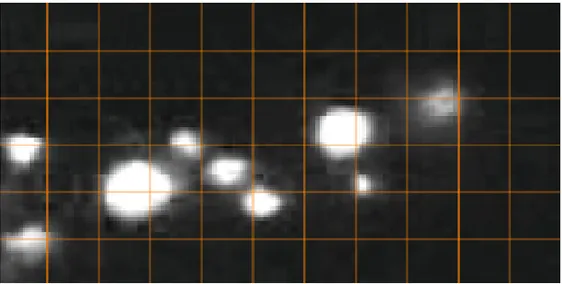
Obviously, this optimal condition of lightning detection is possible only if all the previous technique were used. Images after background removal, adaptive threshold, filtering and event detection is similar to this one:
Figure 2.20: Events detected after background remove, adaptive threshold and filtering.
Now, events are more definite and, with a grid in background, it is possible to detect the location and the size of lightning.