2021-01-21T09:32:03Z
Acceptance in OA@INAF
The ASKAP EMU Early Science Project: radio continuum survey of the Small
Magellanic Cloud
Title
þÿJoseph, T. D.; Filipovi, M. D.; Crawford, E. J.; Bojii, I.; Alexander, E. L.; et al.
Authors
10.1093/mnras/stz2650
DOI
http://hdl.handle.net/20.500.12386/29901
Handle
MONTHLY NOTICES OF THE ROYAL ASTRONOMICAL SOCIETY
Journal
490
Number
T. D. Joseph,
1?
M. D. Filipovi´
c,
2
E. J. Crawford,
2
I. Bojiˇ
ci´
c,
2
E. L. Alexander,
1
G. F. Wong,
2,3
H. Andernach,
4
H. Leverenz,
2
R. P. Norris,
2,3
R. Z. E. Alsaberi,
2
C. Anderson,
3
L. A. Barnes,
2
L. M. Bozzetto,
2
F. Bufano,
6
J. D. Bunton,
5
F. Cavallaro,
6
J. D. Collier,
2,7
H. D´
enes,
8
Y. Fukui,
9,10
T. Galvin,
2,3
F. Haberl,
11
A. Ingallinera,
6
A. D. Kapinska,
12
B. S. Koribalski,
3
R. Kothes,
13
D. Li,
14,15
P. Maggi,
16
C. Maitra,
11
P. Manojlovi´
c,
2,3
J. Marvil,
12
N. I. Maxted,
2,17
A. N. O’Brien,
2,3
J. M. Oliveira,
18
C. M. Pennock,
18
S. Riggi,
6
G. Rowell,
19
L. Rudnick,
20
H. Sano,
9,10
M. Sasaki,
21
N. Seymour,
22
R. Soria,
15,23
M. Stupar,
2
N. F. H. Tothill,
2
C. Trigilio,
6
K. Tsuge,
10
G. Umana,
6
D. Uroˇsevi´
c,
24,25
J. Th. van Loon,
18
E. Vardoulaki,
26
V. Velovi´
c,
2
M. Yew,
2
D. Leahy,
27
Y.-H. Chu,
28
M. J. Micha lowski,
29
P. J. Kavanagh,
30
K. R. Grieve
2
1Department of Physics and Astronomy, University of Manchester, Oxford Road, Manchester, M13 9PL, UK 2Western Sydney University, Locked Bag 1797, Penrith South DC, NSW 2751, Australia
3CSIRO Astronomy and Space Science, PO Box 76, Epping, NSW 1710, Australia
4Depto. de Astronom´ıa, DCNE, Universidad de Guanajuato, Apdo. Postal 144, Guanajuato, CP 36000, Gto., Mexico 5School of Physics, The University of New South Wales, Sydney, 2052, Australia
6INAF Osservatorio Astrofisico di Catania, via Santa Sofia 78, I-95123 Catania
7The Inter-University Institute for Data Intensive Astronomy (IDIA), Department of Astronomy, University of Cape Town, Rondebosch, 7701, South Africa
8ASTRON - Netherlands Institute for Radio Astronomy, 7991 PD, Dwingeloo, The Netherlands 9Institute for Advanced Research, Nagoya University, Furo-cho, Chikusa-ku, Nagoya 464-8601, Japan 10Department of Physics, Nagoya University, Furo-cho, Chikusa-ku, Nagoya 464-8601, Japan 11Max-Planck-Institut f¨ur extraterrestrische Physik, Giessenbachstraße, D-85748 Garching, Germany 12National Radio Astronomy Observatory, 1003 Lopezville Rd., Socorro, NM 87801, USA
13Dominion Radio Astrophysical Observatory, Herzberg Programs in Astronomy and Astrophysics, National Research Council Canada, PO Box 248, Penticton, BC V2A 6J9, Canada
14CAS Key Laboratory of FAST, National Astronomical Observatories, Chinese Academy of Sciences, Beijing, 100101, China 15School of Astronomy and Space Sciences, University of Chinese Academy of Sciences, Beijing 100049, China
16Observatoire Astronomique de Strasbourg, Universit´e de Strasbourg, CNRS, 11 rue de l’Universit´e, F-67000 Strasbourg, France 17School of Science, The University of New South Wales, Australian Defence Force Academy, Canberra, 2600, Australia 18Lennard-Jones Laboratories, Keele University, ST5 5BG, UK
19School of Physical Sciences, The University of Adelaide, Adelaide 5005, Australia
20School of Physics and Astronomy, University of Minnesota, Minneapolis, MN 55455, USA
21Remeis Observatory and ECAP, Universit¨at Erlangen-N¨urnberg, Sternwartstr. 7, D-96049 Bamberg, Germany 22International Centre for Radio Astronomy Research, Curtin University, Bentley, WA 6102, Australia
23Sydney Institute for Astronomy, School of Physics A28, The University of Sydney, Sydney, NSW 2006, Australia 24Department of Astronomy, Faculty of Mathematics, University of Belgrade, Studentski trg 16, 11000 Belgrade, Serbia 25Isaac Newton Institute of Chile, Yugoslavia Branch
26Argelander-Institut f¨ur Astronomie, Auf dem H¨ugel 71, D-53121 Bonn, Germany
27Department of Physics and Astronomy, University of Calgary, University of Calgary, Calgary, Alberta, T2N 1N4, Canada 28Institute of Astronomy and Astrophysics, Academia Sinica (ASIAA), Taipei 10617, Taiwan
29Astronomical Observatory Institute, Faculty of Physics, Adam Mickiewicz University, ul. S loneczna 36, PL-60-286 Pozna´n, Poland 30School of Cosmic Physics, Dublin Institute for Advanced Studies, 31 Fitzwillam Place, Dublin 2, Ireland
Accepted XXX. Received YYY; in original form ZZZ
ABSTRACT
We present two new radio continuum images from the Australian Square Kilometre Ar-ray Pathfinder (ASKAP) survey in the direction of the Small Magellanic Cloud (SMC). These images are part of the Evolutionary Map of the Universe (EMU) Early Sci-ence Project (ESP) survey of the Small and Large Magellanic Clouds. The two new source lists produced from these images contain radio continuum sources observed at 960 MHz (4489 sources) and 1320 MHz (5954 sources) with a bandwidth of 192 MHz and beam sizes of 30.000×30.000 and 16.300×15.100, respectively. The median Root
Mean Squared (RMS) noise values are 186 µJy beam−1 (960 MHz) and 165 µJy beam−1
(1320 MHz). To create point source catalogues, we use these two source lists, together with the previously published Molonglo Observatory Synthesis Telescope (MOST) and the Australia Telescope Compact Array (ATCA) point source catalogues to estimate spectral indices for the whole population of radio point sources found in the survey region. Combining our ASKAP catalogues with these radio continuum surveys, we found 7736 point-like sources in common over an area of 30 deg2. In addition, we
re-port the detection of two new, low surface brightness supernova remnant candidates in the SMC. The high sensitivity of the new ASKAP ESP survey also enabled us to detect the bright end of the SMC planetary nebula sample, with 22 out of 102 opti-cally known planetary nebulae showing point-like radio continuum emission. Lastly, we present several morphologically interesting background radio galaxies.
Key words: Magellanic Clouds – radio continuum – catalogues – SNRs – YSO – AGNs – PNe
1 INTRODUCTION
This is an exciting time for the study of nearby galaxies. These nearby external galaxies offer an ideal laboratory, since they are close enough to be resolved, yet located at relatively well known distances (see e.g. Pietrzy´nski et al. 2019). New generations of Magellanic Cloud (MC) surveys across the entire electromagnetic spectrum reflect a major opportunity to study different objects and processes in the elemental enrichment of the Interstellar Medium (ISM). The study of these interactions in different domains, including radio, optical and X-ray, allow a better understanding of objects such as supernova remnants (SNRs), planetary neb-ulae (PNe), (Super)Bubbles and their environments, young stellar objects (YSOs), symbiotic (accreting compact object) binaries and Wolf-Rayet (WR) wind-wind-collision binaries. Various new high resolution (∼100) and high sensitivity surveys of the Small and Large Magellanic Clouds (MCs), such as XMM–Newton and Chandra (X-rays; see e.g. Haberl et al. 2012b), Herschel (Gordon et al. 2011) and Spitzer (IR; Meixner et al. 2006), UM/CTIO Magellanic Cloud Emis-sion Line Survey (MCELS, optical; Winkler et al. 2005) and ATCA/MOST (radio), provide a solid base for detailed multi-wavelength studies of radio objects within and behind the MCs.
Our main area of interest is the radio objects natal to the MCs, particularly SNRs and PNe. To date, some 85 SNRs in the MCs have been identified, with a further 20 can-didates awaiting confirmation (Maggi et al. 2016; Bozzetto et al. 2017). Similarly, over 50 PNe (Filipovi´c et al. 2009; Bo-jiˇci´c et al. 2010; Leverenz et al. 2016, 2017) and hundreds of H ii regions and YSOs have been identified (see for example Oliveira et al. 2013). Over 8500 radio sources have also been
? E-mail: [email protected] (TDJ)
detected in the region of the Clouds – mainly AGN, radio galaxies and quasars (Wong et al. 2012b; Collier 2016, Grieve et al. in prep.). Additionally, some comprehensive studies of the magnetic fields of the MCs have been undertaken with the present generation of radio continuum surveys (ATCA; Gaensler et al. 2005; Mao et al. 2008, 2012).
In this paper, we focus on the Small Magellanic Cloud (SMC), a dwarf irregular galaxy. Its proximity (∼60 kpc; Hilditch et al. 2005) enables us to conduct detailed radio frequency studies of its gas and stellar content, without the complication of the foreground emission and absorption we encounter when working within our own Galaxy. For these reasons, the SMC has been the subject of many radio studies over several decades.
Starting in the mid 1970s, the SMC has been the sub-ject of both single dish and interferometric radio continuum surveys. These monitoring campaigns have produced over a dozen catalogues of sources towards the SMC (Clarke 1976; McGee et al. 1976; Haynes et al. 1986; Wright & Otrupcek 1990; Filipovi´c et al. 1997; Turtle et al. 1998; Filipovi´c et al. 1998; Filipovi´c et al. 1997, 2002; Payne et al. 2004; Filipovi´c et al. 2005; Reid et al. 2006; Payne et al. 2007; Wong et al. 2011a; Crawford et al. 2011; Wong et al. 2011b, 2012a,b; For et al. 2018) (see also Table 1 in Wong et al. 2011b, for details).
For the reasons mentioned above, the SMC was also selected as a prime target for the Early Science Project (ESP) of the newly built Australian Square Kilometre Ar-ray Pathfinder (ASKAP; Johnston et al. 2008). ASKAP is a radio interferometer that allows us to survey the SMC with regularly sampled observations. ASKAP also provides sensi-tivity down to theµJy range as well as a large field of view of 30 deg2 (Murphy et al. 2013). The goal of this project is to produce high sensitivity and high resolution continuum images of the MCs as well as to catalogue discrete radio continuum sources.
an RMS noise level of<30 µJy, requiring 380 hours of obser-vation time. This survey uncovered over 3000 distinct radio sources out to a redshift of 2. ASKAP’s higher resolution and increased sensitivity will be able to achieve such results on a much shorter time scale (see Fig. 1 in Franzen et al. 2015).
Another obvious advantage of ASKAP is the size of the field of view. For example, the Sydney University Molonglo Sky Survey (SUMSS) would need ∼16 fields and ∼192 hours to cover the ASKAP EMU SMC survey area to the required sensitivity (see Mauch et al. 2003); in contrast the ASKAP observations were composed of eight fields of about 12 hours each (a total of 96 hours).
In this paper we present two new catalogues from the ASKAP ESP surveys for different types of radio continuum sources towards the SMC. These catalogues were obtained from images taken at 960 MHz (λ = 32 cm) and 1320 MHz (λ = 23 cm). For the point source catalogue, we combine the ASKAP data with the previously published MOST cata-logue (Turtle et al. 1998; Wong et al. 2011b) and the ATCA λ= 20, 13, 6 and 3 cm catalogues (Wong et al. 2011b, 2012a, and references therein).
The paper is laid out as follows: Section 2 describes the data used to create the source lists. In section 3.1 we describe the source detection methods used, section 3.2 describes the new ASKAP source catalogues and in section 3.3 we com-pare our work to previous catalogues of point sources to-wards the SMC. Sections 4 and 5 describe the latest ASKAP SMC populations of SNRs and PNe, respectively. In Sec-tion 6, we briefly discuss other sources of interest, including those behind the SMC.
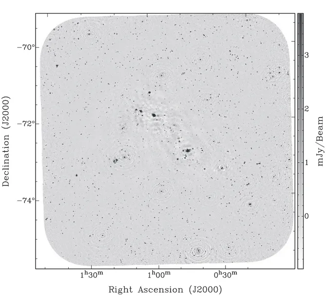
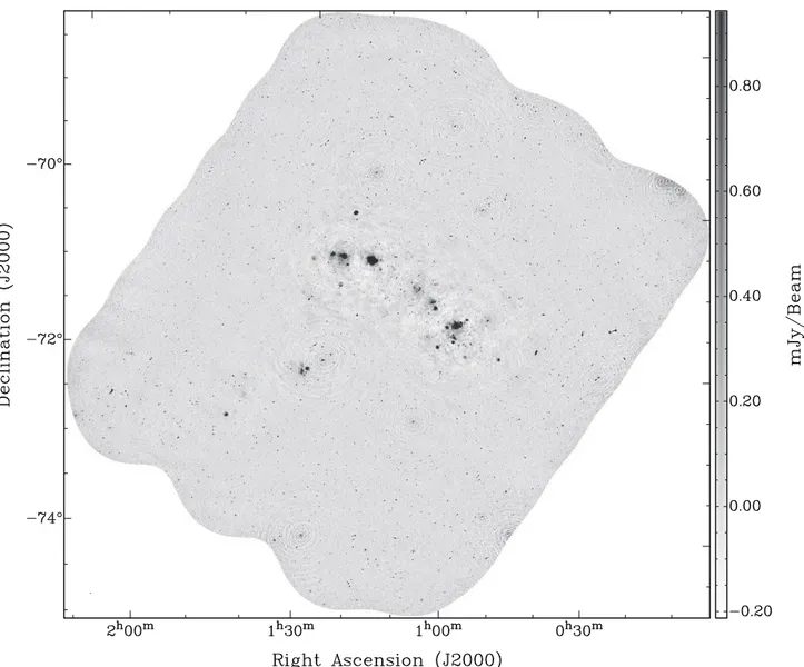
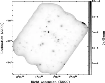
2 DATA, OBSERVING AND PROCESSING The SMC was observed as part of the ASKAP commission-ing and early science verification (DeBoer et al. 2009; Hotan et al. 2014; McConnell et al. 2016). Here, we present obser-vations at 960 MHz taken on 2017 September 3 (Figure 1; using 12 antennas: 2, 3, 4, 6, 12, 14, 16, 17, 19, 27, 28, and 30), and at 1320 MHz on 2017 November 3 - 5 (Figure 2, using 16 antennas: 1, 2, 3, 4, 5, 6, 10, 12, 14, 16, 17, 19, 24, 27, 28, 30). The H i spectral and dynamical analyses of the 1320 MHz data have been presented in McClure-Griffiths et al. (2018) and Di Teodoro et al. (2019) respectively.
We note that the current observations were made with only 33 per cent and 44 per cent (for 960 MHz and 1320 MHz respectively) of the full ASKAP antenna configuration and 66 per cent of the final bandwidth that will be available in the final array. We believe that with the full array, we will be able to achieve a factor of two increase in sensitivity compared to what is currently possible.
A bandwidth of 192 MHz was used and the maximum baseline for these observations was 2.3 km. The observations cover a total field of view of 30 deg2, with exposure times of 10 to 11 hours per pointing. To optimise sensitivity and
2011). For both sets of images we processed the data with the multiscale clean algorithm, noting from our previous work (Wong et al. 2011a) that the largest detectable features were ∼19200. Therefore, we selected spacial scales of 19200, 9600and 4800 as a geometric progression. We also noted features on the scale of 1600, and so this spatial scale was also selected. The 1320 MHz image was cleaned and then mosaiced. For the 960 MHz image, we set the pixel size to 600, and set the restoring beam to 3000× 3000in order to maximise our reso-lution and sensitivity and to more easily compare these new results with other SMC surveys referenced in this work.
The properties of the 960 MHz and 1320 MHz images are summarised in Table 1. These two new ASKAP images are shown in Figures 1 and 2, with zoomed in views showing the resolved structure of the emission in Figures. 3 and 4. Figures 5 and 6 show the RMS maps generated by the source finding software, aegean (Hancock et al. 2012, 2018) for the 960 MHz and 1320 MHz images respectively.
We note that our ESP 960 MHz image was made at very early stages of the ASKAP testing and a range of is-sues, such as positional accuracy and calibration, were dis-covered. We have made every effort to identify and correct these problems. The 1320 MHz image as made at a later date when these issues were already known and could therefore be avoided, mitigated or corrected as needed.
3 ASKAP ESP SMC SOURCE CATALOGUES 3.1 Source detection
The aegean source finding software was used to create an overall catalogue of sources from the ASKAP images. Due to the combination of the multiple beams and arte-facts from bright sources, images from ASKAP have variable noise across the field. This variable noise must be parame-terised before source-finding to ensure that accurate source thresholds are determined. To do this, noise (RMS) and background level maps were made using the BANE routine in aegean, with its default parameters. BANE uses a grid al-gorithm with a sliding box-car and sigma-clipping approach, with the resulting maps being at the same pixel scale as the input images (for further detail, see Hancock et al. 2018). The maps were then used with the default parameters in aegean to create the initial source lists at 5σ level. Visual inspection of the sources was carried out to verify detections from the initial source lists.
3.2 Source Catalogues
In total, we found 4489 and 5954 point sources in our new ASKAP 960 MHz and 1320 MHz images, respectively (see Tables 2 and 3). There are 3536 unique sources that have both ASKAP 960 MHz and 1320 MHz flux densities. This catalogue excludes known SMC SNRs, PNe and H ii regions which are listed separately (see Sections 4 and 5).
Table 1. Properties of the 960 MHz and 1320 MHz radio continuum images as well other MOST/ATCA surveys used in this study.
ν λ Telescope Median RMS Best RMS Beam Size Total number Reference
(MHz) (cm) (µJy beam−1) (µJy beam−1) (arcsec) of point sources
1320 23 ASKAP 165 55 16.3 × 15.1 5954 This work
960 32 ASKAP 186 110 30.0 × 30.0 4489 This work
843 36 MOST 700 500 40.0 × 40.0 1689 Wong et al. (2011b)
1400 20 ATCA 700 600 17.8 × 12.2 1560 Wong et al. (2011b)
2370 13 ATCA 400 300 45.0 × 45.0 742 Wong et al. (2011b)
4800 6 ATCA 700 500 30.0 × 30.0 601 Wong et al. (2012a)
8640 3 ATCA 800 700 20.0 × 20.0 457 Wong et al. (2012a)
Figure 1. ASKAP ESP image of the SMC at 960 MHz. The beam size is 30.000× 30.000and the side scale bar represents the image grey scale intensity range.
Figure 2. ASKAP ESP image of the SMC at 1320 MHz. The beam size is 16.300× 15.100and the side scale bar represents the image grey scale intensity range.
We combine our two new ASKAP catalogues of point sources with previously published source lists from MOST (at 843 MHz) and ATCA (1400, 2370, 4800 and 8640 MHz). To do this, we used a 1000 search radius to find common sources and found a total of 7736 discrete sources which we list in Table 4. Out of these 7736 sources, there are 659 sources that do not have any ASKAP flux densities and 112 that do not have MOST/SUMSS flux densities.
Where possible, we also list the estimated spectral in-dex (α)1 of the source including error (Table 4; Col. 12). We
also note that there are 49 (∼0.5 per cent of the total pop-ulation) sources in Table 4 with questionableα estimates of α < −4 and α > +2.5. Where the α values are extreme we flag those sources to emphasis caution. The reasons behind
1 Defined as S
ν ∝να, where: Sν is flux density,ν is frequency, andα is spectral index.
such unrealisticα for these few sources (<0.3 per cent out of our 7736 sources) are twofold. One is that the flux density measurements are made between only two nearby frequency bands (such as for example 1400/1320 MHz or 960/843 MHz) where a small change (or error) in size or flux density leads to large changes and unrealistic estimates inα. The second issue is that almost all of such sources lie near near the edges of the field where uv coverage and sensitivity are significantly poorer.
Non-point sources, such as blended and extended sources, were flagged and excised to leave only a catalogue of point sources. Although not used in the further analysis, we provide estimates of positions and flux densities for detected non-point sources. We present the results from both cata-logues in Tables 5 and 6 where a total of 282 and 641 non-point sources are found at 960 MHz and 1320 MHz surveys, respectively. Because of the different resolution across the various SMC surveys, some of these listed non-point sources
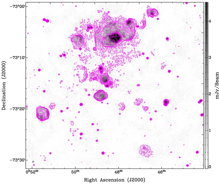
Figure 3. ASKAP ESP image of the SMC N 19 region at 1320 MHz (grey scale and contours). Magenta contours are: 0.3, 0.5, 0.7, 1, 1.5, 2, 3, 5, 7, 10 and 15 mJy beam−1. The beam size of 16.300× 15.100is shown as a small black ellipse in the lower left corner.
Table 2. Point source catalogue derived from our ASKAP 960 MHz image. The catalogue at 960 MHz consists of 4489 point sources. The full table is available in the online version of the article.
Source Name RA (J2000) Dec (J2000) S960MHz
No. ASKAP hh mm ss ◦ 0 00 (mJy)
1 J000437–744211 00:04:36.52 –74:42:11.0 4.0±0.5 2 J000506–751559 00:05:05.77 –75:15:58.6 4.0±0.5 3 J000508–745454 00:05:07.97 –74:54:53.6 16.0±0.5 4 J000545–741232 00:05:44.94 –74:12:31.6 16.9±0.6 5 J000550–744806 00:05:49.77 –74:48:05.9 27.7±0.5 6 J000550–742134 00:05:50.46 –74:21:34.4 3.6±0.5 7 J000603–743754 00:06:03.48 –74:37:54.1 10.9±0.5 8 J000608–740148 00:06:08.34 –74:01:47.6 8.2±0.6 9 J000608–740240 00:06:08.50 –74:02:40.2 9.4±0.6 10 J000609–740538 00:06:09.42 –74:05:38.3 2.9±0.6
could be resolved in one survey but could appear as a point
Table 3. Point source catalogue derived from our ASKAP 1320 MHz image. The catalogue at 1320 MHz consists of 5954 point sources. The full table is available in the online version of the article.
Source Name RA (J2000) Dec (J2000) S1320MHz
No. ASKAP hh mm ss ◦ 0 00 (mJy)
1 J000537–715839 00:05:36.81 –71:58:39.2 5.3±0.9 2 J000547–722502 00:05:46.55 –72:25:01.9 3.8±0.5 3 J000646–720801 00:06:45.91 –72:08:01.2 2.1±0.3 4 J000648–722252 00:06:48.25 –72:22:51.8 10.1±0.3 5 J000653–715740 00:06:52.59 –71:57:40.2 36.3±0.4 6 J000654–722034 00:06:54.07 –72:20:34.2 2.1±0.4 7 J000713–714611 00:07:12.94 –71:46:10.6 4.1±0.6 8 J000726–720631 00:07:26.15 –72:06:30.8 3.4±0.2 9 J000732–720732 00:07:31.97 –72:07:32.2 1.4±0.2 10 J000739–721026 00:07:38.64 –72:10:26.1 2.1±0.4
source in another and as such they would not be listed in Tables 5 or 6.
Figure 4. ASKAP ESP image of the SMC N 66 and SNR 1E0102-72 region at 1320 MHz (grey scale and contours). Magenta contours are: 0.3, 0.5, 0.7, 1, 1.5, 2, 3, 5, 7, 10 and 15 mJy beam−1. The beam size of 16.300× 15.100is shown as a small black ellipse in the lower left corner.
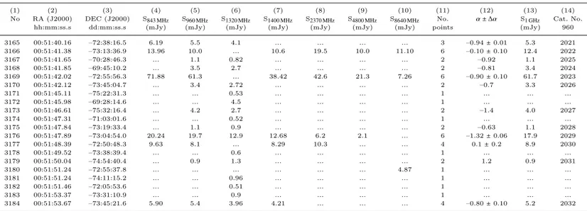
Table 4. An excerpt from the combined catalogue of point sources. These sources should be referred to as EMU-ESP-SMC-ffff NNNN. The full table is available in the online version of the article
.
(1) (2) (3) (4) (5) (6) (7) (8) (9) (10) (11) (12) (13) (14) (15)
No RA (J2000) DEC (J2000) S843 MHz S960 MHz S1320 MHz S1400 MHz S2370 MHz S4800 MHz S8640 MHz No. α ± ∆α S1 GHz Cat. No. Cat. No.
hh:mm:ss.s dd:mm:ss.s (mJy) (mJy) (mJy) (mJy) (mJy) (mJy) (mJy) points (mJy) 960 1320
3165 00:51:40.16 –72:38:16.5 6.19 5.5 4.1 ... ... ... ... 3 –0.94±0.01 5.3 2021 2276 3166 00:51:41.38 –73:13:36.9 13.96 10.0 ... 10.6 19.5 10.0 11.10 6 –0.10±0.10 12.4 2022 ... 3167 00:51:41.65 –70:28:46.3 ... 1.1 0.82 ... ... ... ... 2 –0.92 1.1 2025 2278 3168 00:51:41.85 –69:45:10.2 ... 3.5 2.7 ... ... ... ... 2 –0.81 3.4 2024 2279 3169 00:51:42.02 –72:55:56.3 71.88 61.3 ... 38.42 42.6 21.3 7.26 6 –0.90±0.10 61.7 2023 ... 3170 00:51:42.12 –73:45:04.7 ... 3.4 2.72 ... ... ... ... 2 –0.7 3.3 2026 2280 3171 00:51:45.11 –75:22:31.3 ... ... 0.53 ... ... ... ... 1 ... ... ... 2281 3172 00:51:45.98 –69:28:14.6 ... ... 4.5 ... ... ... ... 1 ... ... ... 2282 3173 00:51:46.61 –75:32:16.4 ... 4.2 2.7 ... ... ... ... 2 –1.4 4.0 2027 2283 3174 00:51:47.31 –71:03:01.6 ... ... 0.52 ... ... ... ... 1 ... ... ... 2284 3175 00:51:47.84 –73:19:33.4 ... 1.1 0.9 ... ... ... ... 2 –0.63 1.1 2028 2285 3176 00:51:47.89 –73:04:54.0 20.24 19.7 12.9 12.68 6.2 2.1 ... 6 –1.32±0.06 17.9 2029 2286 3177 00:51:48.39 –72:50:48.3 9.63 8.1 ... 8.29 10.3 ... ... 4 0.1±0.2 8.9 2030 ... 3178 00:51:49.52 –73:38:39.4 ... ... 0.6 ... ... ... ... 1 ... ... ... 2287 3179 00:51:50.04 –74:54:40.4 ... 0.9 1.3 ... ... ... ... 2 1.2 0.9 2031 2288 3180 00:51:51.24 –72:55:37.8 ... ... ... ... ... ... 4.87 1 ... ... ... ... 3181 00:51:51.24 –74:11:15.2 ... ... 0.96 ... ... ... ... 1 ... ... ... 2289 3182 00:51:51.46 –72:05:53.6 ... ... 0.51 ... ... ... ... 1 ... ... ... 2290 3183 00:51:53.37 –73:31:10.9 ... ... 0.9 ... ... ... ... 1 ... ... ... 2291 3184 00:51:53.67 –73:45:21.6 5.90 5.4 3.96 4.21 ... ... ... 4 –0.80±0.10 5.2 2032 2292
3.3 Comparison with previous catalogues
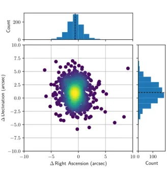
We compare position differences (∆RA and ∆DEC) between our new ASKAP images and previous catalogues at 843 MHz (see Figure 7) and 1400 MHz (see Figure 8). We did not find any significant shift in position in our 1320 MHz vs. 1400 MHz position comparison. For the 889 sources in com-mon, we found that the ∆RA=−0.5800 (SD=1.5000) and ∆DEC=+1.0300 (SD=1.9500). Somewhat worse results are
reported for the 843 MHz vs. 960 MHz comparison of 1509 sources with ∆RA=+2.9000(SD=2.6500) and ∆DEC=−1.4500 (SD=2.9200). These position differences are only a small frac-tion of the beamsize at the given frequency.
Positional shifts of ∼300 in our 960 MHz image are not insignificant, especially if we want to look for multiband counterparts. The reason for the discrepancy lies in the fact that this image comes from the ASKAP testing and early operation period where a number of issues were found and
Figure 5. RMS map of the 960 MHz ASKAP observations, pro-duced by BANE with the default parameters. The image is of the same pixel scale as in Figure 1. Higher RMS levels are found at the edge of the field (where only one beam is present) and around the brighter sources.
Figure 6. RMS map of the 1320 MHz ASKAP observations, pro-duced by BANE with the default parameters. The image is of the same pixel scale as in Figure 2. Higher RMS levels are found at the edge of the field (where only one beam is present) and around the brighter sources.
acknowledged. Specifically, throughout the paper we use the coordinates from other SMC surveys for the various sources wherever possible. An excerpt of the combined point source catalogue is shown in Table 4.
In order to assess the reliability of our integrated flux values, we compared the values on compact (extended H ii regions are excluded) sources to catalogue values from other nearby frequencies. We performed two sets of comparisons: our ASKAP 960 MHz values with the values from MOST at 843 MHz and our ASKAP 1320 MHz values with the ATCA 1400 MHz values. The agreement is excellent, as can be seen in Figures 9 and 10.
As a quick check on flux density scales, we fit SASKAP=
k ×Sother+ z, allowing for some small zero level offsets (z).
Table 5. Non-point source catalogue derived from our ASKAP 960 MHz image. The catalogue at 960 MHz consists of 282 non-point sources.
The flags are coded as: 2 partially blended source, 3 fully blended or extended source, 4 source is very likely a part of a larger structure. The full table is available in the online version
of the article.
Source RA (J2000) Dec (J2000) S960MHz Flag
number hh mm ss ◦ 0 00 (mJy) 1 00:09:39.65 –73:08:16.6 61.3 ± 6.2 3,4 2 00:09:57.31 –73:08:48.8 74.4 ± 7.5 3,4 3 00:10:12.51 –73:21:23.9 110 ± 11 3 4 00:11:25.26 –74:22:36.1 2.52 ± 0.38 3 5 00:12:15.73 –75:36:56.8 5.97 ± 0.73 3 6 00:14:22.33 –75:18:40.2 3.04 ± 0.38 3 7 00:14:24.67 –72:17:22.5 2.13 ± 0.48 3 8 00:14:29.91 –72:17:21.5 2.13 ± 0.48 3 9 00:14:36.23 –70:53:34.9 119 ± 12 3 10 00:14:47.72 –70:53:25.5 154 ± 15 3
For the S960 MHz/S843 MHzand S1320 MHz/S1400 MHz
compari-son, we find a slope (k) of 0.89 and 0.99 respectively, which corresponds to an average α of –0.9 and –0.2 respectively. Given that the averageα for the majority of sources in our field of view is around –0.8, we would expect that the inte-grated flux density at 843 MHz would be ∼10 per cent higher than at 960 MHz. Similarly, the difference between 1320 MHz and 1400 MHz would cause the average flux density in our ASKAP 1320 MHz image to be higher by about 4.5 per cent. The S960 MHz/S843 MHzvalue is somewhat steeper than the averageα calculated for each source individually across larger frequency ranges. The S1320 MHz/S1400 MHz spectrum suggests a possible flux density scale inconsistency at the 5 per cent level, within the uncertainty expectations. How-ever, the high quality of these data indicate that with the full ASKAP array and final calibration, it may be possible to tie the flux density scales at different frequencies to much higher accuracy than currently possible.
In order to estimate the number of matches between these two new ASKAP catalogues and other combined cata-logues which could arise purely by chance, we produced ar-tificial source catalogues with positions shifted from the real position. Positions from the final catalogue were shifted by ±10 arcmin in RA and DEC (4 different positions) and used as input for aegean’s prioritised fitting method (Hancock et al. 2018). Only cross-matches within half the synthesised beam Full Width at Half-Maximum power (FWHM) (for each survey) were considered matches. We found the aver-age number of chance coincidences to be 53 for the 960 MHz image and 60 for the 1320 MHz image (out of total 7736 sources from the point source catalogue Table 4 or ∼0.7 per cent). This result implies that the large fraction of correla-tions between two ASKAP catalogues are highly likely to be real.
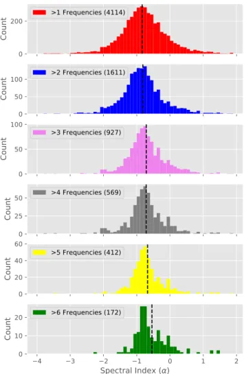
Finally, we estimate the radio spectral index for all sources in common and show their distribution in Fig-ure 11. There are 4114 sources found at only two frequen-cies (marked in red; Figure 11) and for those we estimate a mean α of –0.84. For 1611 sources that are found in three different catalogues (marked in blue; Figure 11) we found a mean α of –0.81 (SD=1.35). We also estimate the average
number hh mm ss (mJy) 1 00:07:36.88 –72:12:00.6 12.4 ± 1.3 3 2 00:09:47.69 –72:44:48.6 20.8 ± 2.1 3 3 00:10:24.52 –72:00:37.6 5.13 ± 0.56 2 4 00:10:28.35 –72:00:23.0 6.23 ± 0.66 2 5 00:11:58.28 –72:00:48.5 22.7 ± 2.3 3 6 00:12:47.55 –73:12:57.6 12.6 ± 1.3 3 7 00:14:25.83 –72:17:20.8 3.06 ± 0.35 3 8 00:14:31.23 –72:09:54.5 4.57 ± 0.48 3 9 00:15:09.85 –72:48:06.5 3.72 ± 0.40 2 10 00:15:24.82 –72:17:43.3 2.74 ± 0.32 2 −10 −5 0 5 10 ∆ Right Ascension (arcsec)
−10.0 −7.5 −5.0 −2.5 0.0 2.5 5.0 7.5 10.0 ∆ Declination (a rcsec) 0 200 Count 0 200 Count
Figure 7. Positional difference (MOST – ASKAP) of 1509 sources found in both the 843 MHz (MOST) and the 960 MHz catalogues. The mean offsets are ∆RA=+2.9000 (SD=2.65) and ∆DEC=–1.4500(SD=2.92).
α for sources that are detected in four (927 sources; pur-ple; Figure 11;α=–0.71, SD=0.75), five (569 sources; grey; Figure 11;α=–0.71, SD=0.59), six (412 sources; orange; Fig-ure 11; α=–0.67, SD=0.72) and seven (172 sources; green; Figure 11;α = −0.54, SD=0.51) different frequencies. Given that our sample sizes of SNRs, PNe and H ii regions are around 100-150 (see Sections 4 and 5), this distribution is as expected and indicates that the vast majority of our sources from Table 4 are most likely to be background objects (see e.g. Filipovi´c et al. 1998; Collier et al. 2018; Galvin et al. 2018). We note that some sources with flux density measure-ments at more than two frequencies might exhibit spectral curvature and therefore the fitted value of alpha would not represent a good estimate.
−10 −5 0 5 10
∆ Right Ascension (arcsec) −10.0 −7.5 −5.0 −2.5 0.0 2.5 5.0 7.5 10.0 ∆ Declination (a rcsec) 0 100 Count
Figure 8. Positional difference (ATCA – ASKAP) of 889 sources found in both the 1320 MHz and the 1400 MHz (ATCA) cata-logues. The mean offsets are
∆RA=–0.5800(SD=1.50) and ∆DEC=+1.0300(SD=1.95).
10−3 10−2 10−1 100
Flux Density MOST 843 MHz (Jy) 10−3 10−2 10−1 100 Flux Densit y ASKAP 960 MHz (Jy) 0 200 Count 0 200 Count
Figure 9. Integrated flux density comparison of sources found in both the 960 MHz and the 843 MHz catalogues. The best fit slope (linear) is 0.89±0.01 (dotted blue) while the red line repre-sent 1-to-1 ratio (see Section 3.3). The points are colour coded to indicate local density, yellow for high density through to purple for low density. The source integrated flux density distributions are shown in the side and top panels, with the black dashed line at the median integrated flux density.
10−3 10−2 10−1 100
Flux Density ATCA 1400 MHz (Jy) 10−3 10−2 10−1 100 Flux Densit y ASKAP 1320 MHz (Jy) 0 100 Count 0 100 Count
Figure 10. Integrated flux density comparison of sources found in both the 1320 MHz and the 1400 MHz catalogues. The best fit slope (linear) is 0.99±0.01 (dotted blue) while red line represent 1-to-1 ratio (see Section 3.3). The points are colour coded to in-dicate local density, yellow for high density through to purple for low density. The source integrated flux density distributions are shown in the side and top panels, with the black dashed line at the median integrated flux density.
4 ASKAP SMC SUPERNOVA REMNANT SAMPLE
Because of their proximity and location well away from the Galactic Plane, we are able to study the sources belonging to the MCs, such as the supernova semnant (SNR) population. Together, these galaxies offer the opportunity to produce a complete sample of SNRs suitable for population studies fo-cused on size, evolution, radio spectral index and beyond, as shown by Maggi et al. (2016) and Bozzetto et al. (2017). To that end, one of our prime goals with the next genera-tion of ASKAP surveys is to detect new and predominantly low surface brightness SNRs. Indeed, with its unique cov-erage and depth, this new ASKAP ESP survey allowed us to search for new SNRs and at the same time, measure the physical properties of the already established SNRs, exam-ples of which are shown in Figures 3 and 4.
Previous studies of SNRs in the SMC (Filipovi´c et al. 2005; Payne et al. 2007; Owen et al. 2011; Haberl et al. 2012b; Crawford et al. 2014; Roper et al. 2015; Alsaberi et al. 2019; Gvaramadze et al. 2019; Sano et al. 2019) have established 19 objects as bona-fide SNRs with two more con-sidered as good candidates. These two SNR candidates are not detected in our radio images and we will discuss them in our subsequent papers.
Here, we present our radio continuum study results which suggest two new sources to be SNR candidates (MCSNR J0057–7211 and MCSNR J0106–7242), bringing our sample of SMC SNRs and SNR candidates to 23. At the same time, we measure integrated flux densities for 18 of the 19 known SMC SNRs (see Table 7) and
0 200 C ou nt >1 Frequencies (4114) 0 50 100 C ou nt >2 Frequencies (1611) 0 50 100 C ou nt >3 Frequencies (927) 0 25 50 C ou nt >4 Frequencies (569) 0 20 40 60 C ou nt >5 Frequencies (412) 4 3 2 1 0 1 2 Spectral Index (α) 0 10 20 C ou nt >6 Frequencies (172)
Figure 11. Spectral index distribution of all sources in the field of SMC binned at 0.1. The vertical dashed line represents the meanα of each panel, as discussed in Section 3.3. The uppermost panel includes all the sources of the other panels beneath.
present our integrated flux density estimates for the two new SMC SNR candidates found in our new ASKAP SMC surveys (Table 8). An in-depth study of the SMC SNR population will be presented in Maggi et al. (submitted, https://arxiv.org/abs/1908.11234).
These two new SNR candidates were initially selected purely based on their typical morphological appearance (cir-cular shape). As our SMC SNR sample is morphologically diverse, various approaches (and initial parameters) were employed in order to measure the best SNR flux densities. Namely, we used the miriad (Sault et al. 1995) task imfit to extract integrated flux density, extensions (diameter/axes) and position angle for each radio detected SNR. For cross checking and consistency, we also used aegean and found no significant difference in integrated flux density estimates. We used two methods: For SNRs which are known point sources (such as SNR 1E 0102.2–7219, which is not resolved in radio) we use simple Gaussian fitting which produced the best result. The second approach was applied to all resolved SNRs. For those, we measured their local background noise (1σ) and carefully select the exact area of the SNR. We then estimated the sum of all brightnesses above 5σ of each
The two new SNR candidates are shown in Figs. 12 and 13 and their integrated flux density measurements in Ta-ble 8. These two new SNR candidates display approximately semi-circular structures consistent with a typical spherical morphology. As expected, they are both of low radio sur-face brightness, which is the main reason for their previous non-detection. We estimate the spectral index for both ob-jects (Table 8) and they are consistent with typical SNR spectra, as found in, for example, the larger Large Magel-lanic Cloud (LMC) population (see Fig. 13 in Bozzetto et al. 2017). Therefore, in addition to their typical morphology, their radio spectral index points to a non-thermal origin which further supports that these objects be classified as SNR candidates. Neither of these two SNR candidates are detected at optical or Infrared (IR) wave bands, which is not unusual given that a number of previously known bona-fide SNRs have only been seen at one wavelength (Filipovi´c et al. 2008).
New ASKAP SNR candidate MCSNR J0057−7211 (also see Ye et al. 1991) is located inside the ellipse around XMMU J0057.7–7213 (on the northern side, see Fig. 6 in Haberl et al. 2012b). The nearby point source XMMU J005802.4–721205 is listed as an Active Galac-tic Nuclei (AGN) candidate (Sturm et al. 2013). Also, there is a moderately bright, point-like X-ray source at 00:58:02.604, −72:12:06.7 with a non-thermal spectrum and LX∼ 1034 erg s−1 (Haberl et al. 2012b).
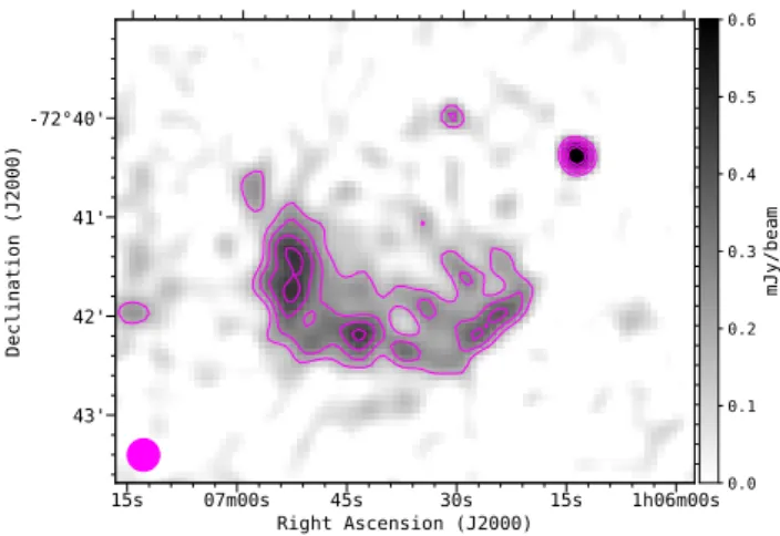
On inspection of present generation XMM–Newton mosaic images, we find diffuse emission at the posi-tion of the second ASKAP SMC SNR candidate – MC-SNR J0106−7242. A more comprehensive study of the whole SMC SNR population will be presented in an upcoming study by Maggi et al. (in prep.).
We also use the equipartition formulae2(Arbutina et al. 2012; Arbutina et al. 2013; Uroˇsevi´c et al. 2018) to esti-mate the magnetic field strength for these two SNR candi-dates. While this derivation is purely analytical, we empha-sise that it is formulated especially for the estimation of the magnetic field strength in SNRs. The average equipartition field over the whole shell of MCSNR J0057–7211 is ∼15µG while estimates for MCSNR J0106–7242 are around ∼8µG, with an estimated minimum energy3of Emin=6×1049erg and Emin=1.5×1049erg, respectively. These values are typical of
older SNRs at the end of the Sedov phase where the mag-netic field is three to four times more compressed than that of middle-age SNRs.
The position of these two SNR candi-dates on the surface brightness to diameter (Σ– D ) diagram (Σ= 6.38×10⁻²²W m−2Hz−1sr−1 and 5.38×10⁻²²W m−2Hz−1sr−1, D=47 pc and 44.9 pc, re-spectively) by Pavlovi´c et al. (2018), suggests that these
2 http://poincare.matf.bg.ac.rs/~arbo/eqp/
3 We use the following values: θ=1.370 and 1.290; κ = 0; S1 GHz=0.0307 Jy and 0.02363 Jy; and f=0.25.
0h57m36s 48s 58m00s 12s 24s Right Ascension (J2000) 13' 12' 11' De cl in at io n (J 20 0.0 0.2 0.4 0.6 0.8 mJ y/ be am
Figure 12. ASKAP ESP image of the new SMC SNR candi-date MCSNR J0057-7211 at 1320 MHz (grey scale and contours) smoothed to a resolution of 2000× 2000. Magenta contours are: 0.3, 0.5, and 0.7 mJy beam−1. The smoothed beam is shown as a filled magenta circle in the lower left corner. Two point-like sources in the lower right and left corner are unrelated background sources. The local RMS noise is 0.1 mJy beam−1.
1h06m00s 15s 30s 45s 07m00s 15s Right Ascension (J2000) 43' 42' 41' -72°40' De cl in at io n (J 20 00 ) 0.0 0.1 0.2 0.3 0.4 0.5 0.6 mJ y/ be am
Figure 13. ASKAP ESP image of the new low surface bright-ness SMC SNR candidate MCSNR J0106-7242 at 1320 MHz (grey scale and contours) smoothed to a resolution of 2000× 2000. Ma-genta contours are: 0.18, 0.27, 0.36, 0.45 and 0.54 mJy beam−1. The smoothed beam is shown as a filled magenta circle in the lower left corner. The point-like source in the upper right cor-ner is an unrelated background source. The local RMS noise is 0.06 mJy beam−1.
remnants are in the late Sedov phase, with an explosion energy of 1–2×1051erg, which evolves in an environment with a density of 0.02–0.2 cm−3.
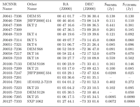
Table 7. 19 SNRs in the SMC. Only MCSNRJ0103–7201 is not detected in our ASKAP ESP images. The integrated flux density errors are<10 per cent. Column 2 (Other Name) abbreviations are: DEM S: Davies et al. (1976), [HFP2000]: Haberl et al. (2000), IKT: Inoue et al. (1983), SXP: Haberl et al. (2012a).
MCSNR Other RA DEC S960 MHz S1320 MHz
Name Name (J2000) (J2000) (Jy) (Jy)
J0041–7336 DEM S5 00 41 01.7 −73 36 30.4 0.138 0.130 J0046–7308 [HFP2000] 414 00 46 40.6 −73 08 14.9 0.111 0.110 J0047–7308 IKT 2 00 47 16.6 −73 08 36.5 0.441 0.381 J0047–7309 00 47 36.5 −73 09 20.0 0.201 0.185 J0048–7319 IKT 4 00 48 19.6 −73 19 39.6 0.121 0.092 J0049–7314 IKT 5 00 49 07.7 −73 14 45.0 0.068 0.060 J0051–7321 IKT 6 00 51 06.7 −73 21 26.4 0.085 0.096 J0052–7236 DEM S68 00 52 59.9 −72 36 47.0 0.091 0.081 J0058–7217 IKT 16 00 58 22.4 −72 17 52.0 0.079 0.070 J0059–7210 IKT 18 00 59 27.7 −72 10 09.8 0.559 0.502 J0100–7133 DEM S108 01 00 23.9 −71 33 41.1 0.161 0.146 J0103–7209 IKT 21 01 03 17.0 −72 09 42.5 0.100 0.085 J0103–7247 [HFP2000] 334 01 03 29.1 −72 47 32.6 0.0288 0.025 J0103–7201 01 03 36.6 −72 01 35.1 – – J0104–7201 1E 0102.2-7219 01 04 01.2 −72 01 52.3 0.402 0.272 J0105–7223 IKT 23 01 05 04.2 −72 23 10.5 0.102 0.095 J0105–7210 DEM S128 01 05 30.5 −72 10 40.4 – 0.050 J0106–7205 IKT 25 01 06 17.5 −72 05 34.5 0.0095 0.0090 J0127–7333 SXP 1062 01 27 44.1 −73 33 01.6 0.0072 0.0068
Table 8. Details of two new ASKAP SNRs candidates in the SMC. The integrated flux density errors are<10 per cent. N S abbreviation stands as at Henize (1956)
.
MCSNR Other RA DEC S960 MHz S1320 MHz α ± ∆α
Name Name (J2000) (J2000) (Jy) (Jy)
J0057–7211 N S66D 00 57 49.9 −72 11 47.1 0.030 0.0244 –0.75±0.04
J0106–7242 01 06 32.1 −72 42 17.0 0.024 0.020 –0.55±0.02
5 ASKAP SMC PLANETARY NEBULA SAMPLE
The location and proximity of the SMC also provides an op-portunity to create a complete sample of radio continuum detected planetary nebulae (PNe) in that nearby galaxy. PNe are important for studies of the chemical, atomic, molecular and solid-state galactic ISM enrichment (Kwok 2005, 2015). The next generation ASKAP surveys aim to provide detection of lower surface brightness planetary neb-ula (PN) to help complete the SMC PN sample.
Previous searches for radio PNe in the SMC (Payne et al. 2008; Filipovi´c et al. 2009; Bojiˇci´c et al. 2010; Lev-erenz et al. 2016) yielded 16 bona-fide PN detections. Our ASKAP ESP survey has revealed 6 new PN radio detections (see Table 9) reported here for the first time (Figure 14), bringing the total number of known SMC PNe detected in radio to 22. Our new data contribute 18 new accurate radio continuum flux density measurements from ASKAP on this sample (excluding dubious detections and upper flux limits), of which 7 are at 960 MHz and 11 at 1320 MHz.
All finding charts created here have been visually in-spected for a possible detection. Of 102 true, likely and pos-sible SMC PNe in our base catalogue we have matched 17
radio counterparts with peak emission over three times the local noise in the 1320 MHz map and 8 in the 960 MHz map. The flux densities were measured using the Gaussian fitting method imfit from casa4 (McMullin et al. 2007). Since none of the SMC PNe are expected to be resolved based on their known optical size, the Gaussian fitting was con-strained to the beam size, effectively measuring the peak of the emission. Calculations of uncertainties for this method are based on Condon (1997) and have been adopted directly from imfit’s output. We visually inspected all possible de-tections with a peak brightness over F ≥ 3σ using a com-parison between the original and the residual maps.
The results are presented in Table 9 and Figure 14. Out of 17 detections at 1320 MHz, we measured accurate flux densities for 11 PNe with peak brightness over 5σ. Like-wise, in the 960 MHz band we accurately measured 7 out of 8 detected PNe. We flagged PNe with the peak brightness below 5σ in Table 9 with a value in parentheses. The flux
4 We also used aegean, miriad and Selavy software packages to check for consistency and we found no noticeable discrepancy between various source finders.
able we apply free-free emission spectral energy modelling (Spectral Energy Distribution (SED); see further text), b) if only one or two data points were measured, we estimated the 5 GHz integrated flux density from the measurements at the frequency or frequencies available by applying a simple power law approximation i.e. S5GH z = Sν· (5/ν[GHz])−0.1.
For SED modelling we used a spherical shell model with a constant electron density in the shell (ne), outer radius
(Rout) and inner radius (Rin). The model can now be applied
to measured data points with:
Sν=4πkTeν 2 c2D2 R 2 out ∫ ∞ 0 x(1 − e−τν·g1(x))dx (1)
where τν is the optical thickness through the centre of the nebula at frequencyν which, for an assumption of ne= const
and a pure hydrogen isothermal plasma, can be approxi-mated withτν≈ 8.235 · 10−2Te−1.35ν−2.1n2e· 2(Rout− Rin). Fi-nally, the function g(x) describes the geometry of the nebula (see Olnon 1975, for more details). For this model g(x) has a form: g1(x)= p 1 − x2− q µ2− x2 for x< µ, =p 1 − x2 forµ ≤ x < 1 and = 0 for x ≥ 1, (2)
where µ = Rin/Rout i.e. inner to outer radii ratio. We fixed
the electron temperature to its canonical value (Te= 104 K)
and µ = 0.4 as this is found to be the expected average value for majority of Galactic PNe (Sch¨onberner et al. 2007; Marigo et al. 2001). With an assumed distance to the SMC of 60 kpc we fit the two free parameters, Routand the emission
measure (E M), through the centre of the nebula. Finally, the model shown here has been used to estimate the integrated flux density at 5 GHz.
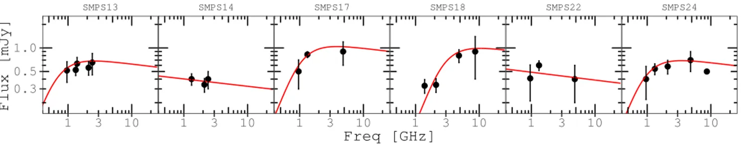
In Fig. 15 we show graphical results of the SED fitting. From the six PNe with an adequate number of data points to apply our spherical shell model, only four converged to acceptable values of Routand E M. For two PNe (SMP S14 and SMP S22) the model failed to converge and the data were fitted with the simple power law Sν∼να. The spectral indices (α) obtained are –0.09 and –0.1 for SMP S14 and SMP S22, respectively.
We present the modelled 5 GHz total flux densities in Table 9 (Column 11). The distribution of the modelled 5 GHz total flux densities for the detected sample is pre-sented in Fig. 16. It can be seen that the number of PNe drops down below 0.6 mJy which is approximately the de-tection limit for ASKAP ESP data. Objects detected be-low this limit are either upper limits or detections originat-ing from high sensitivity ATCA observations (Wong et al. 2011b). Therefore, we believe that our sample of radio de-tected SMC PNe is now complete down to ∼0.6 mJy. We have used this distribution to roughly estimate the number
would behave as F ∝ R(t)−3∝ t−3. Although simplistic, this approximation has proven to be quite effective in describ-ing changes in flux from Balmer lines durdescrib-ing the expansion phase in a large number of observationally constructed PN luminosity functions (Reid & Parker 2010; Ciardullo 2010). Using a sample of radio catalogued Galactic Bulge PNe, Bojiˇci´c (2010) showed that the theoretical shape of the PNLF (Ciardullo et al. 1989) effectively describes the distri-bution of radio flux densities of PNe at a known distance. Using our assumption that the SMC PN radio sample is now complete down to 0.6 mJy, we have used the theoreti-cal shape of the PNLF to estimate the distribution of 5 GHz integrated flux densities below the ASKAP ESP detection limit (more details in Bojiˇci´c et al. 2019, in prep.). We fit the truncated exponential function (Ciardullo et al. 1989) to the obtained distribution of log10(S5GHz) fluxes (in mJy).
The data is binned to 0.2 dex in log flux density and we have used only bins containing PNe with S5GHz > 0.6 mJy
for the fit. The estimated rough model is over-plotted on the resulting histogram (Figure 16; dashed line). Finally, we anticipate that increasing the sensitivity by an order of mag-nitude would allow detection of another 20 SMC PNe, while reaching a 10 µJy beam−1 (Norris et al. 2011) will allow us to increase the number of detections to ≈ 120 PNe i.e. over 50 per cent of the expected SMC PNe population (Jacoby & De Marco 2002).
6 OTHER INTERESTING SOURCES
In Sections 4 and 5 we investigated SNRs and PN popu-lations within the SMC. Large SMC H ii region complexes N 19 and N 66 are shown in Figures 3 and 4. Together with other SMC H ii regions and YSOs, they will be further in-vestigated in our subsequent papers.
We would also like to highlight some sources of inter-est behind the SMC that are worth following up. Due to their complex radio structure they are probes of galaxy in-teractions or interaction with the environment. These are presented in Figures 17, 18, 19, 20 and 21 and would fall into the category of extended radio AGN.
One of the most interesting sources behind the SMC re-vealed by our ASKAP observations is the radio AGN shown in Figure 17. This object displays a set of radio lobes asso-ciated to the an infrared IRAC source (background of Fig-ure 17). Also associated with the same source seems to be a radio jet with direction pointing towards the observer. Over the past year there has been a multi-wavelength effort to reveal of the true nature behind this peculiar radio struc-ture, which might be linked to a binary supermassive black hole. Still we cannot rule out chance coincidence. Sched-uled follow-up observations, with ATCA (PI: Vardoulaki) and SALT (PI: van Loon), will help shed light to the nature of this interesting radio source.
Other sources also show complex AGN structures with various morphological types (Figures 19 and 20) (see also
SMP S13 SMP S8 SMP S14 SMP S17 SMP S28 SMP S27 SMP S24 SMP S22 SMP S19 SMP S5 N E SMP S2
Figure 14. Finding charts of 11 SMC PNe with positive detection at 1320 MHz. Each field is 2 arcmin in size and the grey-scale uses the same sinh stretching. The approximate shape of the synthesized beam and orientation of each chart is displayed in the upper left corner. Red cross represents the catalogued position of a PN and green contours are radio continuum intensity at 3, 5, 8 and 12× RMS noise measured in the vicinity of the object. Here, we present only objects with 5σ detections for which we measured accurate flux densities. N is up and E is left in each panel.
SMPS13 SMPS14 SMPS17 SMPS18 SMPS22 SMPS24 1 3 10 1 3 10 1 3 10 1 3 10 1 3 10 1 3 10 0.3 0.5 1.0
Freq [GHz]
Flux [mJy]
Figure 15. Best fit model SEDs to the observed flux densities for 6 SMC PNe with three or more available and good data points.
0 5 10 −1.0 −0.5 0.0
log
10(S5GHz/mJy)
Number of PNe
Figure 16. Planetary nebulae luminosity function (PNLF) for the SMC. The dashed line represents the theoretical PNLF esti-mated assuming the sample is complete down to 0.6 mJy.
O’Brien et al. 2018) and sizes, including a bent source in a possible galaxy cluster (Figure 18). Such morphology of the extended radio emission, is expected from binary driven
jets. A similar configuration is also seen toward other Super Massive Black Hole (SMBH)s, such as OJ 287 (Kushwaha et al. 2019). The object in Figure 21 is a slightly bent FR-I type radio galaxy, possibly the central part of a Wide-Angle Tail (WAT) in a cluster of galaxies.
We also examined seven Flat Spectrum Radio Quasars (FSRQs) and BL Lacertae (BL-Lac) candidates from ˙ Zy-wucka et al. (2018) in our radio catalogues. We found that objects J0111−7302 (proposed BL-Lac5.; Figure 23) and possibly J0120−7334 (proposed FSRQs; Figure 22) ex-hibit typical FR-I morphology with complex but steep spec-tral indices which would argue for their AGN nature. The other five sources listed in ˙Zywucka et al. (2018) are point-like radio sources in our catalogues: J0039−7356 (BL-Lac; α = −1.1), J0054−7248 (FSRQs; detected only at 1320 MHz), J0114−7320 and J0122−7152 (both proposed FSRQs but we detect as a complex AGN with jets) and J0123−7236 (BL-Lac;α = −0.7). In addition, we found four radio sources in our catalogue that correspond to the Visual and Infrared
5 We note that BL-Lac’s with large extents are assumed to be compact which is in contrast to this object. We also note that, for example, Hern´andez-Garc´ıa et al. (2017) show several known extended (even giant) BL-Lac
(mJy) (mJy) (mJy) (mJy) (mJy) (mJy) (mJy) (mJy) (1) (2) (3) (4) (5) (6) (7) (8) (9) (10) (11) SMP S2† 00:32:39 −71:41:59.5 ... ... ... ... (2) 1.25±0.08 1.1±0.2 1.1 SMP S3† 00:34:22 −73:13:21.5 ... ... ... ... ... (0.3) (0.4) 0.3 SMP S5† 00:41:22 −72:45:16.8 ... ... ... ... ... 0.67±0.08 0.3±0.2 0.6 SMP S6 00:41:28 −73:47:06.4 1.1±0.5 1.3±0.1 ... ... >0.2 ... ... 1.2 SMP S8† 00:43:25 −72:38:18.8 ... ... ... ... ... 0.43±0.08 ... 0.4 SMP S9 00:45:21 −73:24:10.0 ... ... ... 0.15 ... ... ... 0.1 SMP S10† 00:47:00 −72:49:16.6 ... ... ... ... (0.3) (0.4) ... 0.2 SMP S13† 00:49:52 −73:44:21.7 ... ... 0.7±0.2 0.56 ... 0.52±0.08 0.52±0.15 0.6 SMP S14† 00:50:35 −73:42:57.9 ... ... 0.4±0.1 0.34 ... 0.40±0.06 ... 0.4 SMP S16† 00:51:27 −72:26:11.7 ... 0.6±0.1 ... ... ... <0.4 ... 0.6 J18 00:51:43 −73:00:54.5 ... ... 0.24 ... ... ... ... 0.2 SMP S17† 00:51:56 −71:24:44.2 ... 0.9±0.3 ... ... ... 0.82±0.07 0.5±0.2 0.9 SMP S18† 00:51:58 −73:20:31.9 0.9±0.5 0.8±0.15 ... 0.34 0.3 (0.3) ... 0.8 SMP S19† 00:53:11 −72:45:07.6 ... ... 0.6±0.2 ... ... 0.36±0.08 ... 0.6 MA891 00:55:59 −72:14:00.3 ... ... ... 0.92 ... ... ... 0.8 LIN 302† 00:56:19 −72:06:58.5 ... ... ... 0.11 ... (0.3) ... 0.1 SMP S21 00:56:31 −72:27:02.0 ... ... ... 0.21 ... ... ... 0.2 SMP S22† 00:58:37 −71:35:48.8 ... 0.4±0.2 ... ... ... 0.60±0.08 0.4±0.2 0.4 SMP S23† 00:58:42 −72:56:59.9 ... ... ... ... ... (0.4) ... 0.3 SMP S24† 00:59:16 −72:01:59.8 0.5 0.7±0.2 ... 0.58 ... 0.54±0.09 0.4±0.2 0.7 SMP S27† 01:21:11 −73:14:34.8 ... ... ... ... ... 0.88±0.08 0.68±0.10 0.8 SMP S28† 01:24:12 −74:02:32.3 ... ... ... ... ... 0.32±0.07 ... 0.3
Survey Telescope for Astronomy (VISTA; Emerson et al. 2006), survey of the MCs (VMC; Cioni et al. 2011) and spec-troscopically confirmed quasars (Ivanov et al. 2016). They are J0027−7223 (S1320 MHz=0.265 mJy), J0029−7146 (α = −1.0), J0035−7201 (α = −0.5) and J0119−7348 (α = −0.8). While small, this sample exhibits steep spectral indices typ-ical of the majority of background radio objects.
Finally, we note a radio detection of an ultra-bright sub-millimeter galaxy MM J01071−7302 (Takekoshi et al. 2013) and found a steep spectrum withα = −0.9.
In total, we found 7736 point radio sources with fluxes over 5 times the local noise, the vast majority of which are likely to be in the background of the SMC. Through absorp-tion measurements, all these sources can provide excellent probes for the study of cold gas in both SMC and the Galaxy (e.g. Li et al. 2018; McClure-Griffiths et al. 2015; Dickey et al. 2013). A more detailed analysis of these background sources will be presented in Pennock et al. (in prep.).
7 CONCLUSIONS
In this paper we present the ASKAP EMU ESP radio con-tinuum survey of the SMC taken at 960 MHz and 1320 MHz. Our findings can be summarised as follows:
• This new ASKAP survey is a significant improvement (factor of ∼4 in the median RMS) compared to previous ATCA/MOST surveys of the SMC.
• We identify 4489 and 5954 point sources at 960 MHz and 1320 MHz, respectively (Tables 2 and 3), with the ma-jority of these sources detected above the 5σ threshold in their respective bands. We also list non-point sources at both ASKAP frequencies in Tables 5 and 6 (282 and 641, respec-tively).
• Combining our two new ASKAP catalogues with other radio continuum surveys, we found 7736 point-like sources in common which we list in Table 4, together with spectral indices we determined from all available survey data.
• Two new low surface brightness SNR candidates were discovered, bringing the total number of SNRs and SNR candidates in the SMC to 23.
• Radio counterparts to 22 optically known PNe were de-tected. This sample of PNe is complete down to 0.6 mJy.
ACKNOWLEDGEMENTS
The Australian SKA Pathfinder (ASKAP) are part of the Australian Telescope which is funded by the Commonwealth of Australia for operation as National Facility managed by CSIRO. We used the karma and miriad software pack-ages developed by the Australia Telescope National Facil-ity (ATNF). Operation of ASKAP is funded by the Aus-tralian Government with support from the National Col-laborative Research Infrastructure Strategy. ASKAP uses the resources of the Pawsey Supercomputing Centre. Es-tablishment of ASKAP, the Murchison Radio–astronomy Observatory and the Pawsey Supercomputing Centre are initiatives of the Australian Government, with support from the Government of Western Australia and the Sci-ence and Industry Endowment Fund. We acknowledge the Wajarri Yamatji people as the traditional owners of the Observatory site. T.D.J. acknowledges support for this re-search from a Royal Society Newton International Fellow-ship, NF171032. M.J.M. acknowledges the support of the National Science Centre, Poland, through the SONATA BIS grant 2018/30/E/ST9/00208. The National Radio Astron-omy Observatory is a facility of the National Science
Foun-1h02m00s
20s
40s
03m00s
20s
40s
Right Ascension (J2000)
41'
40'
39'
38'
37'
-70°36'
De
cl
in
at
io
n
(J
20
00
)
Figure 17. ASKAP ESP image (contours) of the possible double black hole AGN. The background image is a three-colour IRAC composite with 8.0, 4.5 and 3.6µm represented as red, green and blue, respectively. The magenta radio contours are from our 1320 MHz survey drawn at 0.25, 0.3, 0.5, 0.7, 1, 1.5, 2, 3 and 5 mJy beam−1. The 1320 MHz radio beam size of 16.300× 15.100is shown as a filled magenta ellipse in the lower left corner.
dation operated under cooperative agreement by Associated Universities, Inc. Partial support for L.R. comes from U.S. National Science Foundation grant AST1714205 to the Uni-versity of Minnesota. Project/paper is partially supported by NSFC No. 11690024, CAS International Partnership No. 114A11KYSB20160008. This work is part of the project 176005 “Emission nebulae: structure and evolution” sup-ported by the Ministry of Education, Science, and Techno-logical Development of the Republic of Serbia. H.A. bene-fited from project CIIC 218/2019 of University of Guanaju-ato. The authors would like to thank the anonymous referee for a constructive report and useful comments.
REFERENCES
Alsaberi R. Z. E., et al., 2019, MNRAS, 486, 2507
Arbutina B., Uroˇsevi´c D., Andjeli´c M. M., Pavlovi´c M. Z., Vukoti´c B., 2012, The Astrophysical Journal, 746, 79
Arbutina B., Uroˇsevi´c D., Vuˇceti´c M. M., Pavlovi´c M. Z., Vukoti´c B., 2013, ApJ, 777, 31
Bojiˇci´c I., 2010, PhD thesis, Macquarie University
Bojiˇci´c I. S., Filipovi´c M. D., Crawford E. J., 2010, Serbian As-tronomical Journal, 181, 63
Bozzetto L. M., et al., 2017, ApJS, 230, 2
Ciardullo R., 2010, Publ. Astron. Soc. Australia, 27, 149 Ciardullo R., Jacoby G. H., Ford H. C., Neill J. D., 1989, ApJ,
339, 53
Cioni M.-R. L., et al., 2011, A&A, 527, A116 Clarke J. N., 1976, MNRAS, 174, 393
Collier J., 2016, PhD thesis, Western Sydney University (Aus-tralia
Collier J. D., et al., 2018, MNRAS, 477, 578 Condon J. J., 1997, PASP, 109, 166
Cornwell T. J., Humphreys B., Lenc E., Voronkov M., Whiting M. T., 2011, Technical Report 028, Askap-sw-0020: ASKAP science processing
Crawford E. J., Filipovi´c M. D., de Horta A. Y., Wong G. F., Tothill N. F. H., Draskovic D., Collier J. D., Galvin T. J., 2011, Serbian Astronomical Journal, 183, 95
Crawford E. J., Filipovi´c M. D., McEntaffer R. L., Brantseg T., Heitritter K., Roper Q., Haberl F., Uroˇsevi´c D., 2014, AJ, 148, 99
Davies R. D., Elliott K. H., Meaburn J., 1976, Mem. RAS, 81, 89 DeBoer D. R., et al., 2009, IEEE Proceedings, 97, 1507
Di Teodoro E. M., et al., 2019, MNRAS, 483, 392
Dickey J. M., et al., 2013, Publ. Astron. Soc. Australia, 30, e003 Emerson J., McPherson A., Sutherland W., 2006, The Messenger,
126, 41
Filipovi´c M. D., Jones P. A., White G. L., Haynes R. F., Klein U., Wielebinski R., 1997, A&AS, 121, 321
Filipovi´c M. D., Haynes R. F., White G. L., Jones P. A., 1998, A&AS, 130, 421
Filipovi´c M. D., Bohlsen T., Reid W., Staveley-Smith L., Jones P. A., Nohejl K., Goldstein G., 2002, MNRAS, 335, 1085 Filipovi´c M. D., Payne J. L., Reid W., Danforth C. W.,
1h33m00s 30s 34m00s 30s 35m00s Right Ascension (J2000) 20' 19' 18' De cl in at io n
Figure 18. ASKAP ESP image (contours) shows a long, twisted structure that appears to be a highly distorted tailed radio galaxy associated with 2MASX J01342297–7318113, a bright galaxy (V=15.9 mag) without spectroscopic redshift. Although the mul-tiple bends might suggest that there is actually more than one radio source, there is no obvious second optical/IR host. The bright compact object near the centre of the radio source elon-gated E-W and ∼3 arcmin W of 2MASX J01342297–7318113, is 2MASS J01334172–7317527, but GaiaDR2 (Gaia Collaboration et al. 2018) shows it to be a star with significant parallax and proper motion. The background image is a three-colour IRAC composite with 8.0, 4.5 and 3.6 µm represented as red, green and blue, respectively. The magenta radio contours are from our 1320 MHz survey drawn at 0.25, 0.3, 0.5, 0.7, 1, 1.5, 2, 3 and 5 mJy beam−1. The 1320 MHz beam size of 16.300× 15.100is shown as a filled magenta ellipse in the lower left corner.
1h38m10s 20s 30s 40s Right Ascension (J2000) 37' 36' -72°35' De cl in at io n (J 20 00 )
Figure 19. ASKAP ESP image of the “duck” AGN complex or possible bent-tail radio galaxy. The background image is a three-colour IRAC composite with 8.0, 4.5 and 3.6µm represented as red, green and blue, respectively. The magenta radio contours are from our 1320 MHz survey drawn at 0.25, 0.3, 0.5, 0.7, 1, 1.5, 2, 3 and 5 mJy beam−1. The 1320 MHz beam size of 16.300× 15.100is shown as a filled magenta ellipse in the lower left corner.
Science, 307, 1610
Gaia Collaboration et al., 2018, A&A, 616, A1 Galvin T. J., et al., 2018, MNRAS, 474, 779 Gordon K. D., et al., 2011, AJ, 142, 102
Gvaramadze V. V., Kniazev A. Y., Oskinova L. M., 2019, MN-RAS, 485, L6
Haberl F., Filipovi´c M. D., Pietsch W., Kahabka P., 2000, A&AS, 142, 41
Haberl F., Sturm R., Filipovi´c M. D., Pietsch W., Crawford E. J., 2012a, A&A, 537, L1
Haberl F., et al., 2012b, A&A, 545, A128
Hancock P. J., Murphy T., Gaensler B. M., Hopkins A., Curran J. R., 2012, Aegean: Compact source finding in radio images, Astrophysics Source Code Library (ascl:1212.009)
Hancock P. J., Trott C. M., Hurley-Walker N., 2018, Publ. Astron. Soc. Australia, 35, e011
Haynes R. F., Klein U., Wielebinski R., Murray J. D., 1986, A&A, 159, 22
Henize K. G., 1956, ApJS, 2, 315
Henize K. G., Westerlund B. E., 1963, ApJ, 137, 747 Hern´andez-Garc´ıa L., et al., 2017, A&A, 603, A131
Hilditch R. W., Howarth I. D., Harries T. J., 2005, MNRAS, 357, 304
Hotan A. W., et al., 2014, Publ. Astron. Soc. Australia, 31, e041 Inoue H., Koyama K., Tanaka Y., 1983, in Danziger J., Gorenstein P., eds, IAU Symposium Vol. 101, Supernova Remnants and their X-ray Emission. pp 535–540
Ivanov V. D., et al., 2016, A&A, 588, A93 Jacoby G. H., De Marco O., 2002, AJ, 123, 269
Johnston S., et al., 2008, Experimental Astronomy, 22, 151 Kushwaha P., de Gouveia Dal Pino E. M., Gupta A. C., Wiita
P. J., 2019, arXiv e-prints,
Kwok S., 2005, Journal of Korean Astronomical Society, 38, 271 Kwok S., 2015, Highlights of Astronomy, 16, 623
Leverenz H., Filipovi´c M. D., Bojiˇci´c I. S., Crawford E. J., Collier J. D., Grieve K., Draˇskovi´c D., Reid W. A., 2016, Ap&SS, 361, 108
Leverenz H., Filipovi´c M. D., Vukoti´c B., Uroˇsevi´c D., Grieve K., 2017, MNRAS, 468, 1794
Li D., et al., 2018, ApJS, 235, 1 Maggi P., et al., 2016, A&A, 585, A162
Mao S. A., Gaensler B. M., Stanimirovi´c S., Haverkorn M., McClure-Griffiths N. M., Staveley-Smith L., Dickey J. M., 2008, ApJ, 688, 1029
Mao S. A., et al., 2012, ApJ, 759, 25
Marigo P., Girardi L., Groenewegen M. A. T., Weiss A., 2001, A&A, 378, 958
Mauch T., Murphy T., Buttery H. J., Curran J., Hunstead R. W., Piestrzynski B., Robertson J. G., Sadler E. M., 2003, MNRAS, 342, 1117
McClure-Griffiths N. M., et al., 2015, Advancing Astrophysics with the Square Kilometre Array (AASKA14), p. 130 McClure-Griffiths N. M., et al., 2018, Nature Astronomy, 2, 901 McConnell D., 2017, Technical report, ACES memo 15:
Observ-ing with ASKAP: Optimisation for survey speed. CSIRO Aus-tralia Telescope National Facility
McConnell D., et al., 2016, Publ. Astron. Soc. Australia, 33, e042 McGee R. X., Newton L. M., Butler P. W., 1976, Australian
Jour-nal of Physics, 29, 329
0h20m00s
30s
21m00s
30s
Right Ascension (J2000)
24'
23'
22'
21'
20'
-73°19'
De
cl
in
at
io
n
(J
20
00
)
Figure 20. ASKAP ESP image of the FR-II AGN. The background image is a three-colour IRAC composite with 8.0, 4.5 and 3.6µm represented as red, green and blue, respectively. The magenta radio contours are from our 1320 MHz survey drawn at 0.25, 0.3, 0.5, 0.7, 1, 1.5, 2, 3 and 5 mJy beam−1. The 1320 MHz beam size of 16.300× 15.100is shown as a filled magenta ellipse in the lower left corner.
1h04m30s 40s 50s 05m00s 10s Right Ascension (J2000) 22' 21' -70°20' De cl in at io n (J 20 00 )
Figure 21. ASKAP ESP image of the FR-I AGN. The back-ground image is a three-colour IRAC composite with 8.0, 4.5 and 3.6µm represented as red, green and blue, respectively. The ma-genta radio contours are from our 1320 MHz survey drawn at 0.25, 0.3, 0.5, 0.7, 1, 1.5, 2, 3 and 5 mJy beam−1. The 1320 MHz beam size of 16.300× 15.100is shown as a filled magenta ellipse in the lower left corner.
2007, in Astronomical data analysis software and systems XVI. p. 127
Meixner M., et al., 2006, AJ, 132, 2268 Middelberg E., et al., 2008, AJ, 135, 1276
Murphy T., et al., 2013, Publ. Astron. Soc. Australia, 30, e006 Norris R. P., et al., 2006, AJ, 132, 2409
Norris R. P., et al., 2011, Publ. Astron. Soc. Australia, 28, 215 O’Brien A. N., Norris R. P., Tothill N. F. H., Filipovi´c M. D.,
2018, MNRAS, 481, 5247 1h20m40s 50s 21m00s 10s Right Ascension (J2000) 36' 35' -73°34' De cl in at io n (J 20 00 )
Figure 22. ASKAP ESP image of the possible AGN J0120−7334. The background image is a three-colour IRAC composite with 8.0, 4.5 and 3.6µm represented as red, green and blue, respectively. The yellow radio contours are from our 1320 MHz survey drawn at 0.25, 0.3, 0.5, 1, 2, 3, 5, 10, 20 and 30 mJy beam−1. The 1320 MHz beam size of 16.300× 15.100is shown as a filled magenta ellipse in the lower left corner.
Oliveira J. M., et al., 2013, MNRAS, 428, 3001 Olnon F. M., 1975, A&A, 39, 217
Owen R. A., et al., 2011, A&A, 530, A132
1h11m00s
20s
40s
12m00s
Right Ascension (J2000)
04'
03'
02'
-73°01'
De
cl
in
at
io
n
(J
20
00
)
Figure 23. ASKAP ESP image of the AGN complex J0111−7302. The background image is a three-colour IRAC composite with 8.0, 4.5 and 3.6µm represented as red, green and blue, respectively. The yellow radio contours are from our 1320 MHz survey drawn at 0.25, 0.3, 0.5, 1, 2, 3, 5, 10, 20, 30 and 50 mJy beam−1. The 1320 MHz beam size of 16.300× 15.100is shown as a filled magenta ellipse in the lower left corner.
Filipovi´c M. D., 2018, ApJ, 852, 84
Payne J. L., Filipovi´c M. D., Reid W., Jones P. A., Staveley-Smith L., White G. L., 2004, MNRAS, 355, 44
Payne J. L., White G. L., Filipovi´c M. D., Pannuti T. G., 2007, MNRAS, 376, 1793
Payne J. L., Filipovi´c M. D., Crawford E. J., de Horta A. Y., White G. L., Stootman F. H., 2008, Serbian Astronomical Journal, 176, 65
Pietrzy´nski G., et al., 2019, Nature, 567, 200 Reid W. A., Parker Q. A., 2010, MNRAS, 405, 1349
Reid W. A., Payne J. L., Filipovi´c M. D., Danforth C. W., Jones P. A., White G. L., Staveley-Smith L., 2006, MNRAS, 367, 1379
Roper Q., McEntaffer R. L., DeRoo C., Filipovi´c M., Wong G. F., Crawford E. J., 2015, ApJ, 803, 106
Sano H., et al., 2019, arXiv e-prints,
Sault R. J., Teuben P. J., Wright M. C. H., 1995, in Shaw R. A., Payne H. E., Hayes J. J. E., eds, Astronomical Society of the Pacific Conference Series Vol. 77, Astronomical Data Analysis Software and Systems IV. p. 433 (arXiv:astro-ph/0612759) Sch¨onberner D., Jacob R., Steffen M., Sandin C., 2007, A&A,
473, 467
Sturm R., et al., 2013, A&A, 558, A3 Takekoshi T., et al., 2013, ApJ, 774, L30
Turtle A. J., Ye T., Amy S. W., Nicholls J., 1998, Publ. Astron. Soc. Australia, 15, 280
Uroˇsevi´c D., Pavlovi´c M. Z., Arbutina B., 2018, The Astrophysical Journal, 855, 59
Winkler P. F., et al., 2005, in American Astronomical Society Meeting Abstracts. p. 1380
Wong G. F., Filipovi´c M. D., Crawford E. J., de Horta A. Y.,
Galvin T., Draskovic D., Payne J. L., 2011a, Serbian Astro-nomical Journal, 182, 43
Wong G. F., et al., 2011b, Serbian Astronomical Journal, 183, 103
Wong G. F., et al., 2012a, Serbian Astronomical Journal, 184, 93 Wong G. F., Filipovi´c M. D., Crawford E. J., Tothill N. F. H., De Horta A. Y., Galvin T. J., 2012b, Serbian Astronomical Journal, 185, 53
Wright A., Otrupcek R., 1990, in PKS Catalog (1990).
Ye T., Turtle A. J., Kennicutt R. C. J., 1991, MNRAS, 249, 722 ˙
Zywucka N., Goyal A., Jamrozy M., Stawarz L., Ostrowski M., Koz lowski S., Udalski A., 2018, ApJ, 867, 131
This paper has been typeset from a TEX/LATEX file prepared by the author.