Alma Mater Studiorum – Università di Bologna
DOTTORATO DI RICERCA IN
INGEGNERIA CIVILE E AMBIENTALE
Ciclo XXVI
Settore Concorsuale di afferenza: 08/A1 Settore Scientifico disciplinare: ICAR/01
WAVE DRIVEN DEVICES FOR THE
OXYGENATION OF BOTTOM LAYERS
Presentata da:
Alessandro Antonini
Coordinatore Dottorato
Relatore
Chiar.mo Prof. Alberto Lamberti
Chiar.mo Prof. Alberto Lamberti
ii
ACKNOWLEDGMENTS
Questo capitolo della tesi esula notevolmente dagli altri e da tutto il resto del lavoro. In questa sezione vorrei ringraziare chi, in un modo o in un altro, mi è stato vicino e d’aiuto in questo percorso. Si tratta di parole e non di numeri o fenomeni fisici e vista la mia mancanza in questo ambito, così distante dall’ingegneria, spero che tutte le persone che non sono citate o ringraziate a dovere non se ne abbiano a male.
Sono passati tre anni, intensi ed entusiasmanti dove sono state poche le volte, se non forse nessuna, in cui è stato un peso per me alzarmi e andare a lavorare. E questo, credo, sia una cosa impagabile, con nessun tipo stipendio o alcuna posizione prestigiosa.
Per questo, il primo e più doveroso ringraziamento va al mio tutor, Professore Alberto Lamberti, che in un’estate di circa quattro anni fa si vide arrivare in ufficio uno sconosciuto che gli chiedeva di fargli da tutor durante il periodo di dottorato. Per la fiducia dimostrata, da quel giorno sino ad oggi, e per il continuo supporto in tutte le attività che ho portato avanti durante il dottorato, non posso che esprimergli la mia più totale gratitudine.
Una seconda importante figura di questo dottorato è stata la Professoressa Renata Archetti, che è stata presente ogni volta in cui ho avuto bisogno; rivolgendosi a me sempre con il sorriso. Vorrei rivolgerle un grazie particolare e doveroso per avermi coinvolto in numerose attività, dandomi la possibilità di lavorare con nuove persone e con altri gruppi di ricerca.
Un ringraziamento va poi alla Professoressa Nadia Pinardi, che ha reso possibile un periodo della mia vita che non potrò mai dimenticare, quello newyorkese. E’ proprio durante quei sei mesi passati allo Stevens Institute of Technology che ho conosciuto delle persone stupende, che mi hanno accolto nel loro laboratorio con entusiasmo ed affetto. Per questo, un caloroso ringraziamento lo devo al Professor Alan Blumberg ed al Professor Len Imas che mi hanno messo a disposizione le loro conoscenze e le loro strutture. Inoltre, non posso che ringraziare anche i ragazzi dell’aula studenti al Davidson
iii
Laboratory: Javier, i tuoi consigli mi hanno cambiato molto. Larry, Bin, Gong avete reso quei giorni ancora più piacevoli di quello che potevano essere.
Infine, un grazie speciale non può che andare ai miei genitori, che hanno fatto si che io sia quello che sono ora; ma soprattutto ad Agnese che mi è sempre stata vicina e ha sopportato con pazienza il mio andare e tornare da Bologna.
Con affetto
iv
ABSTRACT
Counteract one of the most urgent environmental issues in estuarine and coastal ecosystems as eutrophication, hypoxia and anoxia is a main goal for many countries around the world. According to the European Union, developing new projects to preserve native species, habitat and ecological and biological processes in coastal areas is a priority action sector for the Italian government.
This thesis discusses the design of a system to use wave energy to pump oxygen-rich surface water towards the bottom of the sea.
A simple device, called OXYFLUX, is proposed in a scale model and tested in a wave flume in order to validate its supposed theoretical functioning.
Once its effectiveness has been demonstrated, a overset mesh, CFD model has been developed and validated by means of the physical model results. Both numerical and physical results show how wave height affects the behavior of the device. Wave heights lower than about 0.5 m overtop the floater and fall into it. As the wave height increases, phase shift between water surface and vertical displacement of the device also increases its influence on the functioning mechanism. In these situations, with wave heights between 0.5 and 0.9 m, the downward flux is due to the higher head established in the water column inside the device respect to the outside wave field. Furthermore, as the wave height grows over 0.9 m, water flux inverts the direction thanks to depression caused by the wave crest pass over the floater. In this situation the wave crest goes over the float but does not go into it and it draws water from the bottom to the surface through the device pipe. By virtue of these results a new shape of the floater has been designed and tested in CFD model. Such new geometry is based on the already known Lazzari’s profile and it aims to grab as much water as possible from the wave crest during the emergence of the floater from the wave field. Results coming from the new device are compared with the first ones in order to identify differences between the two shapes and their possible areas of application.
v
TABLE OF CONTENTS
Chapter Page ACKNOWLEDGMENTS ... ii ABSTRACT ... iv TABLE OF CONTENTS ... v LIST OF TABLES ... xiLIST OF FIGURES ... xiii
CHAPTER I: Introduction ... 1
A common worldwide problem: eutrophication and hypoxia ... 1
What is the hypoxia ... 2
Consequence of the eutrophication ... 3
Nutrients, eutrophication and hypoxia: an overview on the connections ... 5
Locations of global eutrophic and hypoxic areas ... 7
Wave Energy Converter, Strengths and weaknesses ... 9
History of the Ocean Wave Energy Converters ... 9
Strengths and weaknesses of the Wave Energy Converter ... 11
CHAPTER II: Literature Survey ... 14
vi
Anoxia in the northern Adriatic ... 16
Water mass structure: temperature, salinity, dissolved oxygen and stratification of the North Adriatic Sea ... 17
Temperature and Salinity ... 19
Dissolved oxygen ... 20
Wave climate of North Adriatic ... 22
Wave Overtopping ... 26
Wave overtopping studies: present knowledge ... 27
Influence of slope angle ... 30
Influence of draft... 30
Influence of dimensionless freeboard parameter (R) ... 32
Wave energy as a propellant for sea water pump ... 34
Overtopping wave energy converters ... 36
Devices to counteract oxygen depletion ... 40
Purpose of the study ... 43
CHAPTER III: Development of the device OXYFLUX ... 45
Proof of concept ... 47
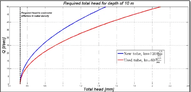
Required head ... 48
Construction of the model ... 52
vii
Tube ... 56
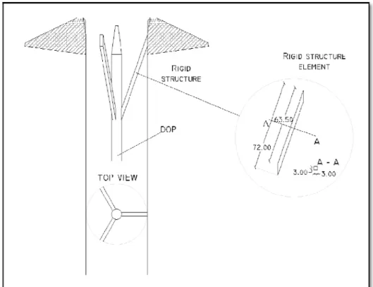
Stabilizing ring ... 56
CHAPTER IV: Physical investigation ... 62
Parameters investigated ... 62
Device’s structures ... 62
Modification of the mooring system ... 64
Modification of the crest freeboard ... 64
Laboratory set-up ... 65
Measurement of the displacement ... 69
Image processing procedure ... 69
Semi manual approach ... 70
Automatic approach ... 76
Results ... 82
Calm water tests: hydrodynamic parameters ... 82
Motion analysis ... 86
Water velocity measurements ... 95
The used key features of Signal Processing's DOP2000 velocimeter ... 96
The Emitting Frequency ... 96
Pulse repetition frequency ... 97
viii
Burst length ... 99
Resolution ... 99
Number of gates ... 100
Emitting Power and Sensitivity ... 100
Number of Emissions Per Profile ... 101
Profiles to record ... 102
Measurement set-up ... 103
Results ... 103
CHAPTER V: Numerical investigation ... 111
Governing equation ... 112
Discretization: Finite Volume Method (FVM) ... 113
Discrete form of momentum equation ... 113
Discrete form of continuity equation ... 114
SIMPLE Solver Algorithm ... 116
Multigrid Methods ... 117
Multiphase Methods... 119
VOF Multiphase Model ... 120
Turbulence model ... 122
Response calculation ... 124
ix
Parameters of the solver ... 126
Solution convergence ... 128
Fixed mesh technique ... 129
Domain and boundary conditions ... 129
Mesh and time step selection ... 132
Results ... 135
Overset mesh technique ... 140
Domain and boundary conditions ... 143
Mesh and time step selection ... 147
Results and model validation ... 154
CHAPTER VI: DEVELOPMENT AND NUMERICAL MODELLING OF THE NEW GEOMETRY ... 165
Floater of Geometry 2 ... 167
Numerical modelling and results of Geometry 2 ... 172
Results ... 174
CHAPTER VII: DISCUSSION ... 177
CHAPTER VIII: CONCLUSION ... 182
Physical Modelling: Conclusions ... 183
Numerical Modelling: Conclusions ... 184
x
Final remarks ... 186
REFERENCES ... 187
Appendix A ... 205
xi
LIST OF TABLES
Table Page Table 1: Average monthly and annual wave power significant wave heights (m), Tr return
period (years), [58]... 23
Table 2: Average monthly and annual wave power (kw/m), [58]. ... 25
Table 3: Average Summer density anomaly in North Adriatic, [46]. ... 48
Table 4: Froude scale law ... 53
Table 5: Hydrodynamics parameters of the floater. ... 55
Table 6: Results of reflection analysis for 49 tested wave state, (subscripts t, m_i, m_r indicate target, medium incident, medium reflected) ... 67
Table 7: Hydrodynamic parameters ... 86
Table 8: Solver configuration for all simulations. ... 128
Table 9: Regular wave states simulated. ... 140
Table 10: grid characteristics. ... 151
Table 11: Regular wave states simulated in numerical tank. ... 155
Table 12: Geometric parameters used for Geometry 2. ... 169
Table 13: Hydrodynamics parameters of the Geometry 2 floater. ... 170
Table 14: Regular wave states simulated in numerical tank and results for Geometry 2. ... 174
xiii
LIST OF FIGURES
Figure Page
Figure 1: Comparative evaluation of fishery response to nutrients,[18]. ... 7
Figure 2: World hypoxic and eutrophic coastal areas, [8]. ... 9
Figure 3: Schematic representation of Backward Bent Duct Buoy, [21]. ... 11
Figure 4: Adriatic Sea coastline an topography, [40]. ... 14
Figure 5: Adriatic Sea general circulations,[41]. ... 16
Figure 6: Monthly mean heat flux at the surface (W/m2), estimations based on 4 different datasets,[40]. ... 18
Figure 7: Seasonal climatological profile of Adriatic, a) Northern Adriatic, b) Middle Adriatic, c) Southern Adriatic. The variables represent are Temperature, °C, (left); and Salinity, ppm, (right). Spring , summer , autumn , winter , [40]. ... 20
Figure 8: Seasonal climatological profile of Adriatic: a) Northern Adriatic shallower or equal to 50 m, b) northern Adriatic deeper than 50 m, c) middle Adriatic, d) southern Adriatic max depth, e) southern Adriatic shallower or equal to 300 m. Dissolved oxygen (ml/l). Spring , summer , autumn , winter , [40]. ... 21
Figure 9: Locations of the platform Panon and Labin, [54]. ... 22
Figure 10: Location of the IWN buoys, [58]. ... 24
Figure 11: Wave overtopping of the Wave Dragon prototype,[60]. ... 26
Figure 12: Parameters investigated by Kofoed,[62]. ... 29
Figure 13: λα as a function of the slope angle. Value for tested shape in present work is black circle. ... 30
xiv
Figure 14: Ratio described by equation 4 as a function of the relative draft, [62]. ... 31
Figure 15: λdr as a function of the relative draft. Two freeboard levels for wave state T (H=0.48 m and T=2.88 sec). ... 32
Figure 16: λs as a function of dimensionless freeboard parameter (Rc/Hs). Two freeboard levels for wave state T (H=0.48 m and T=2.88 sec). ... 33
Figure 17: q [m3/m/sec] as a function of dimensionless freeboard parameter (R c/Hs). Results for OXYFLUX, wave climate of Northern Adriatic Sea ... 34
Figure 18: The Wave Dragon pilot plant (scale 1:4.5) in Nissum Bredning, Denmark, [89]. ... 37
Figure 19: The SSG pilot plant in the Island of Kvitsøy, Norge, [90]. ... 38
Figure 20: Lateral section of a three-levels SSG device with Multi-stage Turbine, [90]. 38 Figure 21: Spiral-reef overtopping wave energy converter, [83]. ... 39
Figure 22: An artist's conception of a wave pump,[97]. ... 40
Figure 23:WEBAP physical model,[87]. ... 41
Figure 24:WEBAP pilot plan locations,[87]. ... 42
Figure 25:Comparison of environmental footprint for different technologies aimed to remove phosphorus in Baltic Sea,[101]. ... 43
Figure 26:Comparison of costs for different technologies aimed to remove phosphorus in Baltic Sea,[101]... 43
Figure 27: Schematic representation of OXYFLUX’s pumping mechanism. ... 47
Figure 28: Summer density anomaly in North Adriatic, [46]. ... 49
xv
Figure 30: : Device capacity for 10 m of water column for different heads and material
conditions. ... 50
Figure 31: Device capacity for 15 m of water column for different heads and material conditions. ... 51
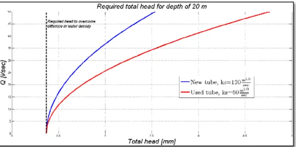
Figure 32: Device capacity for 20 m of water column for different heads and material conditions. ... 51
Figure 33: Device capacity for 50 m of water column for different heads and material conditions. ... 52
Figure 34: Components of OXYFLUX model. ... 54
Figure 35: Details of the floater, all lengths are in mm. ... 55
Figure 36: Details of the tube and of the support for the DOP transducer, all lengths are in mm. ... 56
Figure 37: Vertical velocity profile for H=18.00 mm – T=0.75 sec. and h=400.00 mm. 57 Figure 38: Details of stabilizing ring, all lengths in mm. ... 58
Figure 39: Total buoyancy force vs floater submergence. ... 59
Figure 40: Final design of the tested physical model. ... 60
Figure 41: OXYFLUX physical models. ... 61
Figure 42: Realization of the rigid tube at the Hydraulic Laboratory of University of Bologna.. ... 63
Figure 43: The mechanism used to weld nylon layer. ... 63
xvi
Figure 45: Schematic representation of the two values of crest freeboard (left) and
particular of the physical model (right). ... 65
Figure 46: Test set-up, values in meters. Longitudinal (top) and horizontal (bottom) sections. ... 65
Figure 47: Example of reflection analysis. ... 66
Figure 48: Ratio between the target wave height (Ht) and the incident wave height (Hm_i) ... 68
Figure 49: Reflection coefficients (Hr/Hm_i) ... 68
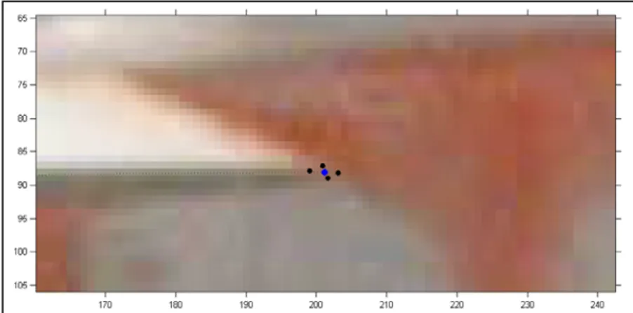
Figure 50: Identification of mean value for the extremes of the floater (mean value blue dot single optical detection black dots) and for water surface position (blue circle). ... 71
Figure 51: Identification of mean values for the extremes of the floater (mean value blue dot, single optical detection black dots) and for water surface position (blue circle). ... 71
Figure 52: Sequence of analyzed frames, [84]. ... 72
Figure 53: Time series measured example ... 72
Figure 54: Time series measured example ... 73
Figure 55: Rigid device moored with chains: wave state C (a), wave state T (b), wave state O (c), wave state E (d) , (measurements are in mm). ... 74
Figure 56: Flexible device moored with chains: wave state C (a), wave state T (b), wave state O (c),wave state E (d), (measurements are in mm). ... 75
Figure 57: Energy spectrum for heave motion, wave state O. Rigid (a), Flexible (b). ... 76
Figure 58: Manual identification of the region of interest (left), zoom on the selected area (right). ... 77
xvii
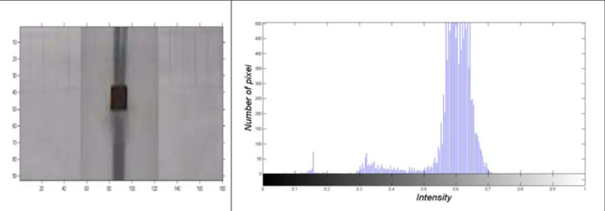
Figure 59: Zoom on selected area of interest before intensity adjustment (left) and its
intensity histogram (right). ... 78
Figure 60: Zoom on selected area of interest after intensity adjustment (left) and its intensity histogram (right). ... 79
Figure 61: Original image (left), complement (right). ... 79
Figure 62: Comparison of the effects of morphological opening (left) and closing (right), with different structuring element, (disk length 7 (1), square length 2 (2), square length 5 (3), square length 8 (4), square length 10 (5), square length 12 (6), square length 13 (7), square length 14 (8)) ... 81
Figure 63: Sequence of the last two steps of the algorithm: conversion of the image in binary and identification of the center of mass of the marker. ... 82
Figure 64: Time response of a freely floating damped heaving unmoored ... 83
Figure 65: alm water test results: unmoored (a), rigid device moored (chains and cables) (b), flexible device moored (chains and cables) (c) ... 85
Figure 66: Comparison of the damping coefficients, peaks envelope ... 85
Figure 67: Facilities at Davidson Laboratory ... 87
Figure 68: Displacements measuring method at Davidson Laboratory ... 88
Figure 69: Experimental RAO for rigid device with no mooring system ... 89
Figure 70: Experimental Response Amplitude Operator (RAO) for rigid device moored with cables; dotted lines indicate standard deviation. They appear only in correspondence to some period, since different wave heights have been tested only for selected wave periods. ... 89
Figure 71: Example of measured time series, Wave n°12 ... 90
xviii
Figure 73: Eddy formation at the stabilizing ring from numerical model. ... 91
Figure 74: Example of measured time series, Wave n°2 ... 92
Figure 75: Experimental Response Amplitude Operator (RAO) for rigid device moored with chains; dotted lines indicate standard deviation. They appear only in correspondence to some period, since different wave heights have been tested only for selected wave periods. ... 92
Figure 76: Comparison between experimental Response Amplitude Operator (RAO) for the rigid device; dotted lines indicate standard deviation. They appear only in correspondence to some points since multiple wave heights have been tested only for selected wave periods. ... 93
Figure 77: Example of measured time series and relative spectral analysis for chains moored device; the non linear behavior of the device is highlighted for wave n° 14 in heave mode. ... 94
Figure 78: Submergence of the floater during wave cycle (%) vs wave period. ... 95
Figure 79: Water particles velocity according linear wave theory for wave state 34 ... 98
Figure 80: Velocity values time series, wave n° 9. ... 100
Figure 81: Velocity values time series, wave n° 9. ... 102
Figure 82: OXYFLUX during a physical test, only the probe and floater are visible (left), cad view of a section of the device with DOP (right). ... 104
Figure 83: Problems relative to the measurements with the flexible structure (right), rigid structure (left)... 105
Figure 84: Vertical water velocity vs. incident wave height, (positive values represent downward water velocities), device moored with cables. ... 106
xix
Figure 85: Vertical water velocity vs. wave steepness, (positive values represent
downward water velocities), device moored with cables. ... 107
Figure 86: Vertical water velocity vs. average submergence level during the wave cycle, (positive values represent downward water velocities), device moored with cables. .... 107
Figure 87: Vertical water velocity vs. incident wave height, (positive values represent downward water velocities), device moored with chains. ... 108
Figure 88: Vertical water velocity vs. wave steepness, (positive values represent downward water velocities), device moored with chains. ... 108
Figure 89: Vertical water velocity vs. medium submergence level during the wave cycle, (positive values represent downward water velocities), device moored with chains. .... 109
Figure 90: Comparison of water velocity results and fitting for the two mooring systems. ... 110
Figure 91: Monitoring of local Courant Number at the surface. ... 122
Figure 92: Geometry input used for the simulations and location of the center of gravity. ... 126
Figure 93: Residual for all solver quantities . ... 129
Figure 94: Domain and boundary conditions... 130
Figure 95: Generated interface at the top of the floater. ... 131
Figure 96: Section view of the domain. ... 131
Figure 97: Section view of the volumetric mesh. ... 133
Figure 98: Section view of the volumetric mesh, thinner mesh layer between the free surface. ... 134
xx
Figure 100:Problem due to the mesh rotation. ... 135
Figure 101: Wave, Heave, Water flow and cumulative pumped volumes for O1. ... 136
Figure 102: Spectral analysis for O1. ... 137
Figure 103: Wave, Heave, Water flow and cumulative pumped volumes for O2. ... 137
Figure 104: Spectral analysis for O2. ... 138
Figure 105: Wave, Heave, Water flow and cumulative pumped volumes for O3. ... 138
Figure 106: Spectral analysis for O3. ... 139
Figure 107: Wave, Heave, Water flow and cumulative pumped volumes for O4. ... 139
Figure 108: Spectral analysis for O4. ... 140
Figure 109: Schematic representation of the region used to discretized the domain. ... 141
Figure 110: Screenshots of the used overset mesh. Representation of the cell type used in the coupling of the two regions, (blue inactive cells , green donor, red intermediate cell layer used by the hole cutting process). ... 142
Figure 111: Domain and boundary conditions... 144
Figure 112: Generated interface at the top of the floater. ... 145
Figure 113: a) Section view x-z, b) section view y-z, c) 3D view of the overset mesh. . 145
Figure 114: Effects of the VOF Wave damping on the free surface and on the water vertical velocity. ... 147
Figure 115: Section views of the overset mesh. ... 148
Figure 116: Thicker zone around the overset region, and boundary layer. ... 149
xxi
Figure 118: Volumetric controls used to describe water surface (UPPER, VB1, VB2, VO ), and to ensure the same grid size in the overlapping region. ... 151
Figure 119: Effects of grid resolution on heave response, red dot is the value used for the simulations ... 152
Figure 120: Effects of sidewall distance on heave response, red diamond is the value used for the simulations... 153
Figure 121: Effects of grid resolution on computed time, red dot is the value used for the simulations ... 153
Figure 122: Effects of wave length discretization on heave response, red dot is the value used for the simulations ... 153
Figure 123: Effects of wave height discretization on heave response, red dot is the value used for the simulations ... 153
Figure 124: Calm water tests from STAR-CCM+ and experimental measurement. ... 155
Figure 125: Heave response of the device, water flow inside the tube and cumulative pumped volume for WAVE 1. ... 156
Figure 126: Heave response of the device, water flow inside the tube and cumulative pumped volume for WAVE 38. ... 157
Figure 127: Heave response of the device, water flow inside the tube and cumulative pumped volume for WAVE 39. ... 157
Figure 128: Heave response of the device, water flow inside the tube and cumulative pumped volume for WAVE 44. ... 157
Figure 129: Heave response of the device, water flow inside the tube and cumulative pumped volume for WAVE C. ... 158
xxii
Figure 130: Heave response of the device, water flow inside the tube and cumulative pumped volume for WAVE T... 158
Figure 131: OXYFLUX’s heave response ... 159
Figure 132: Comparison of experimental and numerical heave response. ... 160
Figure 133: Images sequence of wave crest meeting the floater. ... 162
Figure 134: OXYFLUX’s mean pumped flow. ... 163
Figure 135: Comparison of experimental and numerical mean downward flux. ... 164
Figure 136: Example of spillway designed according Lazzari’s profile, [131] ... 166
Figure 137: Spillway during common operation time, [131] ... 166
Figure 138: Components of Geometry 2 used in numerical model. ... 167
Figure 139: Reference system used to define Lazzari’s profile. ... 168
Figure 140: Details of the floater, all lengths are in m. ... 169
Figure 141: Trend of the buoyancy force for both geometries, the weight has been chosen in order to have the same buoyancy reserve force for both geometries. ... 171
Figure 142: Details of the Geometry 2. ... 172
Figure 143: 3D view of the overset mesh used to simulate Geometry 2. ... 173
Figure 144: OXYFLUX’s response in heave for Geometry 2. ... 175
Figure 145: OXYFLUX’s mean pumped flow for Geometry 2. ... 175
Figure 146: Comparison of water velocity results and fitting for both the mooring systems used... 178
xxiii
Figure 148: Comparison of the mean pumped water flow for Geometry 1 and Geometry
1
CHAPTER I: Introduction
A common worldwide problem: eutrophication and hypoxia
“No other environmental variable of such importance to estuarine and coastal ecosystems around the world has changed so drastically, in such a short period of time, as dissolved oxygen”, [1].
Diaz started his work “Overview of Hypoxia around the World” with the above sentence, testifying how the problem of eutrophication of coastal zones is current and global for present society. The term eutrophication refers to an excessive enrichment of water by nutrients and its associated adverse biological effects,[2]. Cultural eutrophication, which results from human activity, may negatively affect marine ecosystems, increasing the occurrence of massive benthos and fish mortality, loss of diversity, poisoning episodes which can also cause human illness, and mucilage production [3], [4], [5] Eutrophication produces an excess of organic matter that fuels the development of hypoxia and anoxia when combined with water column stratification. Many ecosystems have reported some type of monotonic decline in dissolved oxygen levels through time with a strong correlation between human activities and a decline in declining dissolved oxygen.
Within the past 50 years eutrophication; the over enrichment of water by nutrients such as nitrogen and phosphorus, has emerged as one of the leading causes of water quality impairment. Selman identifies over 415 areas worldwide that are experiencing symptoms of eutrophication, highlighting the global scale of the problem. Recent coastal surveys of the United States and Europe have found that a staggering 78 % of the assessed continental U.S. coastal areas and approximately 65 % of Europe’s Atlantic coasts show symptoms of eutrophication,[6], [7]. In other regions, the lack of reliable data hinders the assessment of coastal eutrophication. Nevertheless, trends in agricultural practices,
2 energy use, and population growth indicate that coastal eutrophication will be an ever-growing problem, [8].
Because of their geomorphology and circulation patterns, some marine systems have a greater tendency to develop hypoxic conditions. The basic features that make a system prone to hypoxia are low physical energy (tidal, currents, or wind) and large freshwater inputs. These features combine to form stratified or stable water masses near the bottom that become hypoxic when they are isolated from reoxygenation with surface waters. Better mixed or flushed systems do not have a tendency towards hypoxia.
What is the hypoxia
Oxygen is necessary to sustain the life of all fishes and invertebrates. In aquatic environments, oxygen from the atmosphere or from phytoplankton dissolves in the water and allows all animals to breathe, including those that swim or move about the sea bottom and those that have a sedentary life. Once dissolved into surface water, the normal condition for dissolved oxygen is to be mixed down into bottom layer waters. When the supply of oxygen to the bottom is cut off or the consumption rate exceeds resupply, oxygen concentration declines beyond the point that can sustain the life of most animals. This condition of low dissolved oxygen is known as hypoxia. The point at which various animals suffocate varies, but generally effects start to appear when oxygen concentration drops below 2 mg/l, [1]. For sea water, this is only about 18 % of air saturation. As a point of reference, air concentration is about 280 mg/l. Anoxia is the complete absence of oxygen. The two principal factors that lead to the development of hypoxia, are decreased water exchange between bottom water and oxygen-rich surface water, and decomposition of organic matter in the bottom water, which reduces oxygen levels. Both conditions must occur for hypoxia to develop and persist.
3
Consequence of the eutrophication
The rise in eutrophic and hypoxic events has been primarily attributed to the rapid increase in intensive agricultural practices, industrial activities and population growth, which together have increased nitrogen and phosphorus flows into the environment. Human activities have resulted in nearly doubling nitrogen and tripling phosphorus flows into the environment compared to natural values, [9]. By comparison, human activities have increased atmospheric concentrations of carbon dioxide, the gas primarily responsible for global warming, by approximately 32 % since the onset of the industrial age, [10].
Before nutrients and nitrogen in particular, are delivered to coastal ecosystems they pass through a variety of terrestrial and freshwater ecosystems, causing other environmental problems such as freshwater quality impairments, acid rain, the formation of greenhouse gases , significant impacts on food webs, and loss of biodiversity, [11].
Once nutrients reach coastal systems, they can trigger a number of responses within the ecosystem. The initial impact of the increase in nutrients is the excessive growth of phytoplankton, microalgae and macroalgae. This, in turn, can lead to other impacts such as:
loss of subaquatic vegetation such as excessive phytoplankton, microalgae, and macroalgae growth which reduces light penetration;
a change in species composition and biomass of the benthic (bottom-dwelling) aquatic community, eventually leading to a reduced diversity of species and the dominance of gelatinous organisms such as jellyfish;
coral reef damage as increased nutrient levels promote algae growth over coral larvae. Coral growth is inhibited because algae outcompete coral larvae for available surfaces to grow on;
4 shifts in the composition of phytoplankton species, creating favorable conditions for
the development of nuisance, toxic, or otherwise harmful algal blooms;
low dissolved oxygen and formation of hypoxic or “dead” zones (oxygen-depleted waters), which in turn can lead to the collapse of the ecosystem.
It is known that eutrophication diminishes the ability of coastal ecosystems to provide valuable ecosystem services such as tourism, recreation, the provision of fish and shellfish for local communities, sportfishing, and commercial fisheries. Furthermore, eutrophication can lead to reductions in local and regional biodiversity.
Currently nearly half of the world’s population lives within 60 kilometers from coastal areas, with many communities relying directly on coastal ecosystems for their livelihoods, [12] This means that a significant portion of the world’s population is vulnerable to the effects of eutrophication in their local coastal ecosystems.
Harmful Algal Blooms and Hypoxia.
Two of the most acute and commonly recognized symptoms of eutrophication are harmful algal blooms and hypoxia. Harmful algal blooms can cause the killing of fish, human illness through shellfish poisoning, and the death of marine mammals and shore birds. Harmful algal blooms are often referred to as “red tides” or “brown tides” because of the appearance of the water when these blooms occur. One red tide event, which occurred near Hong Kong in 1998, wiped out 90 percent of the entire stock of Hong Kong’s fish farms and resulted in an estimated economic loss of $40 million USD, [13]. Hypoxia, which is considered to be the most severe symptom of eutrophication, has escalated dramatically over the past 50 years, increasing from about 10 documented cases
5 in 1960 to at least 169 in 20071,[14]. Hypoxia occurs when algae and other organisms die, sink to the bottom, and are then decomposed by bacteria using the available dissolved oxygen. Salinity and temperature differences between surface and subsurface waters lead to stratification, limiting oxygen replenishment from surface waters and creating conditions that can lead to the formation of a hypoxic or “dead” zone, [15].
Nutrients, eutrophication and hypoxia: an overview on the connections
The primary factor driving coastal eutrophication is an imbalance in the nitrogen cycle that can be directly linked to increased population, due either to urbanization in coastal areas or along rivers or to the development of agricultural activities. In many areas hypoxia follows from eutrophication, which results from the underlying nutrient problem. An examination of the distribution of hypoxic zones around the world showed that they were closely associated with developed watersheds or highly densely populated coastal areas that deliver large quantities of nutrients, the most important of which is nitrogen, to coastal seas,[16]. Agriculture and industry are regarded as the principal generators of nitrogen, even if, in the end increased population and rising living standards drive the need for industry and agriculture to produce. Atmospheric sources of nitrogen are also recognized as a significant contributor of nutrients in coastal areas, [17]. Nitrogen from fossil fuel combustion and volatilization from fertilizers and manure is released into the atmosphere and redeposited on land and in water by wind, snow, and rain.
1
6 The degenerative scenario linking nutrient additions to the formation of hypoxia via eutrophication, following an initial positive effect on fisheries, can be described as follow:
Excess nutrients lead to increased primary production, which represents new organic matter that is added to the ecosystem. Since shallow estuarine and coastal systems tend to be tightly coupled (benthic-pelagic coupling), much of this organic matter reaches the bottom. This increased primary productivity may also lead to increased fishery production, [18] At a certain point, however, the ecosystem's ability to maintain a balance in processing organic matter is exceeded. If physical dynamics permit stratification, hypoxic conditions develop. Initially, increased fishery production may offset any detrimental effects of hypoxia but, as eutrophication increases and hypoxia expands in duration and area, the fishery production base is affected and declines. The increasing input of anthropogenic nutrients to many coastal areas over the last several decades has been suggested as being the main contributor to the most recently declining trends in bottom water oxygen concentrations around the world. Many studies have demonstrated a correlation through time between population growth, increased nutrient discharges, increased primary production in coastal areas and increased occurrence of hypoxia and anoxia; an example might be the decline in oxygen concentration in the Gulf of Trieste in the last 25 years, [1]. . The direct connection between land and sea is best exemplified by the relationship between estuarine and coastal fishery production and land-derived nutrients. The most productive fishery zones around the world are always associated with significant inputs of either land (runoff) or deep oceanic (upwelling) derived nutrients. The basic nutrients carried by land runoff and oceanic upwelling are the essential elements that fuel primary production and that, through marine food webs, feed the species of economic importance. Problems begin when the nutrients entering the system exceed the capacity of the food chain to assimilate them. At first, increased nutrients lead to increased fishery production but, as organic matter production increases, changes occur in the food web leading to different endpoints. These changes are very predictable
7 and have been recognized in many marine ecosystems, Figure 1. Basically, a hypoxic zone is the secondary manifestation of the larger problem of excess nutrients, which leads to increased production of organic matter or eutrophication,[19]. When eutrophication combines with water column stratification, hypoxia results.
Figure 1: Comparative evaluation of fishery response to nutrients,[18].
Locations of global eutrophic and hypoxic areas
The latest results of a survey on eutrophic and hypoxic zones date back to 2008, when Selman et al. found 415 systems which presented problems related to eutrophication. Of these, 169 are documented hypoxic areas, 233 are areas of concern, and 13 are systems in
8 recovery. The advances in identifying and reporting eutrophic conditions will rapidly lead to the growth of the number of known areas. The first comprehensive list of hypoxic zones was compiled by Diaz and Rosenberg in 1995 [20] and identified 44 documented hypoxic areas, nearly one quarter of the hypoxic areas identified by Selman et al. twelve years later, [14]. The list of hypoxic areas assembled by Diaz was compiled from scientific literature and identified the majority of the documented hypoxic areas. However, the list did not include areas with suspected but not documented hypoxic events or systems that suffer from other impacts of eutrophication such as nuisance or harmful algal blooms, loss of subaquatic vegetation and changes in the structure of the benthic aquatic community. The supplementary list of hypoxic zones, shown in Figure 2, takes into account systems experiencing any symptoms of eutrophication, including but not limited to anoxia. The new zones are divided into:
documented hypoxic areas: areas with scientific evidence that hypoxia was caused, at
least in part, by nutrient overenrichment;
areas of concern: systems that exhibit effects of eutrophication, such as elevated
nutrient levels, elevated chlorophyll levels, harmful algal blooms, changes in the benthic community, damage to coral reefs and fish kills. These systems are impaired by nutrients and are possibly at risk of developing hypoxia;
systems in recovery: areas that once exhibited low dissolved oxygen levels and
9
Figure 2: World hypoxic and eutrophic coastal areas, [8].
Wave Energy Converter, Strengths and weaknesses
History of the Ocean Wave Energy Converters
Energy from ocean waves is the most conspicuous form of ocean energy, possibly because of the often spectacular destructive effects of the waves. The waves are produced by wind action and are therefore an indirect form of solar energy, [21]. The opportunity of converting wave energy into usable energy has inspired numerous inventors: more than one thousand patents had been registered by 1980,[22] and the number has increased markedly since then. The earliest patent was filed in France in 1799 by a father and a son named Girard,[23].
Yoshio Masuda may be regarded as the father of modern wave energy technology, with his studies in Japan dating from the 1940s. He developed a navigation buoy powered by wave energy, equipped with an air turbine, which was in fact what was later named a
10 (floating) oscillating water column (OWC). These buoys have been commercialized in Japan since 1965, [24]. In 1976 Masuda promoted the construction of a much larger device: a barge, named Kaimei, which was used as a floating testing platform housing several OWCs equipped with different types of air turbines, [25]. Probably because this was done at an early stage, when the theoretical knowledge on wave energy absorption was at its beginning, the power output levels achieved in the Kaimei testing program were not a great success. Masuda realized that converting wave energy to pneumatic energy with the Kaimei project was quite unsatisfactory and conceived a different geometry for a floating OWC: the Backward Bent Duct Buoy (BBDB). In the BBDB, the OWC duct is bent backwards from the incident wave direction, (Figure 3), which was found to be advantageous when compared to the frontward facing duct version,[26]. In this way, the length of the water column could be made sufficiently large enough for resonance to be achieved, while keeping the draught of the floating structure within acceptable limits. The BBDB converter was studied (including model testing) in several countries (Japan, China, Denmark, Korea, Ireland) and was used to power about one thousand navigation buoys in Japan and China,[27], [28].
In 1974, a paper published by Stephen Salter,[29] became a landmark and brought wave energy to the attention of the international scientific community. In 1975 the British Government started an important research and development program in wave energy,[21], followed shortly afterwards by the Norwegian Government. In Norway the activity resulted in the construction of two full-sized shoreline prototypes near Bergen in 1985. In the following years, up until the early 1990’s, the activity in Europe remained mainly at an academic level; the most visible achievement being a small OWC shoreline prototype deployed on the island of Islay, Scotland,[30]. At about the same time, two OWC prototypes were constructed in Asia: a converter integrated into a breakwater at the port of Sakata, Japan,[31]and a bottom-standing plant at Trivandrum, India,[32].
In 1991 the situation in Europe was dramatically changed by the decision made by the European Commission of including wave energy in their R&D program on renewable
11 energies. The first projects started in 1992. Since then, about thirty projects on wave energy were funded by the European Commission involving a large number of teams in Europe,[21]. In the last few years, interest in wave energy has been growing in northern America, involving national and regional administrations, research institutes and companies, and giving rise to frequent meetings and conferences on ocean energy, [33], [34].
Figure 3: Schematic representation of Backward Bent Duct Buoy, [21].
Strengths and weaknesses of the Wave Energy Converter
The development of wave energy converter devices is characterized by numerous inventions. Since the first patent on wave energy,[23], a great number of ideas to harness the energy of waves has been conceived; however, only few of them have succeeded in being tested in the sea.
Nowadays developing wave energy converters is no longer a privilege of virtuous and wealthy Nations. Even if it does not still represent a safe business, obtaining energy from waves allows for the creation of new jobs and the production of clean energy characterized by a low environmental footprint. Wave energy is a concentrated and
12 readily available energy source, unlike fossil fuels which, in some places in the world, are running out just as quickly as people can discover them. Unlike ethanol, a corn product, wave energy is not limited by seasons and it does not need any kind of intervention from man,[35]. It is close to densely populated areas and is well distributed around the globe and it has a very low visual impact. Moreover, wave energy can be predicted with good accuracy and is more constant than wind energy, [36].
Nevertheless, the road ahead for the realization of efficient wave energy converters is beset with difficulties, particularly related to testing in real seas, due to the characteristics of ocean waves and to the related costs. Contrary to many other WECs, the system has to be tested in real seas on a certain prototype scale. Sea trials are generally more complicated and expensive than laboratory testing [37]. The deployment also requires suitable weather windows and specific vessels. Above all, the prototype has to be designed to survive extreme events and to operate in harsh environments, despite being a test plant. The extreme conditions at the deployment location, although being infrequent, dictate the structural design of the WECs and mooring systems, which are also directly linked to the overall investment. All these factors strongly affect project costs. Many failures in this sector, (like mooring breakages and WECs getting stranded before an audience) are retained and emphasized by the public and other stakeholders. On the other hand, one of the biggest success stories of the sector must be recalled. There are about three hundred OWCs navigational buoys functioning around the world in places where battery changing, lighting a 60 W bulb and driving a flashing unit, as designed by Commander Yoshio Masuda, is inconvenient [34].
Concerning the environmental impacts, the problems due to WECs are probably few, and mostly unknown. Some stakeholders' concerns regard the negative impacts on fisheries or marine mammal migration, with marine life risking getting entangled in cables. Apart from wildlife conservation and site specific environmental issues other recommendations for suitable sites for wave energy converters include: avoidance of shipping lanes, avoidance of areas of military importance, and marine archaeological sites. Other
13 potential conflicts include areas intended for mining or for the dredging of sand and gravel. Further restrictions on the placement of WECs comes from existing pipelines and cables, although most likely on a smaller scale. Already existing offshore activities limit future establishments, including offshore wind power parks, oil and gas fields,[38]. Wave power converters are less likely to interfere with recreational activities such as leisure boats, since parks may be placed far off the coast, [36]. Although the techniques are generally not very well developed yet, it is likely that wave power will become at least as important as wind and hydropower are today,[39].
14
CHAPTER II: Literature Survey
Adriatic Sea Conditions
The Adriatic Sea is an elongated basin, with its major axis oriented in a northwest - southeast direction, located in the central Mediterranean, between the Italian peninsula and the Balkans.
Figure 4: Adriatic Sea coastline an topography, [40].
Its northern section is very shallow and gently sloping, with an average bottom depth of about 35 m. Middle Adriatic average depth is 140 m, with the two Pomo Depressions reaching 260 m. The southern section is characterized by a wide depression more than 1200 m deep. The water exchange with the Mediterranean Sea takes place through the
15 Otranto Channel, whose sill is 800 m deep. The eastern coast is characterized by rocky shores and cliffs, whereas the western coast is flat and mostly sandy. A large number of rivers discharge into the basin, with significant influence on the circulation, particularly relevant being the Po River in the northern basin, and the ensemble of the Albanian rivers in the southern basin,[40].
The structure and the seasonal variability of the Adriatic general circulation is synthesized in Fig. 5. At the surface the winter general circulation is composed only of the Northern and Southern Adriatic current (NAd and SAd) segments and the flow field is very different from all other seasons. The general circulation is dominated by temperature and salinity compensation effects. It can be speculated that the barotropic, wind-induced transport and circulation is probably a major component of the general circulation during winter. This can also be estimated by looking at the seasonal water mass properties [40], where during winter and throughout the basin vertical temperature and salinity profiles become practically uniform with depth. Spring–Summer surface flow field is characterized by the appearance of western current segments (W-Mad and W-SAd) and the two major cyclonic gyres of the Adriatic circulation. It can be argued that the seasonal vertical stratification in the basin triggers the appearance at the surface of gyres and an intensification of boundary currents, more generally of eddies and jets, probably as a result of baroclinic-barotropic nonlinear instabilities in the basin,[41].
16
Figure 5: Adriatic Sea general circulations,[41].
During summer currents occur on smaller spatial scales and the E-SAd current weakens. Autumn conditions are characterized by the maximum spatial coherence of the general circulation structure. In fact, there are three cyclonic gyres, a continuous western Adriatic boundary current, connected between the three subbasins, and an intense SAd current. As known from [40], this season is characterized by maximum middle levantine intermediate water entrance and spreading from Otranto, a well-defined surface mixed layer and maximum warming of the subsurface layers of the northern Adriatic.
Anoxia in the northern Adriatic
The northern Adriatic is a shallow basin characterized by a cyclonic circulation and by the inputs of many rivers; Po and Adige contribute to the most of the total freshwater input. Anthropogenic nutrient loads coming from rivers flowing into the north-western
17 Adriatic Sea have considerably increased during the late 20th century, especially between 1968 and 1980,[42]. A major fraction of the productivity in surface waters reaches the sea floor [43] and anoxic or near anoxic events frequently occur in bottom waters, especially during late summer and autumn as a consequence of high downward of organic fluxes, microbial decay and thermal stratification,[44], [45], [46]. High concentrations of particulate organic matter are present in the north west Adriatic due to the combined effects of terrestrial suspended matter input and primary productivity, which depends highly upon nutrient load discharged by rivers, [47]. Consequently, massive diatom and dinoflagellate blooms and “red tides” (sometimes associated with toxicity episodes) are well known along the northwestern Adriatic coast,[5]. In the Adriatic basin, a trophic gradient increasing from east to west is present. In the western side of the basin, particulate organic matter (POM) reaches higher concentrations, especially in proximity of the deltas of Adige and Po,[48]. The POM, diffusing through the water column, represents an important source of energy for the benthic system and through the degrading processes contributes to the decrease of oxygen content in the bottom waters. In coastal environments, the flux of settling particles is influenced by river discharge, physical and chemical reactions at the fresh-salt water interface, primary and secondary production and water circulation, [49]. The downward flux of particulate organic matter in the shallow northern Adriatic basin is relevant both for the sinking and recycling of nutrients and for the oxygen consumption at the bottom, which often causes local hypoxia in the coastal belt and occasionally may lead to basin scale hypoxia events, when general circulation and wave intensity are reduced.
Water mass structure: temperature, salinity, dissolved oxygen and stratification of the North Adriatic Sea
The shallow northern Adriatic Sea is characterized by marked seasonal and long-term fluctuations of oceanographic and biological conditions, mainly due to atmospheric
18 forcing, freshwater discharges, variable intrusion of high salinity waters, and a very variable and complex circulation,[50], [51]. Due to intense heat losses Fig.6, at the air– sea interface, the water column of the offshore North Adriatic is well mixed during late autumn and winter.
Figure 6: Monthly mean heat flux at the surface (W/m2), estimations based on 4 different datasets,[40]. Water mass exchange between northern and central Adriatic is at its maximum during this period, characterized by a prevailing cyclonic circulation, and by northward currents in the eastern part and southward currents along the western coast, [51]. During spring dense water generally remains in the bottom layer in northernmost areas and as a vein along the western side of the entire region. During spring and summer, semi-enclosed circulation patterns prevail in the region, and thermal stratification gradually increases and reaches its maximum in August as a result of heat accumulation in the upper layers, [52]. In these conditions freshened surface waters, formed along the western coast, are generally advected eastward to the Istrian coast, so significantly increasing the stratification of the water column.
19 Particular freshwater discharge dynamics in spring and summer, characterized by relevant peaks of short duration, may play an important role for the development of the mucilage phenomenon, particularly in conditions of reduced water dynamics, [4],[53]. This phenomenon is characterized by the formation of macro-aggregates of different shapes and dimensions in the upper water column of the entire northern Adriatic.
Temperature and Salinity
Figure 7, shows the climatological medium profiles for temperature and salinity obtained for the entire Adriatic Sea. In the northern Adriatic the entire water column exhibits an evident seasonal thermal cycle. A well-developed thermocline is present in spring and summer down to 30-m depth, whereas a significant cooling begins close to the surface in autumn when the bottom temperature reaches its maximum value, probably due to increased vertical mixing and intrusion of middle Adriatic waters.
20
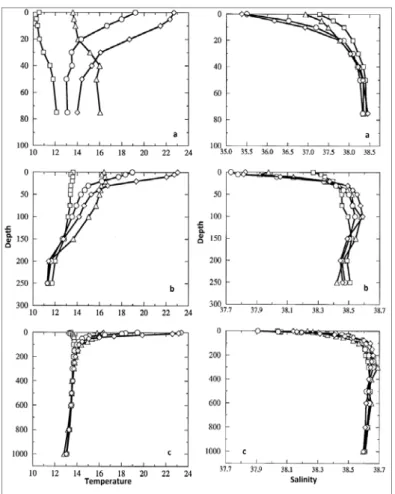
Figure 7: Seasonal climatological profile of Adriatic, a) Northern Adriatic, b) Middle Adriatic, c) Southern Adriatic. The variables represent are Temperature, °C, (left); and Salinity, ppm, (right). Spring , summer
, autumn , winter , [40].
The cooling of the whole water column only occurs in winter; in this season temperature generally increases down to the bottom, but the water column stability is preserved due to an associated increase of salinity at depth. The effects of freshwater input can be clearly seen in spring and summer due to the increased runoff and the increased water column stratification, [41].
Dissolved oxygen
Except for its northern part, the Adriatic Sea is a well-oxygenated basin. The dissolved oxygen profiles show that in the warmer seasons a relatively low concentration layer is present just near the sea surface, due to oxygen equilibration with the atmosphere,[40]. In
21 the northern Adriatic it can be noticed that the average oxygen profiles have a qualitatively different shape of with respect to middle and southern Adriatic conditions. The northern Adriatic can be subdivided in two sub regions, the first corresponding to areas shallower than 50 m, Figure 8a and Figure 8b, and the second corresponding to the remaining part Figure 8c.
Figure 8: Seasonal climatological profile of Adriatic: a) Northern Adriatic shallower or equal to 50 m, b) northern Adriatic deeper than 50 m, c) middle Adriatic, d) southern Adriatic max depth, e) southern Adriatic shallower or equal to 300 m. Dissolved oxygen (ml/l). Spring , summer , autumn , winter
, [40].
The average value of dissolved oxygen in the Adriatic basin is approximately 5.5 ml/l. The parameter wich has been used to describe the variability of the dissolved oxygen is standard deviation (STD). Lowest variability of dissolved oxygen appears near the bottom in autumn (STD equal to 0.1 ml/l) and summer (STD equal to 0.4 ml/l), while the
22 highest STD value occurs at the surface with values of 0.5 - 0.6 ml/l in all seasons except for summer, when the highest STD of 0.9 ml/l is found at a depth of 30 m, [40].
In this chapter an overview on the climatological water mass and dissolved oxygen structure is proposed. The whole Adriatic basin can be divided in three main sectors: northern, the shallowest; middle, the transitional area; southern zone, the deepest and the interface with the Ionian Sea. Each of them is characterized by its own profiles of temperature, salinity and dissolved oxygen level. No differences can be found for the water surface characteristics between the three areas. All of them are sensible to the seasonal climatological cycle, presenting the highest values of temperature during summer and the deepest level of column agitation during winter. At the surface salt balance is largely affected by river runoffs, especially during spring and summer.
Wave climate of North Adriatic
Leder in 1998 [54] was the first to investigate the characteristic wave climate of the northern Adriatic Sea from measured data. His study was aimed to identify the monthly significant wave height through Gumbel distribution fitted on data measured in the offshore part of the northern Adriatic Sea from the platforms Panon and Labin, Figure 9.
23 Monthly extreme values were available for a ten year period (1978–1986 and 1992). The absolute maximum significant wave height measured in those 10 years was 6.58 m recorded during a storm in December 1979. The wave height of 10.2 m was measured during that storm, being the second highest measured wave in the Adriatic Sea. The largest individual wave height recorded so far in the Adriatic Sea reads 10.8 m. The wave was measured in the Northern Adriatic in February 1986 during a storm with a significant wave height of 6.16 m. The theoretical prediction of the most probable extreme significant wave height in 20 and 100 years by [54], reads 7.20 and 8.57 m, respectively, Table 1. It should be mentioned that another study has been conducted,[55], but, since it was based on data collected by observations from merchant ships, which are better suited to the analysis of seagoing ships comparing to the data from the fixed measurement stations,[56],[57] it will not be considered.
Table 1: Average monthly and annual wave power significant wave heights (m), Tr return period (years), [58].
Such values were calculated in order to identify the extreme events, with the aim to develop an helpful tool for people working in activities related with this area of the Adriatic. Hypoxia develops during period of stable stratification, when the waves are not strong enough to break this layer. Thus extreme waves are not indicators for events related to the anoxia, but they can give an idea of the low wave power in the North Adriatic (compared with other extreme wave climates).
24 Vicinanza in [58], used the available data recorded by the Italian Buoy Network (IWN), [59], that is active since July 1998, to characterize wave power around Italian coasts. IWN offshore wave measurements are available for 15 different sites highlighted in Fig. 9, but for the present study only results coming from buoy 15 are relevant. From 1989 up to about 2002, each wave buoy collected 30 minutes of wave measurements every three hours but in presence of wave heights greater than 1.5m the measurements were continuous. From 2002 wave measurements have always been continuous and wave characteristics parameters refer to 30 minutes time intervals.
Figure 10: Location of the IWN buoys, [58].
In [58] Vicinanza identified the average monthly and annual value of offshore wave power for the Adriatic Sea. It can be argue that the Adriatic has the lowest energetic level, with peak of low level of agitation in its northern area. Table 2 shows the entire dataset identified by Vicinanza and, as expected, during summer a generalized trend of low values of monthly averaged value is recognized. Results coming from buoy 15,
25 related to June, July and August, report 1.2, 0.6 and 0.9 kW/m respectively; even buoy 2 shows low wave power for the same period (0.5, 0.7 and 0.7).
Table 2: Average monthly and annual wave power (kw/m), [58].
Monthly and annual values of wave power are good indicators of the global wave climate; Table 2 presents annual wave power values below 2 kw/m only for the buoys along the Adriatic coast and Catania coast.
The northern Adriatic is one of the most delicate environmental in the entire Mediterranean Sea and its dynamic seems to be independent from the middle and southern Adriatic,[40]. However, it shows its influence on the other two regions through the North Adriatic deep water. Its large river runoff brings a great amount of nutrient that, when combined with summer wave climate and strong vertical stratification, produces the ideal environment to develop hypoxia or anoxia. This work focus is to develop a device especially designed for summer wave climate in seas like North Adriatic; the declared aim does not represent a restriction, since the device will be able to work in all the Seas that, always more frequently, exhibit symptoms of eutrophication and hypoxia. Seas characterized by these phenomena show, during hypoxic or anoxic events, a wave climate that presents different steepness and direction but its heights are of the same order of magnitude of the northern Adriatic Sea; between, completely flat sea and 0.40 m.
26
Wave Overtopping
Research on wave overtopping of coastal structures has been the subject of numerous investigations over the past 50 years. Since then overtopping prediction tools for typical sea defense structures have continuously been refined. The term wave overtopping is used here to refer to the process where waves hit a sloped structure, run up the slope and eventually, if the crest level of the slope is lower than the highest run-up level, overtop the structure, Figure 11.
Figure 11: Wave overtopping of the Wave Dragon prototype,[60].
The discharge from wave overtopping is thus defined as overtopping volume (m3) per time (s) and structure width (m). The reason for predicting overtopping of structures is to design better structures to protect human lives and significant structures against the violent force of the surrounding sea. Typically, rubble mound or vertical wall breakwaters have been used for the protection of harbors and dikes and offshore breakwaters have been used for the protection of beaches and land. All these structures are designed to avoid the risk of overtopping or at least to reduce it to a minimum, since overtopping can lead either to functional or structural failure of structures.
27 The research described in this thesis has a slightly different target; in fact it is aimed to use wave energy to pump water from the surface to the bottom with a simple and economical device able to catch even waves characterized by a low level of energy and convert the overtopping discharge into a downward flux. Economical or energetic fields are not concerned in the present study; the only purpose of this work is to improve the quality of deep water.
Wave overtopping studies: present knowledge
A number of different methods are available to predict overtopping of particular structures under given wave conditions and water levels. Each method has its strengths and weaknesses under different circumstances. In theory, analytical methods can be used to relate the driving process and the structure to the response through equations based directly on a knowledge of the physics of the process. It is however extremely rare for the structures, the waves and the overtopping process to all be well-controlled and known so that an analytical method can give reliable predictions. Other methods are based on the use of measured overtopping from model tests and field measurements. They can use the neural network tool trained using a test, [61]. The last method is based on physical modelling and it consists in testing a scale model with correctly scaled wave conditions. Usually, such models may be built in a scale typically ranging between 1:20 to 1:60. Physical models can be used to measure many different aspects of overtopping such as wave-by-wave volumes, overtopping velocities and depths. Past physical investigations on the wave overtopping of marine structures highlighted that the discharge does not depend only on environmental condition such as wave height, wave period and level but also on the geometrical layout and on the material of the structure, [62], [63]. A lot of investigations have been conducted but none of them has been able to describe all the possible situations. The most common and reliable way of investigation is the physical modelling. Such type of investigation aims to identify an empirical relationship between
28 environmental conditions, geometrical layout and material properties of the structure and the overtopping discharge. Several formulas have been produced, since the first study conducted by Owen, [64] in 1980. The research was aimed to investigate the overtopping over a specific classes of coastal frameworks that included impermeable and smooth, rough and straight and bermed sloped structures. In his work Owen determined the first experimental method to quantify the overtopping flow rate. The formula was an exponential equation that gave as a result a dimensionless value of the overtopping discharge and the input was a dimensionless parameter dependent by the free board of the breakwater. Since 1980 ten new equations have been proposed, but all of them were based on the same exponential structure of the Owen’s formula, [65], [66], [67], [68],[69], [70],[71], [72], [73], [62]. In order to clarify the status of the present knowledge Burcharth wrote in 2000 a comprehensive overview on overtopping of coastal structures, [74], where more details on some of the prediction formulae are available. Douglass, in 1986 [75], reviewed and compared a number of methods for estimating irregular wave overtopping discharges. He concluded that overtopping discharges calculated using empirically derived equations can only be considered within a factor of the actual overtopping discharge. The abovementioned methods deal with overtopping of coastal defense structures and so the typical crest freeboards are relatively high and the overtopping discharges low. Under such conditions overtopping discharge depends on relatively few and relatively large overtopping events. That means that the overtopping discharge becomes very sensitive to the stochastic nature of irregular waves. It must be expected that uncertainty in estimating the overtopping discharge are going to be reduced if the crest freeboard is reduced, since more waves are able to overtop the structure. Before Kofoed 2002 [62], all available the studies and researches aimed to estimate the overtopping discharge for a ground-based structures. The advent of floating overtopping wave energy converters required more accurate equations that can take into account how the level of buoyancy affects the water flow over the structure. In his research Kofoed made large series of laboratory tests in order to incorporated some correction factors
29 related to slope angle, crest free board, draft, slope shape and shape of guiding walls into the expression proposed by Van der Meer 1995, [70].
Figure 12: Parameters investigated by Kofoed,[62].
The results of the new equation proposed by Kofoed fitted experimental data very well, R2 (square of the Pearson product moment correlation coefficient) increases from 0.75 (van der Meer’s equation) to 0.97 (Kofoeed’s equation, below).
∙ ∙ ∙ ∙ 0.2 ∙
. ∙ ∙ ∙ ∙ ∙ ( 1 )
Where λα , λdr and λs are defined by Kofoed and γr, γb, γh and γβ are defined by Van der Meer, 1995, [70].
30
Influence of slope angle
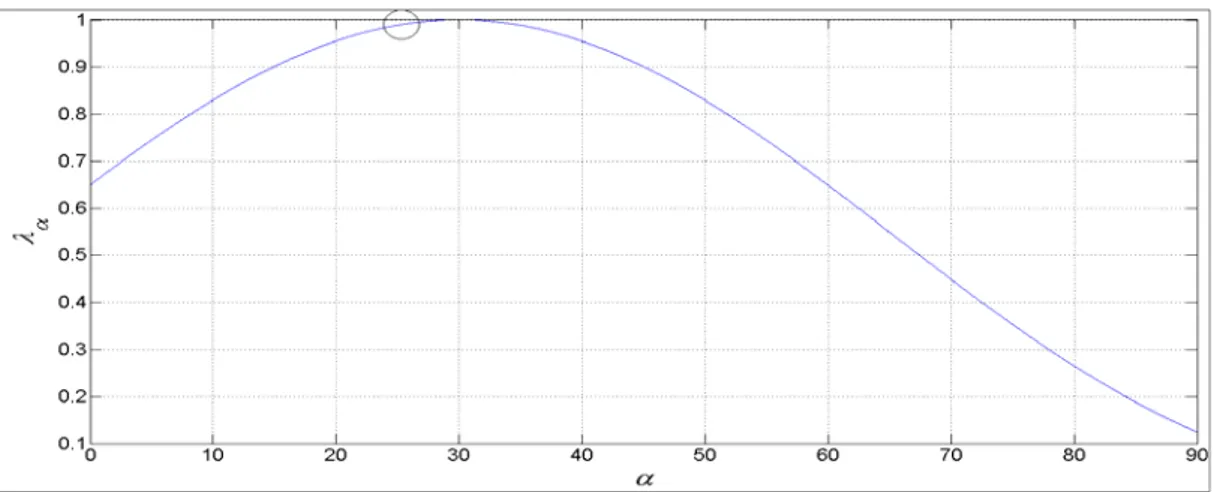
Completed test series by Kofoed, with varying slope angle shows that the average overtopping discharge is slightly dependent an α. Introduced corrector factor λα was identified in order to take into account this dependency, its equation is:
∙ ( 2 )
where αm is the optimal slope angle, equal to 30° and β is a coefficient equal to 3, both values are identified by best fit. Equation 2 is formulated so that the result is for optimal slope angle and it decreases when difference between optimal and actual slope angle increases. The correction factor λα for the device here investigated is equal to 0.989, with a slope angle of 25.4°, see Appendix A for the calculus.
Figure 13: λα as a function of the slope angle. Value for tested shape in present work is black circle.
Influence of draft
Conducted test series by Kofoed with varying draft shows results strongly affected by this parameter. In order to take into account this dependency the coefficient proposed is:
31
1 ∙ ∙ ∙ ∙ ∙ ∙ ∙∙ ∙∙ ∙
( 3 )
where kp is the wave number based on Lp and k is a coefficient controlling the degree of influence of the limited draft. k is equal to 0.4 by nest fit. The expression taking the dependency of the draft into account is based on the ratio between the time averaged amount of energy flux integrated from the draft up to the surface Ef,dr and the time averaged amount of energy flux integrated from the seabed up to the surface Ef,d.
, , ∙ ∙ 1 ∙ ∙ ∙ ∙ ∙ ∙ ∙ ∙ ∙ ∙ ( 4 )
Figure 14: Ratio described by equation 4 as a function of the relative draft, [62].
To derive equation 3 linear wave theory has been used; this implies a limitation that leads to a not exact description of the overtopping phenomena.
The correction factor λdr for the device here investigated is equal to 0.8101 for a draft equal to 0.37 m and a freeboard crest of 0.11 m.
32
Figure 15: λdr as a function of the relative draft. Two freeboard levels for wave state T (H=0.48 m and
T=2.88 sec).
Influence of dimensionless freeboard parameter (R)
Kofoed identified that for values of dimensionless freeboard (R) larger than 0.75 the equation given in [70], fit the data very well, but when the R decries from 0.75 to 0 some discrepancies appear between the predicted values and the observed values. In order to increase the degree of description of the phenomena parameter proposed by Van der Meer was modified as follow:
0.4 ∙ sin ∙ ∙ 0.6 0.75
1 0.75
![Figure 14: Ratio described by equation 4 as a function of the relative draft, [62].](https://thumb-eu.123doks.com/thumbv2/123dokorg/8162040.126709/54.892.160.750.428.809/figure-ratio-described-equation-function-relative-draft.webp)
![Figure 17: q [m 3 /m/sec] as a function of dimensionless freeboard parameter (R c /H s )](https://thumb-eu.123doks.com/thumbv2/123dokorg/8162040.126709/57.892.159.797.159.466/figure-sec-function-dimensionless-freeboard-parameter-r-h.webp)
![Figure 19: The SSG pilot plant in the Island of Kvitsøy, Norge, [90].](https://thumb-eu.123doks.com/thumbv2/123dokorg/8162040.126709/61.892.259.687.158.436/figure-ssg-pilot-plant-island-kvitsøy-norge.webp)