APPENDIX A.
CODES USED WITHIN THE RESEARCH
A.1
The Monte Carlo based neutron transport code MCNP5
The name Monte Carlo is used to identify a class of mathematical methods. Historically, this name was given by the scientists working on the development of nuclear weapons in Los Alamos in the 1940s. In nuclear analysis the Monte Carlo estimates the system characteristics through multiple computer simulations of the behavior of individual particles in the system. This approach is completely different from the deterministic methods. In the latter case the system to be analyzed is divided in several sub-region and the neutron balance equation is solved in those smaller units. Then, the neutron balance equation over the small units is derived and subsequently solved. For the neutronic analysis the deterministic and Monte Carlo methods are the main methodologies employed.
The use of Monte Carlo is much appreciated to investigate phenomena requiring 3D representation with high level of spatial and energetic detail. In this research the Monte Carlo code MCNP5 was used [17]. This code was developed at Los Alamos National Laboratory (LANL), USA.
MCNP5 is a general-purpose, continuous-energy, generalized-geometry, time-dependent, coupled neutron/photon/electron Monte Carlo transport code. It can be used in several transport modes: neutron only, photon only, electron only, combined neutron/photon transport where the photons are produced by neutron interactions, neutron/photon/electron, photon/electron, or electron/photon. The neutron energy regime is from 10-11 MeV to 20 MeV for all isotopes and up to 150 MeV for some isotopes, the photon energy regime is from 1 keV to 100 GeV, and the electron energy regime is from 1 KeV to 1 GeV. Detailed information about MCNP5 code and methodologies can be found in [17]. Hereafter, the most important features of MCNP5 used in this research are reported.
A.1.1.
General scheme of a Monte Carlo method
The Monte Carlo method simulates the neutron history starting from its bird. Each event in its life is selected using pseudo-random variables [42]. Several kind of events can undergo a neutron, e.g. absorption, scattering, leakage etc.
The whole set of events through the neutron life is called neutron history. A quantity of interest (e.g. neutron flux) is obtained simulating a large number of histories and the result is calculated by averaging the quantity of interest over all number of simulations. In addition, the statistical error (or the variance) can be determined along with the average result. A sketch of a Monte Carlo neutron history simulation scheme is reported in Figure 141.
A.1.2.
Estimation of the multiplication factor
The effective multiplication factor (keff) is a quantity of interest in the neutronic
analysis. In a Monte Carlo simulation the neutron histories are divided in many cycles. A user-defined number of histories are simulated in each cycle, then, at the end of the cycle, the keff is calculated. Usually, an initial number of histories are
used for the spatial convergence of the source distribution, hence, such histories can be discarded. Thus, The final keff is the statistical average of the keff from all cycles except the initial number of discarded cycles.
In the MCNP5 code, keff in each cycle is calculated by three methods and the final
keff of the cycle is simply the combined result from each method using observed
correlations to provide the optimum estimate of keff and its standard deviation. The three methods are collision estimator, absorption estimator and track length estimator. The expression for each estimator is given in the following equations:
Absorption estimator Collision estimator Track length estimator With the following meaning of symbols:
• i: ith collision where fission is possible
• k: kth nuclide of the material involved in the ith collision • σT: Microscopic total cross section
• σc: Microscopic capture cross section • σf: Microscopic fission cross section • ρ: The atomic density in the cell • N: Nominal source size for cycle • Wi: Weight of particle entering collision • fk: Atomic fraction for nuclide k
• νk: Average number of neutrons produced per fission
In a Monte Carlo calculation each results is given together its standard deviations. The average results associated with their standard deviation essentially form confidence intervals based on the Central Limit Theorem. In general, the average result plus/minus one standard deviation provides 68% confidence interval while the average result plus/minus two and three standard deviations provides 95% and 99% confidence intervals respectively.
A.1.3.
Evaluation of neutron flux
The quantities of interest in a Monte Carlo simulation are calculated during simulation of the neutron histories. The MCNP5 code provides the user with a
interest will be focused mainly in the calculation of the neutron flux. The average neutron flux in a region can be defined as [17]
Where, N(r,E,t) is the population of neutron in region of volume V, then integration is done over an energy range E, volume V and the differential unit of track length ds. The MCNP5 code utilizes the track length estimator to calculate the neutron flux. The quantity N(r,E,t)ds is evaluated as a track length density. Hence, the average flux can be estimated by summing track lengths Tl weighted with the particle weight W. MCNP5 estimates ΦV by summing WTl/V for all particle tracks in the cell.
This tally can be used to calculate for example the number of fissions, the number of absorptions or any product of the flux times the approximately 100 standard ENDF reactions. Then, Several options can be selected by the user, e.g. the flux can be calculated over a user defined energy bins.
The track length estimator is generally quite reliable because there are frequently many tracks in a cell (compared to the number of collisions), leading to many contributions to this tally.
MCNP tallies are normalized to be per starting particle and are printed in the output accompanied by a second number R, which is the estimated relative error defined to be one estimated standard deviation of the mean Sx divided by the estimated mean x. In MCNP, the quantities required for this error estimate (the tally and its second moment) are computed after each complete Monte Carlo history, which accounts for the fact that the various contributions to a tally from the same history are correlated. For a well-behaved tally, R will be proportional to 1/N1/2 where N is the number of histories. Thus, to halve R, we must increase the total number of histories fourfold. For a poorly behaved tally, R may increase as the number of histories increases.
A.1.4.
Shannon entropy
In a criticality problem it is very important to check the convergence of both keff and the fission source spatial distribution. The convergence of those assures accurate results for the quantity of interest calculated in a Monte Carlo simulation. MCNP5 provides a useful tool to check the convergence of the fission source spatial distribution. This tool is called Shannon entropy and it is well known in the information theory. The Shannon entropy is computed for each cycle by MCNP5 and characterizes convergence of the fission source distribution using a single number. The Shannon entropy is defined by the following formula:
where Hsrc is the Shannon entropy and N is the total number of regions. Then, Pj is the number of fission source site in a region divided the total number of regions. The number of fission source site is calculated over a super-imposed regular Cartesian grid that contains all the fissionable zones in the nuclear system under analysis. The number and uniform size of the grid node are calculated automatically by MCNP5, however, an user-defined region can be used. The minimum Shannon entropy number of node is 64 (4x4x4). The convergence of Hsrc can be verified examining the trend of Hsrc against the cycle and the user should discard a number of cycles until it is converged.
A.1.5.
Microscopic Xsec data library
Several Xsec data library are provided with MCNP5 code [17]. One of the most important capability of Monte Carlo codes is the use of ‘Continuous energy’ Xsec. In this contest the meaning of ‘continuous energy’ Xsec means the representation of the Xsec for thousand energy values. This number of energy point is considerable larger compared to the libraries used by deterministic code (most sophisticated codes uses up to 289 energy group structure representation). Nuclear data tables exist for neutron interactions, neutron-induced photons, photon interactions, neutron dosimetry or activation, and thermal particle scattering S(α,β). Over 836 neutron interaction tables are available for approximately 100 different isotopes and elements. Multiple tables for a single isotope are provided primarily because data have been derived from different evaluations, but also because of different temperature regimes and different processing tolerances. More neutron interaction tables are constantly being added as new and revised evaluations become available.
A.1.6.
Geometry
The geometry of MCNP5 treats an arbitrary 3D configuration of user-defined materials in geometric cells bounded by first- and second-degree surfaces and fourth-degree elliptical tori. Boolean operators are used to define the geometrical bodies. The cells are defined by the intersections, unions, and complements of the regions bounded by the surfaces. Surfaces are defined by supplying coefficients to the analytic surface equations or, for certain types of surfaces, known points on the surfaces. The code does extensive internal checking to find input errors. In addition, the geometry-plotting capability in MCNP helps the user check for geometry errors. The capability to represent arbitrary 3D configuration is a key point of the Monte Carlo codes compared to deterministic codes. This feature was thoroughly used in this research and has great relevance for ATUCHA-2 due to the adoption of obliquely inserted CR as control system.
A.2.
The NJOY99 code
The NJOY nuclear data processing system [18] is a computer code used for producing point-wise and multi-group Xsec from evaluated nuclear data in the ENDF/B format. The NJOY code consists is a collection of several modules, each performing a well-defined processing task. Each of these modules is essentially a separate computer program. The modules have to be used in a chain to produce the Xsec (see Figure 142). A brief description of the modules used in this research is provided for in Table 31.
Figure 142 – Sketch of NJOY module chain Table 31 – Brief description of NJOY modules
NJOY
module Description
NJOY
Directs the flow of data through the other modules and contains a library of common functions and subroutines used by the other modules
MODER Converts ENDF “tapes” back and forth between formatted (that is, ASCII, EBCDIC, etc.) and blocked binary modes RECONR Reconstructs point-wise (energy-dependent) Xsec from ENDF
resonance parameters and interpolation schemes BROADR Doppler-broadens and thins point-wise Xsec
HEATR Generates point-wise heat production Xsec (KERMA factors) and radiation-damage production Xsec
THERMR Produces Xsec and energy-to-energy matrices for free or bound scatterers in the thermal energy range. UNRESR Produces self-shielded Xsec in the unresolved resonance range
PURR: Prepares unresolved-region probability tables for the MCNP continuous-energy Monte Carlo code.
LEAPR: Prepares the scattering law S(α,β) and related quantities, which describe thermal neutron scattering from bound moderators GASPR Adds charged particle production
ACER Prepares libraries in the ACE format (acronym of A Compact ENDF)
A.3.
The MONTEBURNS2.0 burnup coupled code
In this research the MONTEBURNS2.0 [20] computer code was adopted to calculate the MML. The MONTEBURNS2.0 code is a fully automated tool that links the Monte Carlo transport code MCNP5 with the radioactive decay and burnup code ORIGEN2.2 [19]. The program processes input from the user that specifies the system geometry, initial material compositions and other code-specific parameters. Various results from MCNP5, ORIGEN2.2, and other calculations are then output successively as the code runs. A sketch of MONTEBURNS2.0 working flow path is reported In Figure 143. A predictor-corrector algorithm is implemented in MONTEBURNS2.0 to increase the accuracy of the burnup calculation.
Figure 143 – MONTEBURNS working flow-chart
The ORIGEN2.2 code is a point-depletion and radioactive/decay computer code for use in simulating nuclear fuel cycles and calculating the nuclide compositions and characteristics of materials contained therein. ORIGEN2.2 uses the matrix exponential method to solve the following decay equation
where, Xi is the atom density of nuclide i, λi is the radioactive disintegration constant for nuclide i, σi is the spectrum averaged neutron absorption Xsec of
neutron flux position- and energy-averaged. To solve this system of equations the following data are required:
1. The initial compositions and amounts of material; 2. One-group microscopic cross-sections for each isotope; 3. The length of the irradiation period(s);
4. The flux or power of the irradiation.
MONTEBURNS2.0 transfers the one-group Xsec and flux values from MCNP5 output to ORIGEN2.2 input, then, the resulting material compositions are collected from ORIGEN2.2 output and send back to MCNP5 input. Such iteration is done for each burnup step defined by the user. The MCNP5 and MONTEBURNS2.0 input deck have to be supplied by the user.
APPENDIX B.
OTHER COMPUTATIONAL TOOLS
B.1.
The tool for calculating the neutron flux tally on
hexagonal lattice
Both NESTLE and MCNP5 represent ATUCHA-2 active neutron core using a regular hexagonal prism lattice. The computer routine HEXMESH was developed in order to collect the neutron thermal flux inside the core using MCNP5 in such lattice configuration. The HEXMESH routine calculates the neutron flux using a super-imposed hexagonal prism lattice over the ATUCHA-2 core. The key features of such routine are:
• Use of hexagonal prism lattice structure;
• User defined number and width of energy grid bins; • Embedded in the MCNP5 code;
• Optimization subroutine to speed-up the MCNP5 flux tally process;
• Capability to check the neutron flux convergence over MCNP KCODE number of iteration.
B.1.1.
Scope of HEXMESH computer program
The MCNP5 code has powerful and versatile features to tally all the quantities of interest from a Monte Carlo simulation, in particular it is possible to tally the flux inside a cell zone defined in the MCNP5 input deck using the tally F4 flux calculation card [17]. In the MCNP5 simulation the tally F4 flux calculation card should be used once for each node. However, the use of this card is restricted to a limit of 99 times in a single MCNP5 run, hence about 46 repeated calculations using the same MCNP5 input deck are necessary to calculate the flux in the 4510 compositions in which ATUCHA-2 is represented. Consequently the simulation time (e.g. in the case of simulations of BEQ configuration at HFP state the time required is on the order of 1-2 month depending on the number of histories simulated by MCNP5 using current generation Intel CPU [36].
The computer routine HEXMESH (HEXagonal MESHing) was designed in order to collect all the flux data in each hexagonal prism node using a single MCNP5 run, such time saving was used to further increase the number of histories for a better precision of calculation. A further benefit of such routine is to avoid the MCNP5 tally flux cards pre-processing (about 20 input lines for each node), hence eliminating the possibility of user’s typing errors.
B.1.2.
HEXMESH algorithm implementation
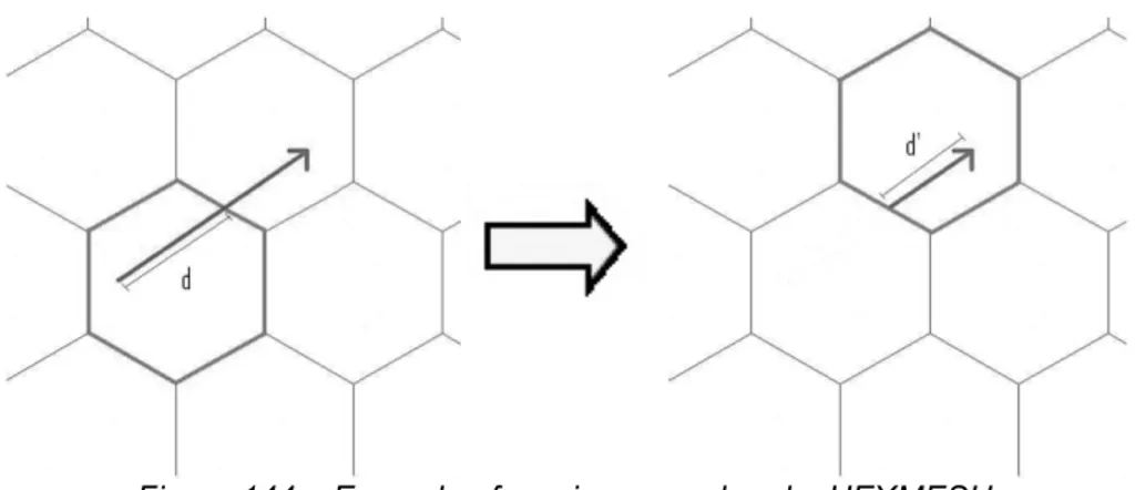
The basic functioning of the HEXMESH routine is analogous to the MCNP5 card FMESH mesh tally [17], i.e. a regular hexagonal prism lattice is superimposed on the MCNP5 ATUCHA-2 model and the contribution of each neutron track processed by MCNP5 is tallied in the crossed hexagonal prism. The hexagonal prism lattice was selected to match exactly the lattice used in NESTLE code nodalization. The HEXMESH routine calculates the flux φnode inside a node according to the formula used by MCNP5 to calculate the flux inside a cell [17],
where W is the total weight, V is node volume, wgtj is the weight of the single track and dj is the track length crossing the node, finally, summation is over all the track crossing the node.
Every neutron track simulated by MCNP5 is processed by the HEXMESH routine. The first step is to locate the track inside the hexagonal prism grid map, i.e. assign coordinates, then the track length crossing the mesh node is scored and the control is passed to the next node until the particle interaction (e.g. capture, fission, scattering) is extinguished. A 2D sketch of such procedure is shown in Figure 144.
Figure 144 – Example of scoring procedure by HEXMESH
An affine transformation algorithm calculates the hexagonal coordinates. It maps the original hexagonal map to a new coordinates system in which the assignment of hexagonal coordinates is easily calculated. Sketches of the affine transformations are reported in Figure 145 (different affine transformations are used for X and Y coordinate).
X coordinates Y coordinates
Figure 145 – Affine transformation method
The routine is fault tolerant about hexagonal location assignment because it checks if the track starting point is inside the selected hexagonal prism and if not (e.g. due to numerical round-off) a corrector subroutine moves the actual node to the correct location. The routine is programmed in C language and it is called
directly by the main MCNP5 FORTRAN90 routines using mixed C/FORTRAN language programming. A new card named ‘HTRAC’ was implemented to the MCNP5 command cards to enable the calling of the HEXMESH routine for each neutron track processed in the simulation.
B.1.3.
HEXMESH verification
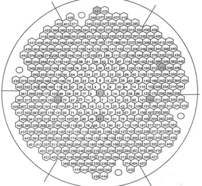
The verification test of the HEXMESH routine consisted of a comparison between the results calculated by HEXMESH routine and the standard output from MCNP5 flux tally F4. Six channels were tallied in several different core locations for a total of 60 node tallies (see Figure 146, the channel tallied are highlighted in dark grey).
Figure 146 – Selection of channel for HEXMESH verification
Several tests were done using different ATUCHA-2 models and a number of MCNP5 neutron histories. In most cases the results of MCNP5 F4 tally and HEXMESH routine match exactly to the 5-th significant digit confirming correct implementation of the HEXMESH routine. Occasional difference in the 5-th digit is due to numerical round-off error. The verification results are reported in Table 32.
Table 32 – HEXMESH verification results
Channel Case Lvl 1 Lvl 2 Lvl 3 Lvl 4 Lvl 5
HEXMESH 1.4049E-06 2.1431E-06 3.1880E-06 5.8362E-06 5.4481E-06 MCNP5 1.4050E-06 2.1431E-06 3.1880E-06 5.8362E-06 5.4481E-06 1
Diff [%] 0.000 0.000 0.000 0.000 0.000 HEXMESH 0.0000E+00 2.9542E-07 1.9546E-06 2.8463E-06 3.2809E-06
MCNP5 0.0000E+00 2.9542E-07 1.9546E-06 2.8463E-06 3.2809E-06 39
Diff [%] 0.000 0.000 0.000 0.000 0.000 HEXMESH 0.0000E+00 6.5574E-07 1.4088E-06 2.7493E-06 7.8754E-07
MCNP5 0.0000E+00 6.5574E-07 1.4088E-06 2.7493E-06 7.8754E-07 60
Diff [%] 0.000 0.000 0.000 0.000 0.000 HEXMESH 6.1669E-07 8.6043E-07 1.3497E-06 5.7311E-08 4.9653E-08
MCNP5 6.1669E-07 8.6043E-07 1.3497E-06 5.7311E-08 4.9653E-08 75
Diff [%] 0.000 0.000 0.000 0.000 0.000 HEXMESH 2.4749E-06 7.1765E-07 4.8761E-07 2.9502E-06 3.0853E-06
MCNP5 2.4749E-06 7.1765E-07 4.8761E-07 2.9502E-06 3.0853E-06 78
Diff [%] 0.000 0.000 0.000 0.000 0.000
Channel Case Lvl 6 Lvl 7 Lvl 8 Lvl 9 Lvl10
HEXMESH 4.1755E-06 6.1159E-06 9.0211E-06 5.8705E-06 3.4822E-06 MCNP5 4.1755E-06 6.1159E-06 9.0211E-06 5.8705E-06 3.4823E-06 1
Diff [%] 0.000 0.000 0.000 0.000 -0.003 HEXMESH 6.4675E-06 4.8495E-06 4.0327E-06 2.2923E-06 5.5517E-06
MCNP5 6.4675E-06 4.8495E-06 4.0327E-06 2.2923E-06 5.5518E-06 10
Diff [%] 0.000 0.000 0.000 0.000 -0.002 HEXMESH 4.1330E-07 3.3223E-07 6.0561E-07 4.0847E-07 0.0000E+00
MCNP5 4.1330E-07 3.3223E-07 6.0562E-07 4.0847E-07 0.0000E+00 39
Diff [%] 0.000 0.000 -0.002 0.000 0.000 HEXMESH 5.0903E-08 0.0000E+00 0.0000E+00 3.6251E-07 1.6925E-07
MCNP5 5.0903E-08 0.0000E+00 0.0000E+00 3.6251E-07 1.6925E-07 60
Diff [%] 0.000 0.000 0.000 0.000 0.000 HEXMESH 1.2883E-07 4.2284E-08 0.0000E+00 0.0000E+00 0.0000E+00
MCNP5 1.2883E-07 4.2284E-08 0.0000E+00 0.0000E+00 0.0000E+00 75
Diff [%] 0.000 0.000 0.000 0.000 0.000 HEXMESH 3.5597E-06 1.9662E-06 1.4192E-06 1.4427E-06 1.9973E-08
MCNP5 3.5597E-06 1.9662E-06 1.4192E-06 1.4427E-06 1.9973E-08 78
Diff [%] 0.000 0.000 0.000 0.000 0.000
B.1.4.
Convergence flux feature
The neutron flux convergence was checked using an additional feature of HEXMESH routine, i.e. the partial flux results from HEXMESH tally is printed-out each 150 active cycle for the diagnostic purposes.
B.2.
The tool for automating the NJOY processing
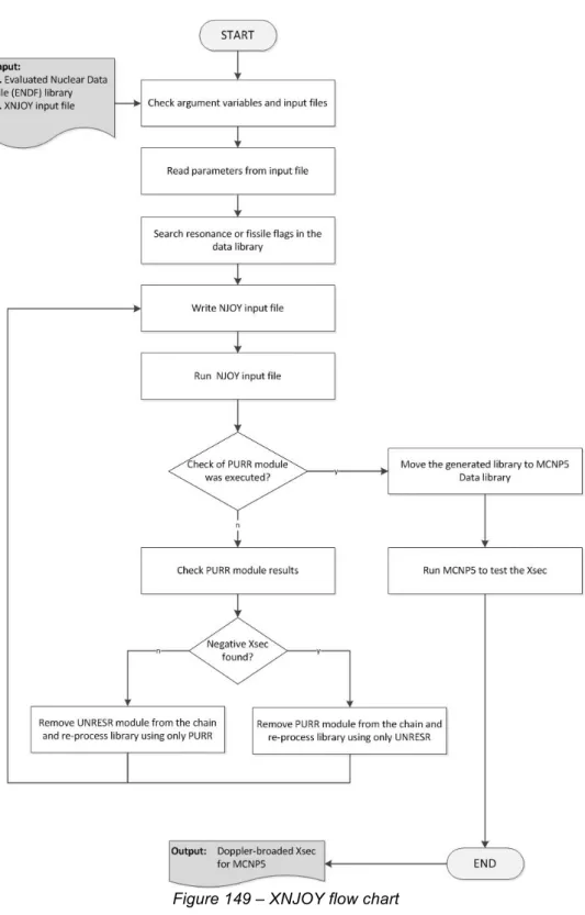
The computer program XNJOY was developed to manage all the process of Xsec generation using the NJOY code. The program automates the process of input deck creation, checks the processed nuclear library and executes MCNP as final check of the produced Xsec. This tool was necessary since multiple iterations of NJOY are required to set-up the Xsec library for simulation at BEQ with HFP core condition (more than 500 NJOY runs are required). Then, some modules do not execute consistency or error checks in the processed library. A case is the PURR module [18] that for a few isotopes could produce negative Xsec. The XNJOY program was written in C and PERL programming language.
Several routines are implemented to check the Xsec generated by the PURR module. The UNRESR module is used for diagnostic purpose. If the generated Xsec passes all the Xsec checks the UNRESR module is switched off and the
Xsec is generated again using only the PURR module. Otherwise the UNRESR module [18] is kept and the PURR module is excluded from the NJOY chain of modules. The following checks are implemented (see [18] for more detail about the following quantities):
• Xsec difference between PURR and UNRESR; • Calculated total Xsec to the total Xsec given by NJOY; • Bondarenko tables consistency;
• Probability table;
• Search for zero Xsec and calculate the cumulative probability; • Check for negative Xsec.
At the end of the processing a MCNP5 test case is run automatically to check if the Xsec was properly generated. All the data processing was tracked in the XNJOY output file, together with the results of checking routines. An output sample is reported to Figure 147 e Figure 148. A flow chart of the XNJOY program is reported in Figure 149.
Figure 147 – Comparison of UNRESR and PURR results
The generation of thermal library requires the use of the module LEAPR [18]. This module generates the thermal scattering data used by THERM module [18]. The thermal processing scheme is reported Figure 150.
Figure 150 – NJOY thermal Xsec processing
The standard MCNP5 data library includes thermal Xsec libraries to describe the thermal proprieties of most common moderators. However, few temperature are available. This level of detail was not enough for the application in this research. Hence, an interpolation process was implemented. Instead of interpolate the thermal Xsec, was chosen to interpolate the water spectral distributions used by the LEAPR code. This option was included in the XNJOY program.
B.3.
The tool for generating burnup dependent material
compositions
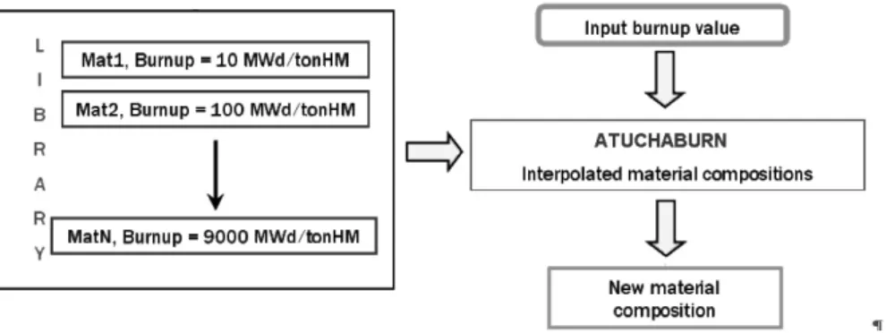
Implementation of BEQ core condition requires the implementation of the correspondent fuel burnup distribution inside the core. Such burnup data were provided by NA-SA [2]. The ATUCHABURN computer program was designed to calculate burnup dependent material compositions using a pre-calculated database of material compositions at several fixed burnup values. The program needs pre-calculated material compositions master library (MML). The MML was generated using the MONTEBURNS2.0 code [20]. A result of those calculations was a MML of material compositions for 56 burnup values ranging from 0 to 9000 MWd/tonHM (see APPENDIX E for more detail about the model and the procedure used). Each material composition contains 56 isotopes. The isotopes selected are the most relevant for ATUCHA-2 depletion calculation (see APPENDIX E).
A Lagrange polynomial interpolation scheme was implemented in the ATUCHABURN routine to calculate compositions at the desired burnup values from data contained in the MLL. The Lagrange polynomials satisfy the following condition:
Where, Li is the Lagrange polynomial of order i, (x0…xn) are the burnup values used MONTEBURNS2.0 simulations. The solution P(x) of the interpolation problem can be expressed directly in terms of the polynomials Li, leading to the Lagrange interpolation formula:
Where, fi is the calculated isotope composition at i burnup value (interpolation fixed point). The Lagrange’s formula is useful in this context since many interpolation problems are to be solved for the same support abscissa x but different sets of support ordinates fi. The ATUCHABURN routine working scheme is reported in the following figure:
Figure 151 – ATUCHABURN working scheme
ATUCHABURN was developed using the C computer programming language. Several families of interpolation fixed point can be selected when interpolation order is beyond linear interpolation (e.g. quadratic, cubic). For example, in case of quadratic interpolation, if i is the burnup nearest lower neighbor in the MML to the given input burnup value, hence 2 set of burnup value can be selected for interpolation:
• (i-1, i, i+1); • (i, i+1, i+2).
An example is reported in Figure 152 for quadratic interpolation case. A sensitivity analysis showed that the results are not dependent on this selection due to the smooth behavior of isotope mass trend versus burnup.
Figure 152 – Selection of range of MLL burnup value
The results calculated using linear, quadratic and cubic interpolation were compared. Comparison of criticality eigenvalue results showed a negligible difference (i.e. differences were inside the Monte Carlo statistical uncertainty). From the analysis of the masses of different material compositions, an anomalous trend was found for several isotopes using the cubic interpolation scheme. Such deviation was due to a numerical problem of oscillation at the edges of an interval that occurs when using polynomial interpolation with polynomials of high degree. Therefore, the cubic and higher order interpolation scheme were rejected. Finally, the linear and quadratic interpolations gave almost the same results. Thus, for sake of simplicity, linear interpolation was selected in this research.
B.4.
The tool for generating MCNP5 core input deck
The ATUCHACORE computer program, written in mixed computer language C/PERL, prepares the MCNP5 input deck in a fully automatic way using an input data provided by the user. Several parameters can be selected, the main feature are reported in the following list:
• Pre-defined core conditions (BEQ, BOL); • Different FA model can be loaded;
• 3 kinds of CR insertion can be used (ARO, ARI, critical CR configuration); • User defined number of axial layer;
• User defined number of composition for layer;
• User defined number of isotopes in the material composition; • User defined number of material composition;
• Optimization for representing the Boron cloud configuration.
The user has to provide an input text file plus several data files for material densities and material compositions (list of isotopes and weight fractions). A sample of the input deck with a description of the user-required parameters is reported in Figure 153.
Figure 153 – ATUCHACORE input deck
B.5.
The tool for generating minor fission product lumped
Xsec
Irradiation of nuclear fuel produces an accumulation of fission products (FP). The most relevant isotopes were directly considered in the simulations but the cumulative effect of the other FP could not be neglected. To take into account the effects of such FP, a procedure to lump these isotopes together in a pseudo fission product Xsec (p-Xsec) was developed, since MONTEBURNS2.0 does not have such capability. A special MCNP5 Xsec library including the contribution of all FP not directly took into account in the simulation was set up. The nuclear data are based on the ENDF/B-VII continuous energy library. The formula used to calculated an averaged cross section is the following,
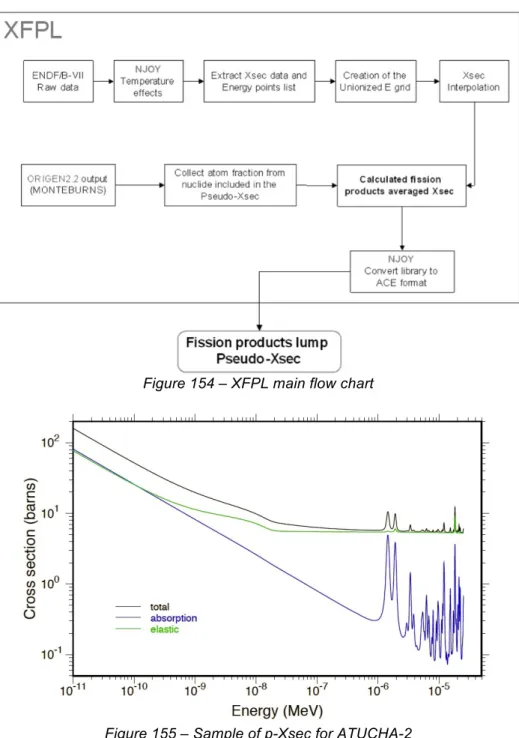
Where σPseudo is the p-Xsec of fission products, σi the nuclide Xsec and ni the isotope atom fraction, the processing is executed for continuous energies Xsec. The p-Xsec is calculated for each ENDF section file (MT) that contributes to total Xsec (MT = 1 in ENDF terminology [38]). This data is taken from ENDF/B-VII. The atom fractions are instead calculated from ORIGEN2.2 output collected by MONTEBURNS2.0. The computer routine XFPL, written in mixed programming language C/PERL, was developed to automate the process of creation and for checking the σPseudo. A flow chart describing the main steps of such procedure is reported in Figure 154. The NJOY99 code was used twice within such procedure,
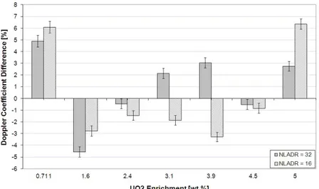
to consider temperature effects in the initial step and to convert the library to the ACE format in the last step. An example of p-Xsec correspondent to ATUCHA-2 average burnup is reported in Figure 155.
APPENDIX C.
CROSS SECTION VALIDATION
C.1.
NJOY parameter sensitivities
The NJOY input deck requires the user to set-up several parameters. A sensitivity analysis was set to investigate the effect of the main NJOY parameters used in this research. Description of the NJOY modules and parameters are reported in [18]. The sensitivity analysis was based on the “The Doppler-Defect Benchmark” [40], approved by the Joint Benchmark Committee of the Mathematics and Computations, Reactor Physics, and Radiation Protection and Shielding Divisions of the American Nuclear Society. The Doppler coefficient is very susceptible to Xsec variations, hence is an optimal benchmark to test the NJOY parameters.
C.1.1.
Overview of ‘The Doppler-Defect benchmark’
A set of computational benchmarks for the Doppler reactivity defect has been specified for fuel pin cells containing normal or enriched UO2 fuel, reactor-recycle mixed-oxide (MOx) fuel, or weapons-grade MOx fuel [40]. In this research only the normal or enriched UO2 fuel was considered. The benchmark specifications contain 2 pin cells for hot zero power (HZP) and hot full power (HFP) conditions, respectively. The pin cells are based on an “optimized” fuel assembly design that has been idealized in a number of ways to simplify the calculations. None of the idealizations have any significant impact on Doppler behavior. At HZP, the temperature for every material is a uniform 600 K. At HFP, the fuel temperature is raised to 900 K, keeping all the other material at 600 K. The Doppler-defect is calculated as the reactivity difference between HFP and HZP conditions. The Doppler coefficient (DC) is defined in the following formula:
where ΔTFuel is 300 K. The benchmark model and the correspondent MCNP5 model are reported in Figure 156. Geometry and material specification are reported in [40].
C.1.2.
Sensitivity on fractional reconstruction tolerance
The RECONR module reconstructs resonance cross sections using the resonance parameters and converts Xsec represented with non-linear interpolation schemes (such as lin-log, log-lin, log-log, etc.) to linear representation. The result is a point-wise ENDF file where all Xsec have been set on a unionized energy grid. All the Xsec are reconstructed to within a user specified accuracy. The level of accuracy can be set using the parameter ERR, defined as the fractional reconstruction tolerance. Such parameter is very important and it is used by other modules of NJOY, e.g. BROADR, THERMR, ACER, etc. It is recommended as good choice to use the same ERR value for all the modules. The reference ERR value was selected to be equal to 0.001. Sensitivity was done using the values of 0.1 and 0.0001. Appreciable difference was noticed in the data library memory storage. It was found a problem in the case of ERR = 0.0001 in both NJOY processing and MCNP5 simulations. It was found that too many energy points are generated using such small ERR value, hence, the results in this case were rejected. The effect of this parameter on Doppler coefficients is reported in Figure 157. It was found a relative difference from the reference case up to 6%.
Figure 157 – Sensitivity on ERR parameter
C.1.3.
Number of resonance ladders used in PURR module
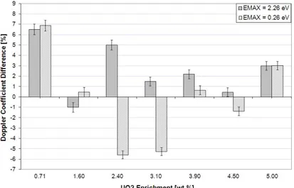
The PURR module is used to prepare the probability tables for the treatment of the unresolved resonance self-shielding in MCNP5. This module constructs a series of resonance ladders that obey the statistical distributions given in file 2 of the ENDF file [38]. Each of those ladders will be sampled randomly to produce contributions to a probability table. The probability tables depend on the number of resonance ladders. This number is selected changing the parameter NLADR. The reference NLADR value was selected to 64 resonance ladders. The effects on the Doppler coefficients is reported in Figure 158. A relative differences from reference case up to ~6% was found.
Figure 158 – Sensitivity on resonance ladder parameter
C.1.4.
Sensitivity on relevant THERM parameters
The LEAPR module of NJOY is used to prepare the scattering law S(α,β) and related quantities, which describe thermal neutron scattering from bound moderators, in the ENDF-6 format used by the THERMR module of NJOY. Relevant parameter were identified in the maximum energy for thermal treatment and the number of equal-probable bins
C.1.4.1 Sensitivity on EMAX parameter
The parameter EMAX defines the maximum energy to be used for the thermal scattering treatment. A value of 4.6 eV was selected as reference. Sensitivity was done decreasing such maximum energy by a step of 2 eV, i.e. 2.26 eV and 0.26 eV. The effects on the doppler coefficients is reported in Figure 159. Relative differences from reference case up to 7% were found. In the case of EMAX = 0.26 eV an appreciable effect on the calculated neutron flux was noticed, with a relative percentage difference of 3%.
Figure 159 – Sensitivity on maximum energy for thermal treatment
C.1.4.2 Sensitivity on NBIN parameter
The THERMR module calculates the angular dependence of scattering cosine by subdividing the cosine range until the actual angular function is represented by linear interpolation to within a specified tolerance. The integral under this curve is used in calculating the secondary-energy dependence [18]. Rather than providing the traditional Legendre coefficients, THERMR divides the angular range into equally probable cosine bins and then selects the single cosine in each bin that preserves the average cosine in the bin. These equally probable cosines can be converted to Legendre coefficients easily when producing group constants. The number of bins to use for the equally probable bins for the outgoing neutron spectra is defined by NBIN. The reference value was set NBIN = 16. Sensitivity was done reducing the NBIN parameter dividing a factor 2, i.e. NBIN = 8 and NBIN = 4. The effect on Doppler coefficient is reported in Figure 160. In both case the relative difference thermal neutron flux was quantify to a 5%.
Figure 160 – Sensitivity on equally probable angular bin
C.1.5.
Benchmark results
The final Xsec were used to calculate the Doppler coefficient. Then, the results were compared to other participants to the benchmark from international institute [47]. Results of comparison are reported in Figure 161, in which the “GNRSPG-ENDF/B-VIv8” identifies the results using the procedure developed in this research. The calculated Doppler coefficients are in good agreement to the other participants.
C.2.
Cross section validation
Benchmarking the new libraries is an important step in the development of a validated application library. In April 1999 Los Alamos National Laboratory released a suite of 86 criticality benchmarks [41] (along with the corresponding MCNP input files) for the specific purpose of validating nuclear data libraries for MCNP. This suite of criticality benchmark was used to validate the Xsec generation methodology.
C.2.1.
Description of the criticality benchmark validation suite
The benchmarks in the suite were specifically chosen to obtain a set of problems that would test different energy regions, such as the high-energy region of fast critical assemblies and the thermal region of the solution experiments, to test various reflector materials while maintaining an acceptable amount of benchmark problems.
This suite has been compiled using the International Criticality Safety Benchmark Evaluation Project (ICSBEP). This suite is a compendium of criticality experimental information. The geometry and material specifications for the 86 benchmarks were taken from the ICSBEP compendium. The criticality models are collected in 5 different categories:
• Critical assemblies with 233U; • Intermediate enriched 235U (IEU); • Highly enriched 235U (HEU);
• 239Pu and mixed metal assemblies (MM). The list of criticality benchmarks is reported in Table 33.
Table 33 – Criticality benchmark descriptions
Name Type Description ICSBEP
Identification label
23umt1 U233 Jezebel-23, Bare Sphere of U233 233U-MET-FAST-001 23umt2a U233 0.481" HEU-Reflected Sphere of
U233; Planet Assembly
233U-MET-FAST-002 Case 1 23umt2b U233 0.783" HEU-Reflected Sphere of
U233, Planet Assembly
233U-MET-FAST-002 Case 2 23umt3a U233
0.906" Normal Uranium-Reflected Sphere of U233, Planet Assembly
233U-MET-FAST-003 Case 1 23umt3b U233
2.09" Normal Uranium-Reflected Sphere of U233, Planet
Assembly
233U-MET-FAST-003 Case 2 23umt4a U233
0.96" Tungsten-Reflected Sphere of U233, Planet Assembly
233U-MET-FAST-004 Case 1 23umt4b U233
2.28" Tungsten-Reflected Sphere of U233, Planet Assembly
233U-MET-FAST-004 Case 2 23umt5a U233 0.805" Be-Reflected Sphere of
U233, Planet Assembly
233U-MET-FAST-005 Case 1 23umt5b U233 1.652" Be-Reflected Sphere of U233, Planet Assembly 233U-MET-FAST-005 Case 2
23umt6 U233
Flattop-23, 7.84" Normal-Uranium Reflected Sphere of U233
233U-MET-FAST-006 flat23 U233 Flattop-23, CSEWG,
U(N)-reflected U233 sphere + gap F-24 (CSEWG) 23usl1a U233
ORNL-5, 1.0226 g/l Unreflected 27.24" Sphere of U233 nitrate solution
233U-SOL-THERM-001 Case 1 23usl1b U233
ORNL-6, 1.0253 g/l Unreflected 27.24" Sphere of U233 nitrate solution withBoron
233U-SOL-THERM-001 Case 2 23usl1c U233
ORNL-7, 1.0274 g/l Unreflected 27.24" Sphere of U233 nitrate solution withBoron
233U-SOL-THERM-001 Case 3 23usl1d U233
ORNL-8, 1.0275 g/l Unreflected 27.24" Sphere of U233 nitrate solution withBoron
233U-SOL-THERM-001 Case 4 23usl1e U233
ORNL-9, 1.0286 g/l Unreflected 27.24" Sphere of U233 nitrate solution withBoron
233U-SOL-THERM-001 Case 5
23usl8 U233
ORNL-11, 1.0153 g/l
Unreflected 48.04" Sphere of U233 nitrate solution withBoron
233U-SOL-THERM-008 ieumt1a IEU Jemima 1, Cylindrical Disks of
HEU and Natural Uranium
IEU-MET-FAST-001 Case 1 ieumt1b IEU Jemima 2, Cylindrical Disks of
HEU and Natural Uranium
IEU-MET-FAST-001 Case 2 ieumt1c IEU Jemima 3, Cylindrical Disks of
HEU and Natural Uranium
IEU-MET-FAST-001 Case 3 ieumt1d IEU Jemima 4, Cylindrical Disks of HEU and Natural Uranium IEU-MET-FAST-001 Case 4
ieumt2 IEU
Reflected Jemima, U(N)-Reflected Cylindrical Disks of HEU and Natural Uranium
IEU-MET-FAST-002 ieumt3 IEU Bare IEU Sphere (36 wt.%), VNIIEF IEU-MET-FAST-003 ieumt4 IEU Graphite-Reflected IEU Sphere (36 wt.%), VNIIEF IEU-MET-FAST-004 ieumt5 IEU Steel-Reflected IEU Sphere (36 wt.%), VNIIEF IEU-MET-FAST-005 ieumt6 IEU Duralumin-Reflected IEU
Sphere (36 wt.%), VNIIEF IEU-MET-FAST-006 umet1ss HEU
Godiva, Unreflected sphere of HEU, Simple Sphere
representation
HEU-MET-FAST-001 Case a umet1ns HEU
Godiva, Unreflected sphere of HEU, Nested Spherical shell representation
HEU-MET-FAST-001 Case b bigten1 HEU BIGTEN, 1d model: U(N)
reflected uranium sphere F-10 (CSEWG) bigten2 HEU BIGTEN, 2d model: U(N) reflected uranium cylinder F-10 (CSEWG)
umet3a HEU
2" Tuballoy-Reflected HEU(93.5) Sphere, Topsy Assembly
HEU-MET-FAST-003 Case 1
umet3b HEU
3" Tuballoy-Reflected HEU(93.5) Sphere, Topsy Assembly
HEU-MET-FAST-003 Case 2
umet3c HEU
4" Tuballoy-Reflected HEU(93.5) Sphere, Topsy Assembly
HEU-MET-FAST-003 Case 3
umet3d HEU
5" Tuballoy-Reflected HEU(93.5) Sphere, Topsy Assembly
HEU-MET-FAST-003 Case 4 7" Tuballoy-Reflected
umet3f HEU
8" Tuballoy-Reflected HEU(93.5) Sphere, Topsy Assembly
HEU-MET-FAST-003 Case 6
umet3g HEU
11" Tuballoy-Reflected HEU(93.5) Sphere, Topsy Assembly
HEU-MET-FAST-003 Case 7
umet3h HEU
1.9" Tungsten Carbide-Reflected HEU(93.5) Sphere, Topsy Assembly
HEU-MET-FAST-003 Case 8 umet3i HEU
2.9" Tungsten Carbide-Reflected HEU(93.5) Sphere, Topsy Assembly
HEU-MET-FAST-003 Case 9 umet3j HEU
4.5" Tungsten Carbide-Reflected HEU(93.5) Sphere, Topsy Assembly
HEU-MET-FAST-003 Case 10
umet3k HEU
6.5" Tungsten Carbide-Reflected HEU(93.5) Sphere, Topsy Assembly
HEU-MET-FAST-003 Case 11 umet3l HEU 8.0" Nickel-Reflected HEU(93.5)
Sphere, Topsy Assembly
HEU-MET-FAST-003 Case 12 umet4a HEU Water-Reflected HEU(97.675) Sphere, with plexiglass ring HEU-MET-FAST-004 Case 2
umet4b HEU
Water-Reflected HEU(97.675) Sphere, Trans. Am. Nuc. Soc. 27, pg. 412 (1977)
HEU-MET-FAST-004 (Case 1) umet8 HEU Bare HEU Sphere, VNIITF, 3D
model HEU-MET-FAST-008
umet9a HEU Be-Reflected HEU(~89.6) Sphere, VNIITF HEU-MET-FAST-009 Case 1 umet9b HEU BeO-Reflected HEU(~89.6)
Sphere, VNIITF
HEU-MET-FAST-009 Case 2 umet11 HEU Polyethylene (CH2)-Reflected
HEU(~89.6) Sphere, VNIITF HEU-MET-FAST-011 umet12 HEU Aluminium-Reflected HEU(~89.6) Sphere, VNIITF HEU-MET-FAST-012 umet13 HEU St.20 Steel-Reflected
HEU(~89.6) Sphere, VNIITF HEU-MET-FAST-013 umet14 HEU Depleted Uranium-Reflected HEU(~89.6) Sphere, VNIITF HEU-MET-FAST-014 umet15 HEU Bare HEU Cylinder, VNIITF HEU-MET-FAST-015 umet18 HEU Simplified Bare HEU Sphere, VNIIEF HEU-MET-FAST-018 umet19 HEU Graphite-Reflected HEU
Sphere, VNIIEF HEU-MET-FAST-019
umet20 HEU Polyethylene-Reflected HEU
umet21 HEU Steel-Reflected HEU Sphere,
VNIIEF HEU-MET-FAST-021
umet22 HEU Duralumin-Reflected HEU Sphere, VNIIEF HEU-MET-FAST-022 umet28 HEU Flattop-25, U(nat)-Reflected
HEU SPHERE HEU-MET-FAST-028
usol13a HEU ORNL-1, Unreflected Sphere of Uranyl(20.12 g/l) Nitrate
HEU-SOL-THERM-003 Case 1 usol13b HEU
ORNL-2, Unreflected Sphere of Uranyl(23.53 g/l) Nitrate with Boron
HEU-SOL-THERM-003 Case 2 usol13c HEU
ORNL-3, Unreflected Sphere of Uranyl(26.77 g/l) Nitrate with Boron
HEU-SOL-THERM-003 Case 3 usol13d HEU
ORNL-4, Unreflected Sphere of Uranyl(28.45 g/l) Nitrate with Boron
HEU-SOL-THERM-003 Case 4 usol32 HEU
ORNL-10, Unreflected Sphere of Uranyl(28.45 g/l) Nitrate with Boron
HEU-SOL-THERM-032 pumet1 239Pu Jezebel-Pu (4.5%), Bare sphere
of Pu-239 with 4.5% Pu-240 PU-MET-FAST-001 pumet2 239Pu Jezebel-Pu (20%), Bare sphere of Pu-239 with 20% Pu-240 PU-MET-FAST-002 pumet5 239Pu Tungsten-Reflected Pu(94.79)
Sphere, Planet assembly PU-MET-FAST-005 pumet6 239Pu
Normal Uranium-Reflected Pu(93.80) Sphere, Flattop assembly
PU-MET-FAST-006 pumet8a 239Pu
Thorium-Reflected Pu(93.59) Sphere, Thor Assembly, 1D Model
PU-MET-FAST-008 Case 1 pumet8b 239Pu
Thorium-Reflected Pu(93.59) Sphere, Thor Assembly, 2D Model
PU-MET-FAST-008 Case 2 pumet9 239Pu Aluminum-Reflected Pu(94.8)
Sphere, Comet Assembly PU-MET-FAST-009
C.2.2.
Validation of generated Xsec
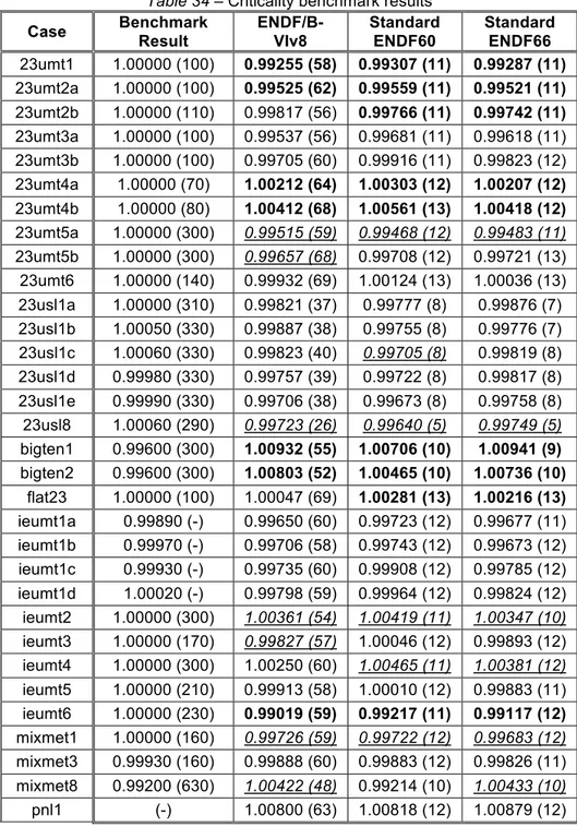
The ENDF/B-VIv8 data were processed by the XNJOY program and MCNP5 calculation were executed. The results are reported in Table 34, together with the benchmark results and the reference results from the standard ENDF60 and ENDF66 libraries contained in the MCNP5 standard Xsec library [17]. Two results were rejected since errors were found in the MCNP5 input deck. Those cases are
higher than 1σ is reported in Table 35. The results showed that the Xsec processed have an acceptable level of validation for the purpose of this research.
Table 34 – Criticality benchmark results
Case Benchmark Result ENDF/B-VIv8 Standard ENDF60 Standard ENDF66 23umt1 1.00000 (100) 0.99255 (58) 0.99307 (11) 0.99287 (11) 23umt2a 1.00000 (100) 0.99525 (62) 0.99559 (11) 0.99521 (11) 23umt2b 1.00000 (110) 0.99817 (56) 0.99766 (11) 0.99742 (11) 23umt3a 1.00000 (100) 0.99537 (56) 0.99681 (11) 0.99618 (11) 23umt3b 1.00000 (100) 0.99705 (60) 0.99916 (11) 0.99823 (12) 23umt4a 1.00000 (70) 1.00212 (64) 1.00303 (12) 1.00207 (12) 23umt4b 1.00000 (80) 1.00412 (68) 1.00561 (13) 1.00418 (12) 23umt5a 1.00000 (300) 0.99515 (59) 0.99468 (12) 0.99483 (11) 23umt5b 1.00000 (300) 0.99657 (68) 0.99708 (12) 0.99721 (13) 23umt6 1.00000 (140) 0.99932 (69) 1.00124 (13) 1.00036 (13) 23usl1a 1.00000 (310) 0.99821 (37) 0.99777 (8) 0.99876 (7) 23usl1b 1.00050 (330) 0.99887 (38) 0.99755 (8) 0.99776 (7) 23usl1c 1.00060 (330) 0.99823 (40) 0.99705 (8) 0.99819 (8) 23usl1d 0.99980 (330) 0.99757 (39) 0.99722 (8) 0.99817 (8) 23usl1e 0.99990 (330) 0.99706 (38) 0.99673 (8) 0.99758 (8) 23usl8 1.00060 (290) 0.99723 (26) 0.99640 (5) 0.99749 (5) bigten1 0.99600 (300) 1.00932 (55) 1.00706 (10) 1.00941 (9) bigten2 0.99600 (300) 1.00803 (52) 1.00465 (10) 1.00736 (10) flat23 1.00000 (100) 1.00047 (69) 1.00281 (13) 1.00216 (13) ieumt1a 0.99890 (-) 0.99650 (60) 0.99723 (12) 0.99677 (11) ieumt1b 0.99970 (-) 0.99706 (58) 0.99743 (12) 0.99673 (12) ieumt1c 0.99930 (-) 0.99735 (60) 0.99908 (12) 0.99785 (12) ieumt1d 1.00020 (-) 0.99798 (59) 0.99964 (12) 0.99824 (12) ieumt2 1.00000 (300) 1.00361 (54) 1.00419 (11) 1.00347 (10) ieumt3 1.00000 (170) 0.99827 (57) 1.00046 (12) 0.99893 (12) ieumt4 1.00000 (300) 1.00250 (60) 1.00465 (11) 1.00381 (12) ieumt5 1.00000 (210) 0.99913 (58) 1.00010 (12) 0.99883 (11) ieumt6 1.00000 (230) 0.99019 (59) 0.99217 (11) 0.99117 (12) mixmet1 1.00000 (160) 0.99726 (59) 0.99722 (12) 0.99683 (12) mixmet3 0.99930 (160) 0.99888 (60) 0.99883 (12) 0.99826 (11) mixmet8 0.99200 (630) 1.00422 (48) 0.99214 (10) 1.00433 (10) pnl1 (-) 1.00800 (63) 1.00818 (12) 1.00879 (12)
pnl6 (-) 1.00308 (68) 1.00327 (13) 1.00354 (14) pumet1 1.00000 (200) 0.99799 (53) 0.99781 (11) 0.99750 (11) pumet10 1.00000 (180) 0.99869 (67) 1.00014 (12) 0.99866 (12) pumet11 1.00000 (100) 0.99581 (73) 0.99753 (14) 0.99695 (14) pumet18 1.00000 (300) 0.99940 (65) 0.99968 (12) 0.99917 (12) pumet19 0.99920 (150) (-) 1.00208 (12) 1.00126 (13) pumet2 1.00000 (200) 0.99808 (56) 0.99853 (11) 0.99805 (11) pumet20 0.99930 (170) 0.99888 (68) 1.00002 (12) 0.99848 (13) pumet21a 1.00000 (260) 0.99689 (62) 1.00452 (13) 1.00407 (12) pumet21b 1.00000 (260) 0.99772 (64) 0.99324 (12) 0.99252 (13) pumet22 1.00000 (210) 0.99944 (63) 0.99658 (11) 0.99614 (12) pumet23 1.00000 (200) 0.99709 (56) 0.99829 (11) 0.99786 (12) pumet24 1.00000 (200) 0.99642 (60) 1.00002 (12) 0.99986 (13) pumet25 1.00000 (200) 1.00793 (65) 0.99709 (11) 0.99659 (12) pumet26 1.00000 (240) 1.00273 (70) 0.99742 (12) 0.99663 (12) pumet5 1.00000 (130) 1.00613 (67) 1.00964 (12) 1.00770 (12) pumet6 1.00000 (300) 1.00492 (62) 1.00396 (14) 1.00253 (14) pumet8a 1.00000 (300) 1.00221 (58) 1.00658 (13) 1.00666 (12) pumet8b 1.00000 (60) 1.00480 (65) 1.00603 (12) 1.00574 (12) pumet9 1.00000 (270) 0.99168 (63) 1.00111 (12) 1.00114 (12) pusl11a 1.00000 (520) 0.99463 (54) 0.99543 (10) 0.99617 (10) pusl11b 1.00000 (520) 1.00011 (59) 1.00080 (11) 1.00132 (11) pusl11c 1.00000 (520) 1.00633 (62) 1.00612 (12) 1.00648 (12) pusl11d 1.00000 (520) (-) 1.01031 (12) 1.01107 (12) umet11 0.99890 (150) 0.99510 (78) 0.99645 (15) 0.99513 (14) umet12 0.99920 (180) 0.99465 (58) 0.99391 (12) 0.99380 (12) umet13 0.99900 (150) 0.99336 (59) 0.99418 (11) 0.99405 (12) umet14 0.99890 (170) 0.99400 (56) 0.99553 (12) 0.99433 (12) umet15 0.99960 (170) 0.99224 (59) 0.99150 (12) 0.99109 (11) umet18 1.00000 (160) 0.99667 (60) 0.99616 (11) 0.99605 (12) umet19 1.00000 (300) 1.00354 (60) 1.00364 (12) 1.00344 (12) umet1ns 1.00000 (100) 0.99646 (57) 0.99656 (12) 0.99645 (11) umet1ss 1.00000 (100) 0.99671 (55) 0.99655 (11) 0.99647 (11) umet20 1.00000 (300) 0.99713 (67) 0.99741 (13) 0.99658 (13) umet21 1.00000 (260) 0.99406 (57) 0.99488 (12) 0.99401 (12) umet22 1.00000 (210) 0.99199 (61) 0.99230 (12) 0.99238 (11)
umet3a 1.00000 (500) 0.99051 (59) 0.99308 (12) 0.99170 (11) umet3b 1.00000 (500) 0.99148 (60) 0.99276 (11) 0.99180 (12) umet3c 1.00000 (500) 0.99713 (63) 0.99792 (12) 0.99686 (12) umet3d 1.00000 (300) 0.99402 (60) 0.99664 (12) 0.99523 (12) umet3e 1.00000 (300) 1.00073 (66) 1.00106 (13) 1.00028 (12) umet3f 1.00000 (300) 1.00078 (66) 1.00156 (12) 1.00066 (13) umet3g 1.00000 (300) 1.00172 (62) 1.00183 (13) 1.00142 (13) umet3h 1.00000 (500) 1.00353 (63) 1.00635 (12) 1.00464 (12) umet3i 1.00000 (500) 1.00616 (60) 1.00656 (13) 1.00582 (12) umet3j 1.00000 (500) 1.00943 (60) 1.00768 (12) 1.00917 (12) umet3k 1.00000 (500) 1.01270 (64) 1.00985 (12) 1.01351 (12) umet3l 1.00000 (300) 1.00469 (60) 1.00468 (12) 1.00433 (12) umet4a 1.00200 (-) 0.99925 (77) 1.00082 (14) 0.99961 (15) umet4b 1.00030 (50) 0.99390 (77) 0.99634 (15) 0.99578 (15) umet8 0.99890 (160) 0.99268 (54) 0.99243 (11) 0.99221 (12) umet9a 0.99920 (150) 0.99404 (61) 0.99482 (13) 0.99505 (13) umet9b 0.99920 (150) 0.99323 (64) 0.99381 (12) 0.99363 (12) usol13a 1.00120 (260) 0.99919 (38) 0.99789 (8) 0.99953 (7) usol13b 1.00070 (360) 0.99741 (40) 0.99700 (8) 0.99850 (8) usol13c 1.00090 (360) 0.99466 (42) 0.99357 (8) 0.99487 (9) usol13d 1.00030 (360) 0.99616 (44) 0.99506 (9) 0.99648 (8) usol32 1.00150 (260) 0.99880 (25) 0.99749 (6) 0.99915 (6) σ< |Δk| ≤2σ |Δk| > 2σ
Table 35 – Summary of cases with deviation higher than 1σ
Num #cases 1σ<|Δk|≤ 2σ #cases |Δk|>2σ ENDF/B-VIv8 25 22 ENDF60 31 21 ENDF66 24 24
APPENDIX D.
SENSITIVITIES ON MCNP5 PARAMETERS
In this Appendix are reported the following sensitivities concerning the MCNP criticality parameters:
• FC geometrical modeling;
• Initialization of neutron source energy distribution; • Selection of nominal source histories per cycle; • Selection boundary conditions for cell simulation; • Material FC representation for BEQ core simulation; • Use of a parallel environment.
D.1.
FC geometrical modeling
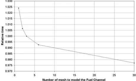
The optimal MCNP5 geometrical mesh for the FC structure was investigated. The results of a Monte Carlo calculation should not be affected by the kind of geometrical representation used, however, it is possible to save computer time using an appropriate geometrical mesh (here the term ‘mesh’ has to be intended as geometrical representation). The computer time trend against MCNP5 mesh number used to model a FA model is reported in Figure 162. From these sensitivities two different mesh grouping of fuel pins were used in the simulations. The FA model was represented using 6 MCNP5 mesh zone, then, one MCNP5 mesh zone for the representation of FA in the core simulation. Those FA models are reported in Par. 5.5.1.1.
Figure 162 – Computer time trend against MCNP5 mesh number
D.2.
Initialization of neutron source energy distribution
the default option used to initialize neutron energy [17]. Another method is to run a preliminary calculation with less neutron histories number in order to get a spatial converged neutron energy distribution representative of the system to be simulate. The latter method assures a better guess initial distribution for the simulation, hence, better accuracy and a quicker convergence. Sensitivity was done to compare the 2 methods. The criticality eigenvalue convergence and Shannon entropy behaviors are reported in Figure 163 and Figure 164, respectively. As expected the convergence is quicker using an educated initial guess neutron distribution. This can be seen analyzing the relative entropy of source. This difference is magnified in core simulations; in particular, a combination of educated guess distribution using an initial KSRC distribution in the preliminary calculation can further improve the convergence speed.
Figure 163 – Comparison of kinf trend
D.3.
Selection of nominal source histories per cycle
In MCNP5 criticality calculation are initialized using the KCODE criticality source card. A fundamental parameter is the nominal source histories per cycle (NSRCK parameter [17]). The effect of such parameter was investigated using several values for the NSRCK parameter. In each case the total number of histories was preserved. Results showed that for ATUCHA-2 system a high number of starting source histories for cycle has to be selected for the convergence of the entropy of source and criticality eigenvalue (see Figure 165 and Figure 166). It was noticed that for the system under investigation a number of histories per cycle below 10000 does not assure the same level of convergence at fixed total number of histories and computer resources.
D.4.
Selection boundary conditions for cell simulation
The FA model allows the investigation of several nuclear proprieties of the system neglecting the leakage (infinitive system). In this case a boundary condition has to be selected to manage the neutron reaching the model boundary. The MCNP5 code allows 3 options reported in Table 36, then, a representation of such boundary reflection scheme sketch of those configurations is reported in Figure 167:
Table 36 – FA boundary condition options
Boundary case Method of reflection for incoming neutron to the model boundary
Mirror Mirror reflection
White The angle of reflection is randomly chosen Periodic Same angle but the neutron starts in the opposing surface symmetrically
Mirror White Periodic
Figure 167 – Example of reflective boundary conditions
The effect of such boundary condition to criticality eigenvalue and neutron flux was investigated. Results are reported in Table 37. The periodic case was taken as reference since it is physically the most correct. The white and periodic cases are equivalent at this level of accuracy since the differences lay within the statistical uncertainty. The reflective case showed a difference beyond the statistical uncertainty, however such difference was small. The periodic boundary parameter was selected for FA simulation.
Table 37 – Initial conditions for the reference cases
Boundary case Kinf [pcm] Thermal flux Diff [%] Fast flux Diff [%]
Reflective +20 2.5E-02 1.5E-02
D.5.
FC representation for BEQ core simulation
Two FC model were tested to represent the fuel characteristic at BEQ core condition. The first model is the same used for the MONTEBURNS2.0 burnup calculation (see APPENDIX E), in which the fuel pin materials of a FC are represented using 4 different materials (i.e. each fuel pin material of a fuel ring is described by the same material). This model will be referred as A1. The second model represents the fuel with only one fuel material composition that is the homogenization from the material used for A1 model. The latter model will be referred as A2 model. These models are reported in Figure 168.
A1 FC model A2 FC model
Figure 168 – MCNP5 FA models used to model BEQ condition
A complete characterization of ATUCHA-2 nuclear fuel materials at BEQ using the detailed model A1 requires 18040 material compositions (4510 burnup values x 4 annular rings). MCNP5 simulations using an high number of material compositions requires huge amount of computer time and an higher number of histories to get acceptable statistical convergence. Thus, sensitivity was done to investigate if the A2 model could represent the characteristics of BEQ condition.
The neutron flux and the criticality eigenvalue results from FC A1 and A2 models were compared. The materials compositions corresponding to ATUCHA-2 average burnup value of ~4100 MWd/tonHM were selected. The difference in criticality eigenvalue was of 58 ± 13 pcm. Then, the relative and absolute flux differences are reported in Figure 169 and Figure 170, respectively. In the latter case the MCNP5 fluxes were normalized with the average ATUCHA-2 values of ~1014 n/(cm2s1). Results showed that the differences between the 2 models are low. From those results, the A2 model was selected. This model is good compromise between representation detail and use of computer resources and it allows a huge simplification of the ATUCHA-2 core model.
Figure 169 – Relative flux difference between A1 and A2 models
Figure 170 – Absolute flux difference between A1 and A2 models
D.6.
Use of a parallel environment
ATUCHA-2 core calculation at BEQ with HFP core conditions requires huge computer resources. To speed up the results MCNP5 was installed in a computer cluster machine. In a parallel environment the neutron number of histories are divided to each processor since each neutron history is run independently. A computer cluster consisting of 8 processor of current generation computer [36] was used in this research. A feature of MCNP5 code is the capability to use the full resources of parallel environment using the Message Passing Interface (MPI)
paradigm. Several compiling option parameters were tested to find the optimal performance for the cluster machine used in this research. The MCNP5 performance in a parallel environment was investigated using the ‘Speed up’ and ‘Efficiency’ functions. Those function are defined by the following formulas:
Where n is the number of processor used in the simulation. The results are reported in Table 38.
Table 38 – Speed test for parallel environment
Number of processors Time [s] Speed up Efficiency [%] 1 639 1.00 100.0 2 324 1.97 98.6 3 218 2.93 97.7 4 169 3.78 94.5 5 137 4.66 93.3 6 116 5.51 91.8 7 102 6.26 89.5
The performance of the cluster machine drastically decreases when the MCNP5 model exceeds a threshold number of cell region (around 50000). The system memory usage was checked and no anomalies were found. In those cases the MPI resource was not used. A final concern is that the reason of such problem should be investigated in detail since the use of parallel environment to investigate very complex systems is a key feature of Monte Carlo based neutron transport codes.
APPENDIX E.
BURNUP PROCEDURES
In this APPENDIX is reported the MONTEBURNS2.0 methodology, the code improvements and the qualification activity for calculation of burnup dependent material compositions.
E.1.
MCNP5 FA model for burnup simulation
The MCNP5 model used for burnup calculation represents the fuel pin compositions with 4 different materials. The criterion of grouping is the belonging of a fuel pin to one of the different 4 annular rings. Such modeling allows tracking the differences in fuel materials due to heterogeneous flux distribution over the FA during MONTEBURNS2.0 iterative process, hence, giving more accurate results. The MCNP5 model corresponds to the A1 model reported in APPENDIX D (section D.5.).
E.2.
MONTEBURN2.0 simulation parameters
The MONTEBURNS2.0 code requires the setting up of several burnup parameters [20]. The most relevant are summarized in Table 39. Other parameters concerned the MCNP5 calculation. The KCODE option was used, setting 50000 particles per cycle for 560 cycles, thus resulting in a total of 2.5 x 10⁷ histories simulated. The first 60 cycles were discarded for improving the final result statistics. The initial neutron source distribution was set using the KSRC card (MONTEBURNS2.0 does not allow the use of an educated initial guess of source neutron distribution). Sensitivity about the number of neutron history was done to check the accuracy of the calculated fluxes and 1-group Xsec. A higher number of histories modified the results of a factor 0.03%±0.01%. Periodic boundary conditions were selected (see APPENDIX D (section D.4.). The nuclear data library used is the continuous energy ENDF/B-VI release 8, processed by the NJOY99 code at HFP BIC.
Table 39 – MONTEBURNS2.0 main parameter description
Parameter Description
Total power of the system Power generated by the entire system represented in the MCNP5 model Total number of days burned Number represents the irradiation length of time in ORIGEN2.2
Number of outer burn steps Number indicates haw many iterative steps are desired
Identifier for ORIGEN2.2 library Identifies the initial ORIGEN2.2 Xsec data library
Recoverable energy per fission Recoverable energy for
235U for the system simulated
Number and list of automatic tally isotopes for each material
Libraries are updated only for isotopes in the list
E.3.
Selection of the MONTEBURNS relevant isotopes for
ATUCHA-2
MONTEBURNS2.0 simulations are very time consuming due to iterative process involving MCNP5 neutron transport calculations. The speed of each MCNP5 simulation is strongly affected by the number of isotope used by MONTEBURNS2.0 to update the ORIGEN2.2 library, hence, the selection of which material has to be considered as a relevant issue. Sensitivities analyses about the number of relevant isotopes to be included were performed. In this way, an optimal ratio between accuracy of the simulation and computational time was achieved. The following formula was used to select the ‘importance’ of a single nuclide:
where Nisotope is the atom density of a nuclide, σ the absorption and fission Xsec and threshold a value ranging from a minimum value of 10-10. The threshold value was increased up to the value of 10-4. In each case the correspondent number of relevant isotopes decreased. Then, the relative difference in criticality eigenvalue and isotopes mass production was compared to the most accurate case (99 isotopes). Sensitivity results are reported in Table 40.
Table 40 – Effects of relevant isotopes selection to kinf and mass production
Threshold Value Number of relevant isotopes MAX kinf diff. [%] MAX isotope gram diff. [%] 1.0e-10 99 - - 1.0e-9 75 3*10-4 ~10-3 1.0e-6 56 3*10-4 ~10-3 1.0e-5 30 6*10-4 ~10-2 1.0e-4 20 ~10-2 ~10-1
The case with 56 isotopes was selected and the corresponding list of isotopes is reported in Table 41, where Z is the atomic number and A the mass number.
Table 41 – Selected nuclides for the ATUCHA-2 burnup simulations
Element Z A Element Z A Element Z A
B 5 10 Pr 59 141 U 92 236 B 5 11 Pr 59 143 U 92 237 O 8 16 Nd 60 143 U 92 238 Kr 36 83 Nd 60 145 Np 93 237 Zr 40 93 Nd 60 147 Np 93 239 Tc 43 99 Pm 61 147 Pu 94 238 Ru 44 101 Pm 61 148 Pu 94 239