Mobile robots:localization and mapping alogorithms

(1)

(2)

(3)

A Maria Emilia, Pap`

a, Mamma e Dik,

voi tutti neanche immaginate quanto siate importanti per me.

(4)

(5)

Abstract

In recent years, mobile robots start to be very often used in various applica-tions involving home automation, planetary exploration, regions surveillance, rescue missions, ruins exploration. In all these fields, to accomplish its tasks, a mobile robot needs to navigate into an environment facing the localization, mapping and path planning problems. In this thesis a set of new algorithms to solve the mobile robots localization and mapping problems are proposed.

The aim is to provide an accurate mobile robot estimated pose and to build a reliable map for the environment where the robot moves, ensuring algorithms computational costs low enough so that the algorithms can be used in real time, while the robot is moving. The localization problem is faced in static and dynamic contexts, assuming the environment surround-ing the robot completely known, partially known or totally unknown. In the static context, localization algorithms based on the use of cameras and in-ertial measurement units are proposed. In the dynamic context, the mobile robots localization problem is solved by developing a set of new Kalman filter versions. About the mapping problem, two novel mapping models are de-fined. These models are used along with the proposed localization techniques to develop three algorithms able to solve the Simultaneous Localization and Mapping (SLAM) problem.

All the proposed solutions are tested through numerical simulations and experimental tests in a real environment and using a real mobile robot. The results show the effectiveness of the proposed algorithms, encouraging further researches.

(6)

(7)

Abstract (Italian translation)

Negli ultimi anni, i robot mobili vengono adoperati sempre pi`u spesso in un sempre maggiore numero di applicazioni inerenti la domotica, l’esplorazione di pianeti, la sorveglianza di luoghi, le missioni di salvataggio, l’esplorazione di rovine. In tutti questi campi, per portare a termine i propri compiti, un robot mobile deve navigare all’interno di un ambiente, affrontando i prob-lemi di localizzazione, ricostruzione dell’ambiente (mapping) e pianificazione di traiettorie. Nella presente tesi sono proposti nuovi algoritmi atti a risolvere i problemi di localizzazione di robot mobili e ricostruzione dell’ambiente in cui essi si muovono.

Obiettivo di tali algoritmi `e fornire una stima accurata della posizione del robot mobile ed una mappa affidabile dell’ambiente in cui esso si muove; il tutto garantendo costi computazionali degli algoritmi sufficientemente bassi da permettere l’utlizzo degli stessi in tempo reale, mentre il robot `e in movimento. La localizzazione del robot viene effettuata sia in situazioni statiche che in situazioni dinamiche, assumendo l’ambiente circostante noto, parzialmente noto oppure completamente ignoto. Nel contesto statico, viene proposto un algoritmo di localizzazione basato sull’uso di telecamere e sen-sori inerziali. Nel contesto dinamico, la localizzazione viene effettuata medi-ante nuove versioni del filtro di Kalman. Per quanto riguarda la ricostruzione dell’ambiente circostante il robot, vengono presentati due nuovi modelli di mapping. Tali modelli vengono quindi adoperati, assieme agli algoritmi di lo-calizzazione proposti, al fine di sviluppare tre nuove tecniche di risoluzione del problema della localizzazione e ricostruzione simultanee (SLAM).

Tutte le soluzioni proposte sono testate attraverso simulazioni numeriche ed esperimenti reali in un ambiente sperimentale ed adoperando un vero e proprio robot mobile. I risultati ottenuti mostrano l’efficacia delle soluzioni proposte, incoraggiandone sviluppi futuri.

(8)

(9)

List of Figures

I.1 Mowbot, the first mobile robot in home automation . . . 2

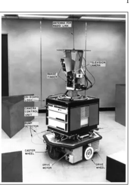
I.2 Shakey the robot . . . 3

I.3 Mobile robot localization scheme . . . 5

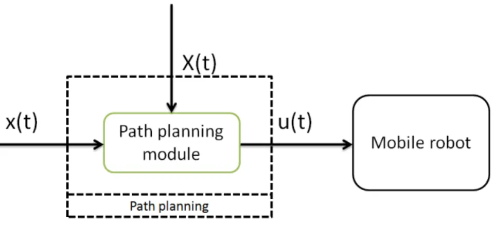
I.4 Path planning scheme . . . 6

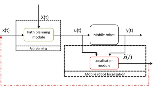
I.5 Path planning + localization scheme . . . 7

I.6 Environment mapping scheme . . . 8

I.7 Localization + Path planning + Mapping scheme . . . 9

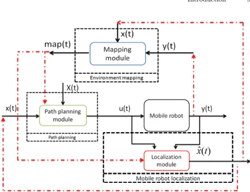
I.8 Localization + Mapping scheme → SLAM scheme . . . 10

1.1 Mobile robot d.o.f. . . 14

1.2 Ultrasonic sensor example . . . 16

1.3 Ultrasonic sensor beam shape . . . 16

1.4 Error in sensor measurement . . . 17

1.5 Incidence angle . . . 17

1.6 Laser rangefinder placed on a mobile robot . . . 18

1.7 Laser rangefinder output example . . . 19

1.8 Mobile robot equipped with a camera . . . 20

1.9 Pinhole model example . . . 20

2.1 Perfectly known rectangular environment . . . 31

2.2 Partially known rectangular environment . . . 33

2.3 Measurement model . . . 34

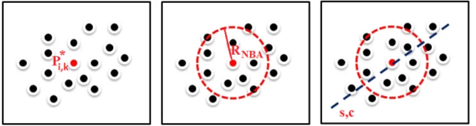
2.4 Properly chosen points Bi (UP), bad chosen points Bi (DOWN) 35 2.5 P∗ i,k approximating the point ˜Pi,k. . . 37

2.6 First picture: P_i,k∗ and previously detected points; second picture: closeness function on P_i,k∗ ; third picture: LMS line approximation . . . 37

2.7 Convex combination based prediction scheme . . . 42

3.1 SLAM main steps . . . 52

(14)

3.3 SLAM second step . . . 53

3.4 SLAM third step . . . 54

3.5 SLAM fourth step . . . 54

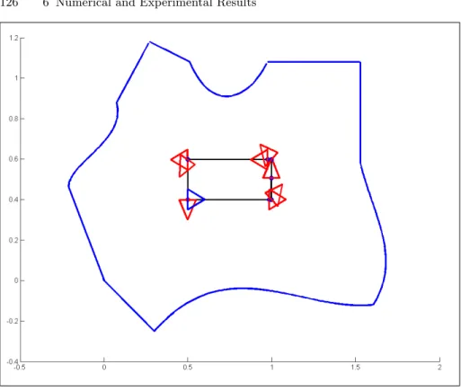
3.6 Real environment (red line), segment based environment boundaries approximation (blue line) . . . 61

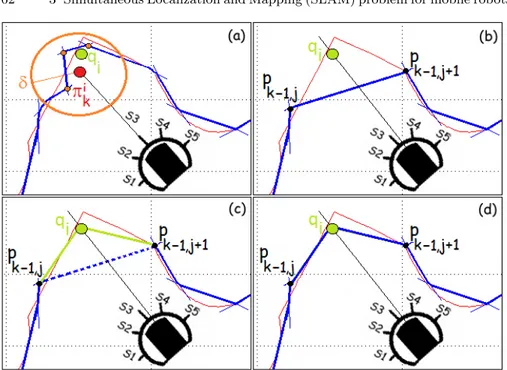
3.7 (a): virtual point qi computation, the orange points and the red point are in Ωi; (b) segment bk−1 computation; (c) and (d): virtual point insertion . . . 62

3.8 Real environment (black line), environment approximating polynomials (light blue line) . . . 67

3.9 An environment boundaries section . . . 74

3.10 Overlapping polynomials . . . 76

4.1 Problems using multiple sensors simultaneously . . . 82

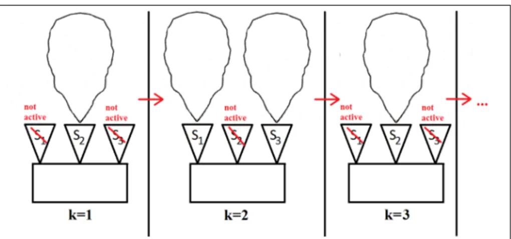
4.2 Sensors beams intersection avoidance thanks to the use of a switching rule . . . 83

5.1 Pinhole model example . . . 92

5.2 Inertial Measurement Unit example . . . 95

5.3 North East Down reference frame . . . 96

5.4 IMU, reference frames and object accelerations . . . 96

5.5 Camera, image and object reference frames . . . 98

5.6 Index εt in some of the performed tests . . . 101

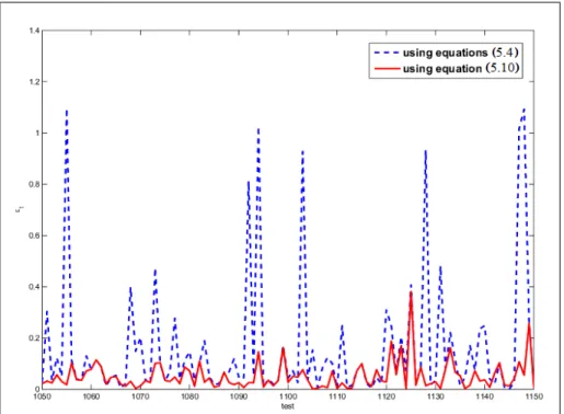
5.7 Index εt minimizing E and minimizing E2 . . . 102

5.8 _{Computation times required to minimize w.r.t. E or w.r.t. E}2 . . 103

5.9 Unit vectors ˆgo and ˆmo . . . 106

5.10 P2P, ∆x= 0 and ∆y = 0 . . . 109

5.11 P2P, ∆x= 0 and ∆y= 0: line unit vector aligned with gravity unit vector . . . 109

5.12 Camera field of view as conic combination . . . 112

6.1 Differential Drive Robot examples . . . 120

6.2 Differential Drive Robot kinematic model . . . 120

6.3 Robot Khepera III equipped with upper body (on the left) and not equipped with upper body (on the right) . . . 123

6.4 Simulative environment: single room. The red triangle represents the robot while the blue circle is robot center coordinates. The black dashed lines are the robot on board distance sensors measurements . . . 124

6.5 Simulative environment: three-rooms. The red triangle represents the robot while the blue circle is robot center coordinates. The black dashed lines are the robot on board distance sensors measurements . . . 124

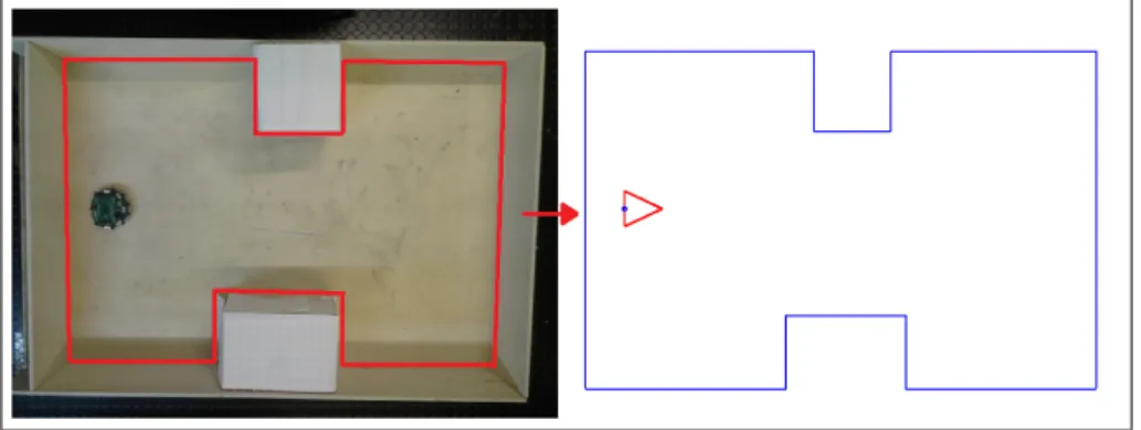
6.6 Experimental environment. The robot Khepera III has been placed into the environment. . . 125

(15)

List of Figures XV

6.7 Experimental environment boundaries . . . 125

6.8 Rectangle trajectory into the single room simulative environment. The blue triangle is robot initial pose . . . 126

6.9 I-like trajectory into the single room simulative environment. The blue triangle is robot initial pose . . . 127

6.10 L-like trajectory into the three-rooms simulative environment. The blue triangle is robot initial pose . . . 128

6.11 Mobile robot on board sensors locations . . . 129

6.12 Real perfectly known rectangular environment . . . 131

6.13 Experimental result using the EKF, rectangle trajectory . . . 132

6.14 Experimental result using the UKF, I-like trajectory . . . 132

6.15 Experimental result using the EKF along with the observations effect maximization switching logic, rectangle trajectory . . . 133

6.16 Experimental result using the UKF along with the Observations effect maximization switching logic, I-like trajectory . . . 134

6.17 Numerical result using the NEKF, rectangle trajectory . . . 135

6.18 Numerical result using the NUKF, I-like trajectory . . . 136

6.19 Experimental result using the NEKF, I-like trajectory . . . 136

6.20 Experimental result using the NUKF, I-like trajectory . . . 136

6.21 Numerical result using the NEKF along with the observations effect maximization switching logic, rectangle trajectory . . . 138

6.22 Numerical result using the NUKF along with the observations effect maximization switching logic, I-like trajectory . . . 138

6.23 Experimental result using the NEKF along with the observations effect maximization switching logic, I-like trajectory . . . 138

6.24 Experimental result using the NUKF along with the observations effect maximization switching logic, I-like trajectory . . . 139

6.25 Standard deviation function estimation . . . 140

6.26 Experimental framework with out of board sensors . . . 142

6.27 MEKF experimental results using Mα= diag{0.1, 0.1, 0.9} . . . 143

6.28 ε, γ, τ evolution changing σ values . . . 145

6.29 SbSLAM simulation result (single room, σ = 0.08) . . . 146

6.30 SbSLAM simulation result (three-rooms, σ = 0.08) . . . 146

6.31 Segment based SLAM results in a real experiment . . . 147

6.32 PbSLAM simulation result (single room) . . . 147

6.33 PbSLAM simulation result (three-rooms) . . . 148

6.34 PbSLAM real result, black line: real environment, green line: estimated environment . . . 148

6.35 EPbSLAM simulation result (single room) . . . 149

6.36 EPbSLAM simulation result (three-rooms) . . . 149

(16)

6.38 Averaged ε index over 300 configurations with n = 4, 5, . . . , 200 feature points . . . 153 6.39 The four squares feature . . . 154 6.40 Pictures taken by the camera in the configuration Rt,1(right)

(17)

List of Tables

6.1 ε index and τ index - perfectly known environment - real

framework experiments . . . 131 6.2 ε index and τ index - perfectly known environment - real

framework experiments . . . 133 6.3 ε index and τ index totally unknown environment

-simulative framework case . . . 134 6.4 ε index and τ index - totally unknown environment - real

framework case . . . 135 6.5 ε index and τ index totally unknown environment

-simulative framework case . . . 137 6.6 ε index and τ index - totally unknown environment - real

framework case . . . 137 6.7 Averaged ε index over the performed 100 experiments . . . 140 6.8 averaged ε index, over the 50 experiments . . . 143 6.9 Averaged indexes over the 100 performed simulations in the

single room environment . . . 144 6.10 Averaged indexes over the 100 performed simulations in the

three-rooms environment . . . 145 6.11 Averaged indexes over the 100 performed simulations in the

single room environment . . . 150 6.12 Averaged indexes over the 100 performed simulations in the

three-rooms environment . . . 150 6.13 Averaged indexes over the 50 performed experiments . . . 151 6.14 Overall results provided by SbSLAM, PbSLAM and EPbSLAM 151

(18)

(19)

Introduction

This thesis focuses on the main theoretical and methodological issues related to the mobile robots navigation. In recent years, due to the continuously increasing use of mobile robots in various applications, all the problems related to this research field have received very considerable attention. Whatever is the mobile robots application goal, the robot has to face three main problems which can be summarized by the following three well known questions: Where the robot is?

Where the robot should go?

How the robot should arrive in its goal location?

This thesis focuses on the first two questions trying to give them a reliable answer. In particular the mobile robots localization problem and the Simultaneous Localization and Mapping (SLAM) problem will be discussed. A set of solutions to both the problems will be proposed in this dissertation. The aim of the thesis is to solve the localization and mapping problems using all the available information in the best possible way and requiring as few a priori assumptions as possible.

History and main topics

A mobile robot is an automatic machine that is capable of movement in a given environment. The history of mobile robots starts in 1939-1945, during the World War II, when the first mobile robots emerged as a result of technical advances on a number of relatively new research fields like computer science and cybernetics. The first mobile robots examples were mostly flying bombs like smart bombs (the V1 and V2 rockets) that only detonate within a certain range of the target using a guiding systems and a radar control.

A second mobile robot example appears in 1948 when W. Grey Walter builds Elmer and Elsie, two autonomous robots called Machina Speculatrix. These robots were able to explore their environment thanks to a very simple

(20)

but efficient strategy: they were both equipped with a light sensor and if they found a light source they would move towards it, avoiding or moving obstacles on their way. These robots demonstrated that complex behaviors could arise from a simple design. The main disadvantage about Elmer and Elsie is related to the light need; the two robots were completely unable to explore dark rooms. Starting from the idea of overcoming this issue, in 1961 the Johns Hopkins University develops Beast, that is a mobile robot which moves around using a sonar to detect its surrounding environment. Thanks to the use of sonar sensors, dark rooms could be explored with no problems. In 1969, Mowbot (see Figure I.1), the first robot that would automatically mow the lawn was developed; it was the first example of mobile robots application in home automation.

Fig. I.1: Mowbot, the first mobile robot in home automation

In 1970 the Stanford Cart line follower was developed, it was a mobile robot able to follow a white line, using a camera to see. It was radio linked to a large mainframe that made the calculations and it represents the first example of the vision based mobile robots. At about the same time, in 1966-1972, the Stanford Research Institute built Shakey the Robot (Figure I.2) a robot named after its jerky motion.

Shakey had a camera, a rangefinder, bump sensors and a radio link. Shakey was the first robot that could reason about its actions. This means that Shakey could be given very general commands, and that the robot would figure out the necessary steps to accomplish the given task. In the same year, the Soviet Union explores the surface of the Moon with Lunokhod 1, a lunar rover repre-senting the first example of mobile robots space application. After six years, in 1976, the NASA sends two unmanned spacecrafts to Mars.

In the 1980s the interest in robots rises, resulting in robots that could be purchased for home use. These robots served entertainment or educa-tional purposes. Examples include the RB5X, which still exists today and the HERO series. Until the ’80s, the robot localization problem and the robot surrounding environment mapping problem have been always faced sepa-rately. During the 1986 IEEE Robotics and Automation Conference, held

(21)

Introduction 3

Fig. I.2: Shakey the robot

in San Francisco, a large number of researches as Peter Cheeseman, Jim Crowley, and Hugh Durrant-Whyte had been looking at simultaneously apply-ing estimation-theoretic methods to both mappapply-ing and localization problems. Over the course of the conference many paper table cloths and napkins were filled with long discussions about consistent mapping. The final result was a recognition that consistent probabilistic mapping was a fundamental problem in robotics with major conceptual and computational issues that needed to be addressed. Over the next few years a number of key papers were produced facing the Simultaneous Localization and Mapping problem (SLAM). The first paper about SLAM was written by Smith and Cheeseman [38], the au-thors describe the SLAM framework and lay down the foundations of SLAM research. After the ’80s, robot navigation received considerable attention by the researchers due to the always increasing interest in mobile robots. In the 1990s Joseph Engelberger, father of the industrial robotic arm, works with colleagues to design the first commercially available autonomous mobile hos-pital robots, sold by Helpmate. In the same year, the US Department of De-fense founds the MDARS-I project, based on the Cybermotion indoor security robot and Andr´e Guignard and Francesco Mondada developed Khepera, an autonomous small mobile robot intended for research activities. In 1993-1994 Dante I and Dante II were developed by Carnegie Mellon University. Both of them were walking robots used to explore live volcanoes. In 1995 the Pioneer programmable mobile robot becomes commercially available at an affordable

(22)

price, enabling a widespread increase in robotics research. In the same years, NASA sends the Mars Pathfinder with its rover Sojourner to Mars. The rover explores the surface, commanded from earth. Sojourner was equipped with a hazard avoidance system which enabled Sojourner to autonomously find its way through unknown martian terrain. In 2002 appears Roomba, a domestic autonomous mobile robot that cleans the floor and in 2003, Axxon Robotics purchases Intellibot, manufacturer of a line of commercial robots that scrub, vacuum, and sweep floors in hospitals, office buildings and other commercial buildings. Floor care robots from Intellibot Robotics LLC operate completely autonomously, mapping their environment and using an array of sensors for navigation and obstacle avoidance. In 2010, the Multi Autonomous Ground-robotic International Challenge has teams of autonomous vehicles which map a large dynamic urban environment, identify and track humans and avoid hostile objects.

Nowadays mobile robots are used in various applications and they are becoming a part of the human life. In particular, robot floor cleaners are available at low prices and many families use them everyday. Robot naviga-tion is becoming one of the most important research field due to the high number of possible applications both in everyday life (home automation) and in research fields (planetary exploration, regions surveillance, rescue missions, ruins exploration).

For any mobile device, whatever is the robot application, the ability to navigate in an environment represents a crucial requirement. Robot naviga-tion means the robot’s ability to determine its own posinaviga-tion in its reference frame (localization) and then to plan a path to a goal location (path plan-ning). Moreover, to navigate in its environment, the robot or any other mobile device requires a representation (a map) of the environment and the ability to interpret this representation (mapping).

Mobile robots localization

The aim of the mobile robots localization problem is to use all the available information, by sensors and by a-priori knowledge on the environment where the robot moves, to localize the robot. This is probably one of the main problems in mobile robotics. To plan a path for a mobile robot or to map the environment surrounding the robot, it is mandatory to known where the robot is or is assumed to be in the environment.

More formally, the problem can be stated as follows:

assume the mobile robot modeled as a set of nonlinear equations ˙

x(t) = f (x(t), u(t))

where x(t) is the robot state, consisting of robot position and orien-tation, and u(t) is a vector containing actuators inputs. Let the robot sensors measurements be modeled as

(23)

Introduction 5

y(t) = h(x(t))

The goal is to obtain a reliable estimation, ˆx(t), of the robot pose (position and orientation) x(t), using all the available information from sensors (y(t)) and actuators (u(t)).

In a schematic point of view, the aim is to develop a localization module able to provide the estimated robot pose starting from the robot inputs and outputs, as shown in Figure I.3.

Fig. I.3: Mobile robot localization scheme

This problem deals with a very big amount of applications. For example, in the cited home automation contexts, the cleaner robots need to localize themselves into the room they have to clean. Thanks to this localization, these robots are able to define which floor parts have been cleaned and which ones have not been visited. Whatever is the application, if an exploration task has to be accomplished then it is required to solve at least the localization problem.

Path planning

Given a mobile robot, modeled as ˙

x(t) = f (x(t), u(t)),

placed in an initial configuration x(ts) = xs, the goal of the path planning

problem is to move the robot from xs to a desired configuration x(tf) = xf

following a desired trajectory χ(t), t ∈ [ts, tf]. More formally, the path

plan-ning strategies aim to find the control moves, u(t), t ∈ [ts, tf] which let the

robot arrive in xf, starting from xs and following as best as possible the

(24)

In a schematic point of view, the aim is to develop a path planning module able to provide the appropriate control moves to the robot, as shown in Figure I.4.

Fig. I.4: Path planning scheme

Obviously, the path planning module needs to know the actual robot pose x(t) and thus the obtained control moves are a function of the desired trajec-tory χ(t) and of the robot pose x(t).

In most applications, the actual robot pose is not directly provided by robot sensors and it has to be obtained through a localization technique. The global scheme can be summarized as shown in Figure I.5. Just to give an example of path planning applications, thinking at planetary exploration tasks, the mobile robots which have to move on an unknown planet have to detect their surrounding environment, they have to localize themselves into this environment and then they have to plan a path to perform in order to explore the region in the most efficient way. Also in this case, whatever is the application, the path planning task has to be accomplished in all the situations concerning regions exploration, navigation or inspection.

Environment mapping

The environment mapping is a task to perform in parallel with the localization task and the path planning task. The aim is to build a robot surrounding environment map as more as possible accurate and reliable. This task can be accomplished in both indoor and outdoor environments and the provided map represents a necessary information to solve the localization problem and the path planning problem.

In particular in all the environments where the GPS can not be used (indoor environment, forests, etc. . . ), if no preliminary assumptions on the

(25)

Introduction 7

Fig. I.5: Path planning + localization scheme

environment structure is done, then the localization task can be accomplished only if the robot builds an environment map ant it localizes itself within this map.

Also for what regards the path planning, to avoid collisions with walls or obstacles, adapting the trajectory χ(t) to the environment, an environment map is required. More formally, the environment mapping problem is the problem of modeling the robot surrounding environment and of estimating its model parameters. In a schematic point of view, a mapping algorithm can be seen as a module which uses the sensors measurements to provide a structure containing all the information required to build the environment map (see Figure I.6).

As shown in Figure I.6, to obtain an environment map, the actual robot pose is needed and, as in the path planning case, a robot pose estimation can be use instead of real robot pose. This estimation is provided by the localization module; the overall scheme is depicted in Figure I.7.

If all the modules in Figure I.7 are correctly developed, than the resulting overall algorithm can be used to answer to the three main questions:

Where the robot is? → localization task and mapping task

Where the robot should go? → localization task and mapping task How the robot should arrive in its goal location? → mapping task and

path planning task

In particular, the loop formed by the localization module, which uses the map provided by the mapping module and from the mapping module, which uses the robot pose estimation to obtain the map, is at the basis of the so

(26)

Fig. I.6: Environment mapping scheme

called Simultaneous Localization and Mapping (SLAM) problem (see Figure I.8).

The mobile robots SLAM problem can be seen as an extension to the localization problem. In the SLAM problem the robot localizes itself into the environment where it moves and it simultaneously builds a map of this environment. In mobile robotics, the SLAM problem is considered as chicken and egg problem due to the very strong correlation between the mapping task and the localization task: the robot, to localize itself within its environment, needs to build a map of this environment but this map can be built only if the robot position is known.

The SLAM problem is probably the mobile robotics topic which finds the bigger amount of applications in various fields. Especially in recent years, mobile robots started to be used in place of humans to accomplish difficult or dangerous tasks. For example:

rescue applications, in which team of mobile robots are used to search and rescue people in disaster regions;

surveillance applications, which regards the use of a single mobile robot or of a team of robots to watch regions of interest;

exploration applications, in which mobile robots are used to build a map of a place in an autonomous way, without any required help by humans.

(27)

Introduction 9

Fig. I.7: Localization + Path planning + Mapping scheme

In all these applications the SLAM problem has to be solved and the resulting performance are completely related to the SLAM algorithm performance.

Personal contribution

The most of the localization, mapping and SLAM techniques proposed in the literature are based on at least some assumptions on the robot surrounding en-vironment and very often this enen-vironment is modeled in a very approximated way. Moreover, all the SLAM algorithms deal with the trade off between local-ization/mapping accuracy and overall algorithm computational cost and the proposed SLAM solutions are usually based on a massive use of the available sensors, neglecting sensors batteries saving.

The aim of the present thesis is to develop a set of localization, mapping and SLAM techniques which have to:

1. be based on very few and weak assumptions on the mobile robot surround-ing environment;

2. provide as accurate as possible localization and mapping results; 3. be fast enough to allow their use in real applications;

4. be as cheap as possible in terms of used sensors (number of sensors and sensors types very influence this point);

(28)

Fig. I.8: Localization + Mapping scheme → SLAM scheme

5. make use of the available sensors in the most possible efficient way in order to save sensors batteries;

6. be developed in a general form in order to allow the use of each technique in various frameworks and using various sensors types.

In this context, a set of new techniques to solve the localization problem, the mapping problem and the SLAM problem, will be described in the follow-ing Chapters. All these solutions have been developed tryfollow-ing, step by step, to accomplish all the previously described goals. In particular, as a first step, some techniques to localize the robot on the basis of a complete knowledge about the robot environment will be shown. As a second step, the required in-formation about the environment will be reduced and a set of solutions based on very weak assumptions on the robot working framework will be proposed. As a final step, these techniques will be improved in order to obtain accept-able computational costs. All the obtained solutions will be tested through numerical simulations and real experiments.

Some of the results presented in the following of this thesis have been published and presented in international journals and during International Conferences. More precisely, regarding the localization problem, it has been faced in [74, 5, 26, 25, 13, 68, 77, 67, 79]; mapping problem solutions and SLAM problem solutions have been shown in [43, 44, 75, 76, 78] .

Thesis overview

(29)

Introduction 11

- Chapter 1 focuses on the mobile robot localization and mapping frame-work description. The mathematical model of a mobile robot moving in a planar environment is described and the most common sensors used to solve the localization and mapping problems are discussed.

- Chapter 2 describes all the developed mobile robots localization tech-niques. Starting from the simpler localization problem in a perfectly known environment, facing then the problem in a partially known environment and, finally, proposing solutions in a completely unknown environment. - Chapter 3 contains an accurate description of all the developed SLAM

solutions. Three main solutions will be shown: a first, very simple, one which is fast in providing mapping and localization results but it yields to approximate environment maps; a second solution which provides an accurate environment description but it requires high computational costs; finally, a third solution, which can be seen as an improvement of the latter two ones, yielding to mapping results as good as the ones obtained using the second technique but with a computational cost as low as the one required by the first technique.

- Chapter 4 focuses on a set of rules and policies to optimally use the available sensors in order to decrease their energy consumptions without affecting their contribution to solve the localization, mapping and SLAM problems.

- Chapter 5 shows a set of alternative mobile robots localization algorithms based on the use of cameras and Inertial Measurement Units. Differently from what is shown in Chapter 1, these techniques are based only on sensors characteristics, they do not use information about the robot model and they have been developed to work only in static context or during very slow robot movements.

- Chapter 6 shows all the numerical simulations and real experiments per-formed to properly test the algorithms described in the first 5 Chapters. Finally, conclusions, showing the achieved goals and describing some possible future investigations, are drawn.

(30)

(31)

1 Localization and Mapping framework

This Chapter focuses on the main features about the framework in which the localization and mapping problems will be solved. The following discussion can be seen as a setup description common to both the second chapter and the third chapter. The mathematical model of a mobile robot moving in a planar environment will be described and the most common sensors used to solve the localization and mapping problems will be discussed.

1.1 Introduction

Starting from the scheme shown in Figure I.7, in this thesis the attention will be paid on the localization and mapping modules design, assuming to be able to properly control the robot. Looking at the literature about localization and mapping problems, many works can be found facing the problem in different ways and using various sensors types.

In particular, the literature shows three main topics about localization and mapping algorithms:

1. used sensors

2. assumptions on the robot surrounding environment 3. algorithms computational cost

In the next Sections, the mobile robot model will be described and a little description about the above three localization and mapping topics will be provided.

1.2 Robot model

In the present thesis, the case of a mobile robot placed in indoor planar envi-ronments will be considered. Once the environment reference frame has been

(32)

chosen, the mobile robot, due to the environment planarity, can be character-ized using only two variables to describe the robot position and one variable to describe the robot orientation. Whatever is the mobile robot type, it has three degree of freedom (d.o.f.), described as depicted in Figure 1.1.

Fig. 1.1: Mobile robot d.o.f.

Let the following notation be used:

Ox1,x2 is the chosen absolute environment reference frame. R is the mobile robot center of gravity.

(xR

1, xR2) are the mobile robot center of gravity coordinates.

θ is the orientation of the robot w.r.t. the x1-axis, considered positive in

counterclockwise.

In mobile robots applications only the robot kinematic model is typically used thanks to the very common assumptions of (1) very slow robot dynamics w.r.t. the robot motor dynamics and (2) very low robot accelerations. The mobile robot motors can thus be considered as static systems and the entire robot dynamics can be neglected. In this context the robot center of gravity R can be denoted as robot center and the mobile robot shown in Figure 1.1 can be described by only three differential equations, one equation for each degree of freedom.

More precisely, the following non linear differential equations can be de-fined    ˙ xR₁(t) = f1(xR1(t), x R 2(t), θ(t), u(t)) ˙ xR₂(t) = f2(xR1(t), x R 2(t), θ(t), u(t)) ˙ θ(t) = fθ(xR1(t), xR2(t), θ(t), u(t)) (1.1)

(33)

1.3 Sensors used in mobile robotics applications 15

where u(t) is an array containing all the robot inputs. Defining the robot state x(t) = [xR

1(t) , xR2(t) , θ(t)]T, the equations (1.1)

are summarized by

˙

x(t) = f (x(t), u(t)). (1.2)

The above equations can be discretized using the Euler forward method [80, 81], obtaining:

xk+1= φ(xk, uk) = xk+ T f (xk, uk) (1.3)

where

T is the sampling period.

xk, uk are the robot state and the robot inputs vector at time tk = kT1.

the function f(·, ·) is the state update function shown in (1.2).

In the following of this thesis, the mobile robot will be always modeled as a set of non linear difference equations affected by noise:

xk+1= φ(xk, uk) + wk (1.4)

where wk= [w1,k, w2,k, wθ,k]T is a Gaussian noise, denoted as process

noise, with zero mean and covariance matrix W . This process noise takes into account unmodeled dynamics, friction, wheels slipping and also, if the case, external disturbances (such as wind).

1.3 Sensors used in mobile robotics applications

The localization and mapping algorithms are very influenced by the used sensors types and the same algorithm can be very efficient using some sensors but it can yield to poor performance using different ones. In the literature, the most popular sensors, used to solve the localization problem and the mapping problem, are ultrasonic sensors, laser sensors and cameras.

1.3.1 Ultrasonic Sensors

Ultrasonic sensors are widely used in many applications thanks to their sim-plicity, availability, and low cost. Such sensors measure (within tolerance) the distance to the surface intercepted by their beam. These sensors are the best sensors for detecting liquids, clear objects, or irregularly shaped objects. They work on a principle similar to radar which evaluate attributes of a target by

1

In the next Chapters and Sections it will be denoted the time step as k ∈ N neglecting the T dependencies. This notation is justified by the isomorphism between the set N and the set of time steps T = {t ∈ R : t = kT & k ∈ N}

(34)

Fig. 1.2: Ultrasonic sensor example

interpreting the echoes from radio waves. Ultrasonic sensors generate high fre-quency sound waves and evaluate the received back echo. Sensors calculate the time interval between sending the signal and receiving the echo to determine the distance to an object. Systems typically use a transducer which generates sound waves in the ultrasonic range, above 18.000 hertz, by turning electrical energy into sound, then, upon receiving the echo, the sensors turn the sound waves into electrical energy which can be measured and displayed.

The sensors achieved performance is very affected by the detected objects surface, material density and material consistency. Moreover, looking at a typical ultrasonic beam shape, depicted in Figure 1.3, a set of troubles related to the use of sonar sensors emerge.

Fig. 1.3: Ultrasonic sensor beam shape

In a nominal point of view, an ultrasonic sensor should measure the dis-tance from an object in front of the sensor. However, due to the sensor beam shape, the obtained measurement can be related to an object which is in the sensor shape but not in front of the sensor itself. This situation is depicted in Figure 1.4

(35)

Fig. 1.4: Error in sensor measurement

If the sensor beam shape was a straight line then the obtained measure-ment would represent the distance d to the object O. However, due to the beam shape, the object O0 could be detected and the obtained measurement will be d0. In this situation the measured distance is d0 while the nominal ex-pected measured distance is d(6= d0), thus the measurement provided by the ultrasonic sensor is erroneous w.r.t the nominal distance.

Moreover also when nofake obstacles (like O0) are in the sensor shape, the measurement provided by an ultrasonic sensor can be erroneous due to sensors physical characteristics. As remarked in [1] and [2], the measurements provided by ultrasonic sensors are really influenced by the incidence angle between the sensor beam and the intercepted surface. Take in consideration the situation shown in Figure 1.5. When the sensor axis is orthogonal to a flat surface, the measurement provided is the true range, within tolerance, to the surface. However, the measurement error can be larger when the beam strikes a surface at a different incidence angle, γ. Consider an ultrasonic sensor, S, which provides the distance, y, from a surface U , as depicted in Figure 1.5.

Fig. 1.5: Incidence angle

Let l(x1, x2) be the tangent line to the surface boundaries in the

intersec-tion point, A, between the incidence surface and the sensor axis. Defining −→y as the sensor axis unit vector and−→b as the l(x1, x2) unit vector, the incidence

angle γ is defined as

(36)

The more the incidence angle is near toπ₂rad, the better the measurement provided by the ultrasonic sensor is.

In conclusion the measurement provided by an ultrasonic sensor can be modeled as a function

y = y(d, γ, v) (1.6)

where

d is the nominal distance from the sensor to the incidence surface of the detected object;

γ is the incidence angle between the incidence surface and the sensor axis; v is a noise used to model the standard measurement error.

Please note that the troublesome situation depicted in Figure 1.4 is modeled using v while the situation shown in Figure 1.5 is modeled using γ. Moreover due to v and γ the obtained measurement y is always y 6= d.

In the literature ultrasonic sensors are widely used to solve the localization problem and the mapping problem. Just a few examples can be found in [32, 31, 33].

1.3.2 Laser sensors

A laser sensor is a device which uses a laser beam to determine the distance to an object. The most common form of laser sensors operates on the time of flight principle by sending a laser pulse in a narrow beam towards the object and measuring the time taken by the pulse to be reflected off the target and returned to the sender.

(37)

A laser rangefinder provides a set of measurements related to the entire sensor surrounding environment, as shown in Figure 1.7. Laser rangefinders can beeasilyused to obtain an environment map and a robot position esti-mation since these sensors provide a large number of measurements and these measurements are very accurate.

Fig. 1.7: Laser rangefinder output example

Regarding the localization and mapping problem using laser sensors, con-crete examples can be found in [6, 40].

1.3.3 Cameras

A camera is a device that records images that may be photographs or moving images such as videos or movies. The term camera comes from the word camera obscura (Latin fordark chamber): an early mechanism for projecting images; the modern camera evolved from the camera obscura.

Cameras may work with the light of the visible spectrum or with other portions of the electromagnetic spectrum. A camera generally consists of an enclosed hollow with an opening (aperture) at one end, for light to enter, and a recording or viewing surface for capturing the light at the other end. A majority of cameras have a lens positioned in front of the camera’s opening to gather the incoming light and focus all or part of the image on the record-ing surface. The diameter of the aperture is often controlled by a diaphragm mechanism, but some cameras have a fixed-size aperture. Most cameras use an electronic image sensor to store photographs on a flash memory. Other cameras, especially the majority of cameras from the 20th century, use pho-tographic film.

It has long been known that a simple pin-hole is able to create a perfect inverted image on the wall of a darkened room, as shown in Figure 1.9.

(38)

Fig. 1.8: Mobile robot equipped with a camera

Fig. 1.9: Pinhole model example

A digital camera is similar in principle; a glass or plastic lens forms an image on the surface of a semiconductor chip with an array of light sensitive devices to convert light to a digital image. The process of image formation, in an eye or in a camera, involves a projection of the 3-dimensional world onto a 2-dimensional surface. The depth information is lost and starting from the image it is not possible to tell whether it is of a large object in the distance or a smaller closer object. This transformation from the 3-dimensional world onto the 2-dimensional one is known as perspective projection and it will be discussed in Chapter 5.

(39)

1.5 Algorithms computational cost 21

About using cameras to solve the localization and mapping problems, ex-amples can be found in [41, 42].

1.4 Assumptions on the robot surrounding environment

For what concerns the assumptions on the robot surrounding environment, most of the previously cited works assume to have at least some information about the environment. For example in [25] and [5] the localization task is accomplished assuming the robot placed in a totally known rectangular en-vironment. In [36] the environment is assumed to be partially known while in [37], the robot is placed in an environment the boundaries of which are assumed to be orthogonal-parallel lines.

As a general rule, the more the assumptions on the robot environment are strong, the simpler will be to solve the localization task and the mapping task.

1.5 Algorithms computational cost

In a computational point of view, it is mandatory for a localization algorithm and for a mapping algorithm to satisfy time constraints since information provided by these algorithms is typically used to compute the output of a control law designed to make the robot follows a given trajectory or completes a given task (see the path planning part in the scheme depicted in Figure I.7). The localization problem when a map of the environment is available has been solved before with efficient algorithms [45, 46]. Similarly, there are well proven and efficient techniques for the generation of environment maps us-ing observations obtained from known locations [47]. However, localizus-ing the robot in a totally unknown environment or simultaneously provide a robot pose estimation and an environment map is a more challenging problem and optimal SLAM approaches, based on Bayesian filtering, could be extremely expensive making them difficult to apply in real time.

In this context, in [44] the proposed robot surrounding environment model is very accurate and versatile but it requires a very high computational effort and, as a consequence, the resulting SLAM algorithm is not feasible in real time applications. On the contrary, the algorithm shown in [43] is based on a more approximate environment model but it is very computationally efficient. As a general rule, the more the provided mapping and localization results are accurate, the higher the computational costs due to these algorithms are.

(40)

(41)

2 Mobile Robots Localization

This Chapter describes a set of new mobile robots localization techniques. Starting from the simpler localization problem in a perfectly known environ-ment, the localization problem will be faced in a partially known environment and, finally, in a completely unknown environment.

2.1 Introduction

The mobile robots localization problem is the problem of localizing a robot within its environment. It finds applications in all the mobile robots con-texts: home automation applications, planetary exploration, rescue missions, surveillance tasks require to know the robot pose (position and orientation). A very few robotics frameworks allow to directly know the robot pose from sensors. For examples, outdoor mobile robotics applications use a GPS but the measurements provided by this sensor are always noisy and very often they are too approximative to be directly used to localize the robot in an accurate way. To overcome this problem, these measurements are fused with other measurements from other sensors to improve the localization results.

In indoor environments, the GPS cannot be used and thus the localiza-tion task has to be solved using other sensors types. In the following, the robot will be assumed to be equipped with distance sensors able to provide measurements about the distance of the robot from the sensors detected ob-jects. These sensors could be, for example, ultrasonic sensors, laser sensors or properly adapted cameras. The goal of this chapter is to find, describe and develop solutions to the Mobile Robots Localization Problem in indoor planar environments. More formally:

given a mobile robot, described by the state equation (1.4) and equipped with a set of distance sensors, the goal is to localize the robot within its environment, providing an estimate of the robot position and ori-entation (robot pose).

(42)

2.2 Proposed Solutions

Robot localization methods can be classified into two main groups [9]: (1) relative positioning methods, and (2) global or absolute positioning methods. The first group (also called dead-reckoning) achieves positioning by odom-etry, which consists of counting the number of robot wheels revolutions to compute the offset relative to a known initial position. Odometry uses the robot model to estimate the robot movements starting from the robot inputs and it is very accurate for small offsets but it is not sufficiently accurate for modeling bigger offsets, because of the unbounded accumulation of errors over time (due to wheel slippage, imprecision in the wheel circumference, or wheel inter axis). Furthermore odometry needs an initial position and fails when the robot is waken-up (after a forced reset for example) or is raised and dropped somewhere, since the reference position is unknown or modified.

Due to the above described reasons, a global positioning system is thus required to recalibrate the robot position periodically. There are essentially two kinds of global positioning systems:

1. techniques based only on the sensors measurements: triangulation or tri-lateration;

2. techniques based on the sensors measurements and on the robot model: Kalman filter based techniques.

Regarding the first family of methods: the triangulation is the geomet-rical process of determining the location of a point by measuring angles to it from known points; the trilateration methods involve the determination of absolute or relative locations of points by distance measurements. Because of the large variety of angle measurement systems, triangulation has emerged as a widely used, robust, accurate, and flexible technique [11]. Various gulation algorithms may be found in the literature [10, 12, 11]; both trian-gulation and trilateration methods yield to the robot position estimation at time tk = kT using only measurements provided at step k. Thanks to this

property, these methods are usually less computationally onerous than the techniques based on sensors measurements and robot model. However due to the lack of knowledge about the measurements history, the triangulation and trilateration techniques may be more affected by measurements noise.

In this thesis, all the proposed mobile robots localization solutions are related to the use of the Kalman filter theory [82, 23]. Unlike triangulation and trilateration methods, the Kalman filter uses the entire available infor-mation on acquired measurements until time tk to obtain the pose estimation

at step k. In particular the Kalman filter theory is widely used in robotics applications, concrete examples can be found in [3, 5, 13].

(43)

2.3 Kalman Filter and its nonlinear extensions 25

2.3 Kalman Filter and its nonlinear extensions

The Kalman filter is an optimal state estimator for a linear model influenced by zero-mean Gaussian noise. Consider the discrete-time linear time-invariant system    xk+1= Axk+ Buk+ wk yk = Cxk+ vk (2.1) where

xk ∈ Rn is the system state vector.

uk ∈ Rmis the system input.

yk∈ Rp is the system output as measured by sensors.

A ∈ Rn×n

, B ∈ Rn×m

, C ∈ Rp×n _{are the system dynamic matrix, input}

matrix and output matrix respectively; more formally, the matrix A de-scribes the dynamics of the system, that is, how the states evolve with time; the matrix B describes how the inputs are coupled to the system states and the matrix C describes how the system states are mapped to the observed outputs.

wk ∼ N (∅, W ) is the process noise and it is a Gaussian noise with

zero-mean and covariance matrix W ∈ Rn×n_{. This Gaussian disturbance takes}

into account for unmodeled dynamics and external disturbances on the state evolution.

vk ∼ N (∅, V ) is the system measurement noise and it is a Gaussian noise

with zero-mean and covariance matrix V ∈ Rp×p. It models the measure-ments noise due to the imperfections in sensors measuremeasure-ments model. vk

and wk are assumed to be statistically uncorrelated.

The general problem that the Kalman filters aims to solve is:

given a model of the system (A, B, C, V, W ), the known inputs uk, k ≤ k,

and the noisy sensors measurements yk, k ≤ k, estimate the state of

the system x_k at step k.

For example, in a robotic localization context, xk is the unknown pose of the

robot, uk contains the commands sent to the robot motors and yk is a vector

containing the measurements provided by robot sensors. The Kalman filter is an optimal estimator for the case where the process and measurement noises are zero-mean Gaussian noises. The filter consists in two main steps. The first step is a prediction of the state based on the previous state and on the inputs that were applied.

ˆ

xk+1|k = Aˆxk|k+ Buk

Pk+1|k= APk|kAT + W

(2.2)

(44)

ˆxk+1|k is the prediction of the state xk+1starting from all the available

information at step k.

ˆxk|k is the estimate of the system state xk, at step k, based on all the

available information at step k.

Pk+1|kis the covariance matrix of the prediction error ek+1|k= xk+1− ˆxk+1|k.

Pk|k is the covariance matrix of the estimation error ek|k= xk− ˆxk|k.

This is an open-loop step and its accuracy depends completely on the quality of the model A and B and on the ability to measure the inputs uk. To improve

the accuracy performance the sensors measurements information is introduced using the so called innovation term

νk+1= yk+1− C ˆxk+1|k (2.3)

which is the difference between what the sensors measure (yk+1) and what

the sensors are predicted to measure (C ˆxk+1|k). A part of this difference will

be due to the noise in the sensors (the measurement noise) but the remain-ing discrepancy indicates that the predicted state was in error and does not properly explain the sensors observations.

At this point, the second step of the Kalman filter, the update step, uses the Kalman gain

Lk+1= Pk+1|kCT(CPk+1|kCT + V )−1 (2.4)

to map the innovation into a correction for the predicted state, optimally tweaking1_{the estimate based on what the sensors have observed. The resulting}

state estimation is ˆ

xk+1|k+1 = ˆxk+1|k+ Lk+1νk+1

Pk+1|k+1 = Pk+1|k− Lk+1CPk+1|k

(2.5)

The term (CPk+1|kCT+ V ) is the estimated covariance of the innovation and

comes from the uncertainty in the state and the measurement noise covari-ance. If the innovation has high uncertainty in relation to some states, this will be reflected in the Kalman gain which will make correspondingly small adjustment to those states.

The above equations constitute the classical Kalman filter which is widely used in applications from aerospace to econometrics. The filter has a number of important properties. Firstly it is recursive, the output of one iteration is the input to the next. Secondly, it is asynchronous: at a particular iteration if no sensors information is available, the prediction step is just performed

1

The Kalman gain is the gain which minimizes the covariance matrix Pk+1|k+1

and it is computed as

Lk+1= arg min Lk+1

(45)

with no update step. In the case that there are different sensors, each with its own C, and different sample rates, the update step is just applied using the appropriate y and C.

The filter must be initialized with a reasonable value of ˆx0|0 and P0|0.

More precisely, ˆx0|0 has to be chosen such that ˆx0|0= E[x0], where E[·] is the

expected value function. The filter also requires the best possible estimates of the covariance of the process and measurement noises (W and V respectively).

2.3.1 The Kalman Predictor

In the literature, as an alternative to the described Kalman filter, there are also works on the use of the so called Kalman Predictor (see [82]) which consists in a simpler algorithm than the standard Kalman filter since it is based only on the prediction step. More formally, while the standard Kalman filter provides the estimate ˆxk|kof the state xk, the Kalman predictor yields

only the prediction ˆxk|k−1 of this state. In a mathematical point of view,

the filter equations are

Kalman Predictor

Lk = APk|k−1CT(CPk|k−1CT + V )−1

ˆ

xk+1|k= Aˆxk|k−1+ Buk+ Lk(yk− C ˆxk|k−1)

Pk+1|k= (A − LkC)Pk|k−1(A − LkC)T + W + LkV Lk

where Pk|k−1is the prediction error covariance matrix related to the prediction

error ek|k−1= xk− ˆxk|k−1.

It has been proved that the Kalman predictor has the same properties of the standard Kalman filter. Obviously, in a computational point of view the predictor is less onerous than the filter since the estimation step is not performed. However due the estimation step loss, the prediction thanks to the Kalman predictor is usually worse than the estimation obtained by the Kalman filter.

2.3.2 Kalman Filter non linear extensions

Now consider the case where the system is not linear and it is described by the equations    xk+1= φ(xk, uk) + wk yk = h(xk) + vk (2.6)

The function φ : Rn_{× R}m _{→ R}n _{describes the new state in terms of the}

previous state and of the system inputs. The function h : Rn _{→ R}p_{maps the}

(46)

At this point, starting from equations (2.6) various extensions to the stan-dard Kalman filter have been developed. In this thesis two of these extensions will be described and used.

The Extended Kalman Filter

The Extended Kalman Filter (EKF) has been used for many years to estimate the state of nonlinear stochastic systems with noisy measurements, and it has been probably the first concrete application of Kalman work on filtering [17]. The filter is based on the linearization of the nonlinear maps (φ, h) of (2.6) around the estimated trajectory, and on the assumption that the initial state and measurement noises are Gaussian and uncorrelated each other. From the computational point of view the EKF is simply a time-varying Kalman filter where the dynamic and output matrices are given by

Ak= ∂φ(x, uk) ∂x _x=ˆ_x k|k , Ck= ∂h(x) ∂x _x=ˆ_x k|k−1 , (2.7)

and its output is a sequence of state estimates ˆxk|k and matrices Pk|k.

Starting from the given (ˆx0|0, P0|0), the Extended Kalman filter steps

are [23]:

Extended Kalman Filter

where ˆxk+1|k represents the estimate of xk+1 before getting the observation

yk+1 (prediction), and ˆxk+1|k+1 represents the estimate after getting that

observation.

In this non-linear context, differently from the linear case, Pk|k is only an

approximation (because of the linearization) of the estimation error covariance matrix.

The Unscented Kalman Filter

The Unscented Kalman Filter (UKF) has been developed to overcome two main problems of the EKF:

(47)

2. the requirement for the noises to be Gaussian [18, 19].

The basic idea behind the UKF is to find a transformation that allows to approximate the mean and covariance of a random vector, of length n, when it is transformed by a nonlinear map. As a first step, a set of 2 n + 1 points, called σ-points, are obtained from the original random vector. As a second step, these σ-points are transformed by the nonlinear map and finally starting from the mean and variance of the transformed σ-points, an approximation of the original random vector mean and variance is obtained. Refer to [19, 20] for the theoretical aspects. Regarding the filter approximating properties, it has been shown [19] that, while the EKF state estimate is accurate to the first order, the UKF estimate is accurate to the third order in the case of Gaussian noises. The covariance estimate also is accurate to the first order for the EKF, and to the second order for the UKF. The so-called NonAugmented version of the Unscented Kalman filter, which is suitable for additive noises, is here reported. The description follows partially the one given in [21], with some modifications to make it more compact and suitable for a MATLAB [22] implementation.

Unscented Kalman Filter – NonAugmented version At each step, starting from ˆx0|0 e P0|0, do

1. Compute Bk|k=p(n + λ)Pk|k, i.e, the scaled square root of matrix Pk|k

2. Compute the σ-points matrix

χk|k= [ˆxk|k xˆk|k+ Bk|k xˆk|k− Bk|k] ∈ Rn×(2n+1)

There (and in the next equations) the sum of a vector plus a matrix is intended as summing the vector to all the column of the matrix (`a la MATLAB)

3. Transform the σ-points matrix (columnwise) χ∗_k+1|k= φ(χk|k, uk)

4. Compute the a-priori statistics ˆ

xk+1|k= χ∗k+1|kR m

Pk+1|k= (χ∗k+1|k− ˆxk+1|k)Rc(χ∗k+1|k− ˆxk+1|k)T+ W

5. Compute the new σ-points

Bk+1|k=p(n + λ)Pk+1|k

(48)

6. Compute the predicted output

Γk+1|k= h(χk+1|k)

ˆ

yk+1|k= Γk+1|kRm

7. Compute the Kalman gain

Pyy= (Γk+1|k− ˆyk+1|k)Rc(Γk+1|k− ˆyk+1|k)T + V

Pxy= (χk+1|k− ˆxk+1|k)Rc(Γk+1|k− ˆyk+1|k)T

Lk+1= PxyPyy−1

8. Compute the a-posteriori statistics ˆ

xk+1|k+1= ˆxk+1|k+ Lk+1(yk+1− ˆyk+1|k)

Pk+1|k+1= Pk+1|k− Lk+1PyyKk+1T

The filter’s parameters and weighs are [18]: Rm_{= [R}m 1 · · · Rm2n+1]T Rc _{= diag{R}c 1, . . . , Rc2n+1} where R1m= λ n + λ, R c 1= λ n + λ+ 1 + β − α 2 Rm j = Rcj = λ 2 (n + λ), j = 2, . . . , 2n + 1. and α = 0.001, β = 2, κ = 3 − n λ = α2_{(n + κ) − n}

According to [18], the choice β = 2 minimizes the error in the fourth-order moment of the a-posteriori covariance when the random vector is Gaussian.

Please note that to use the Unscented Kalman filter no function lin-earization is required. The UKF is then less influenced by model error than the EKF and the estimation provided by the UKF is more accurate than the one obtained using the EKF.

2.4 Mobile robots localization in a perfectly known

environment

In this Section a solution for the mobile robots localization in a perfectly known environment will be proposed. Assume to have a mobile robot placed

(49)

2.4 Mobile robots localization in a perfectly known environment 31

in a rectangular environment the boundaries of which are perfectly known. The robot is assumed to be equipped with nS distance sensors, placed in

known locations w.r.t. the robot center and denoted by Si, i = 1, . . . , nS.

Figure 2.1 shows the described framework for the case nS = 5.

Fig. 2.1: Perfectly known rectangular environment

Assume an absolute reference frame placed in the down-left corner of the rectangular environment. Let lx, ly be the environment width and length

and let αi, i = 1, . . . , 5 denote the orientation of the sensors with respect to

robot axis (orthogonal to wheels axes). The proposed mobile robot localization algorithm is based on the use of an Extended Kalman filter (EKF) or of an Unscented Kalman filter (UKF). The filters are based on the model (1.4) for what regards the robot evolution and, for what concerns the output model, the function h(·) in the equations (2.6) is used. Since the sensors are placed on the robot, the measurements provided by these sensors are related to the environment shape and thus the output equation has to take into account the environment.

Each distance based sensor Si provides the distance of the robot center

from one point on the environment boundaries, denoted by ˜Pi. Starting from

the framework depicted in Figure 2.1 (for the case nS = 5), the distances

yi,k = hi(xk), i = 1, . . . , nS, measured by each distance sensor Si, are given

by hi(xk) = q (tan2_(θ k+ αi) + 1)(xR_1,k)2 if pi ∈ e1, hi(xk) = q (tan2_(θ k+ αi) + 1)(xR1,k− lx)2if pi ∈ e2, hi(xk) = q ( 1 tan2_(θ_k_+α_i₎+ 1)(x R 2,k)2 if pi ∈ e3, hi(xk) = q ( 1 tan2_(θ_k_+α_i₎+ 1)(x R 2,k− ly)2 if pi ∈ e4,

(50)

where ei, i = 1, . . . , 4 denotes the edges of the field, the equations of which

are:

e1: x1= 0; e2: x1= lx

e3: x2= 0; e4: x2= ly

These relationships are specific to the described robot environment and define the robot model output equation. In a more compact form, the above relationships can be written as

yk = h(xk, lx, ly) + vk. (2.8)

As expected, the model output equation is a function of the environment parameters lx, ly and of the robot state xk. The vector vk collects the sensor

noises, also assumed Gaussian, zero-mean, with covariance matrix V , and uncorrelated with the process noise wk.

At this point, using equations (1.4) and (2.8), the Extended Kalman filter and the Unscented Kalman filter presented in Section 2.3.2 can be applied. Thanks to this filter, the robot pose can be estimated and the mobile robots localization problem is solved.

2.5 Mobile robots localization in a partially known

environment

The previously proposed solution can be applied in a few situations due to the very strong assumptions on the environment boundaries. In this section the obtained results for a rectangular environment will be extended to a more general scenario.

Assume that the robot is moving in an unknown workspace and assume to model the environment boundaries using a set of segments, each of them intersecting at least one point on the boundaries (see Figure 2.2).

Let Ox1,x2 be the chosen absolute reference frame and let

{Bi= (B1i, Bi2), i = 1, . . . , nB} be a set of environment boundaries points, the

coordinates of which are assumed to be known. The environment is approx-imated by the segments from Bi to Bi+1, i = 1, . . . , nB and by the segment

starting from BnB and ending in B1

2_{. Consider the same mobile robot used}

in the previous Section. The robot is equipped with nS distance sensors (see

Figure 2.2 for the case nS= 5).

Each sensor provides the distance yibetween the robot center, P = (xR1, xR2),

and one point on the surrounding environment, denoted by ˜Pi= (˜xi1, ˜xi2):

2 _{Please note that if the environment contains obstacles, points on the obstacles}

boundaries are required too. For example, if two obstacles are placed into the environment, three points sets have to be used: the first one related to the envi-ronment, the second one and the third one related to the obstacles. Only segments related to points in the same set are used.

(51)

2.5 Mobile robots localization in a partially known environment 33

Fig. 2.2: Partially known rectangular environment

yi=

q (xR

1 − ˜xi1)2+ (x2R− ˜xi2)2. (2.9)

The above measurement is approximated by the distance between P and the intersection point, ¯Pi = (¯xi1, ¯x

i

2), between the Si sensor axis and one of

the segments used to model the boundaries (see Figure 2.3).

Denoting the Si sensor axis by x2 = aix1+ qi, and the detected segment

axis by x2= cix1+ si, the intersection ¯Pi is

¯ xi1= si− qi ai− ci , x¯i2= aisi− ciqi ai− ci . (2.10)

Finally the distance between P and ˜Pi is approximated by:

ηi= q (xR 1 − ¯xii)2+ (x R 2 − ¯xi2)2≈ yi. (2.11)

Figure 2.3 shows in details the proposed observation model for the case Si= S3.

The Si axis parameters are given by:

ai= tan(θ + αi), qi= xR2 − aixR1, (2.12)

where θ is the robot heading. Using (2.10) and (2.12) within (2.11), a distance function ηidepending only on the robot state and on the segment parameters,

(si, ci), can be obtained

ηi= h((xR1, x R

2, θ), (si, ci)), i = 1, . . . , nS.

These relationships allow to define the robot model output equation: