Verifica e validazione preliminare sull’accoppiamento del codice di calcolo RELAP5/Mod.3.3 e il codice di fluidodinamica computazionale ANSYS Fluent

(1)

(2)

CIRTEN

Consorzio Interuniversitario per la Ricerca TEcnologica Nucleare

Lavoro svolto in esecuzione dell’Attività LP2. C1

AdP MSE-ENEA sulla Ricerca di Sistema Elettrico - Piano Annuale di Realizzazione 2014 Progetto B.3.1 “Sviluppo competenze scientifiche nel campo della sicurezza nucleare e collaborazione ai

programmi internazionali per il nucleare di IV generazione”

UNIVERSITÀ DI PISA

Preliminary verification and validation of coupled

calculation between the RELAP5/Mod. 3.3 STH code

and the CFD code ANSYS Fluent

(Verifica e validazione preliminare sull’accoppiamento

del codice di calcolo RELAP5/Mod. 3.3 e il codice di

fluidodinamica computazionale ANSYS Fluent)

Autori

F. Andreoli, G. Damiani, D. Martelli, N. Forgione, W. Ambrosini

CERSE-UNIPI RL 1545/2015

(3)

1

Summary

The aim of the present work, carried out at DICI of University of Pisa, is to contribute to the development and improvement of coupling methods between CFD codes and thermal-hydraulic system (STH) codes.

The CFD solvers adopted are STAR-CCM+ and Fluent, whereas only the system code RELAP5 is used. The work was structured in two parts.

The first part aims at simulating with STAR-CCM+ the Protected Loss Of Heat Sink (PLOHS) with Loss Of Flow (LOF) accidental scenario inside CIRCE pool type facility with DHR. For this purpose, two different simulations have been considered. In the first one, the boundary conditions imposed in STAR-CCM+ are extracted from CIRCE Test I experimental data. In the second one, the boundary conditions applied in the CFD code are taken from RELAP5 calculations. In this way, a “one-way” coupling methodology was applied between STAR-CCM+ and RELAP5. Preliminary calculations have been carried out in order to verify the correct implementation of such boundary conditions into STAR-CCM+ and to obtain an initial verification of the capability of the CFD solver to reproduce a thermally stratified flow. A good agreement was found between the obtained results and a previous work dealing with a “one-way” coupling methodology between Fluent and RELAP5.

The second part deals with the development of a “two way” implicit coupling scheme between Fluent and RELAP5 in order to simulate a CIRCE experimental test representative of an isothermal gas enhanced circulation test. In order to simulate the cover gas in the LBE pool of the facility, the VOF (Volume Of Fluid) model of Fluent has been used. Moreover, the computational efforts has been successfully enhanced by the use of a new methodology for interact with the Fluent code. The performed simulations are the first application of the in-house developed coupling tool for a pool type facility, showing the opportunity to determinate a new data exchange methodology in order to guarantee a proper convergence. The obtained results shows good agreement with the experimental data giving confidence on the developed tool.

(4)

2

Index

Summary ... 1 Index... 2 List of figures ... 3 List of Tables ... 4 1. Introduction ... 5

2. Circe experimental facility and ICE test section ... 6

2.1. CIRCE facility ... 6

2.2. ICE test section ... 6

2.3. Decay Heat Removal heat exchanger ... 7

3. STAR-CCM+ simulations of PHLOS+LOF inside CIRCE facility ... 9

3.1. CIRCE Test I experiment ... 9

3.2. CFD computational domain and numerical model ... 10

3.3. Boundary conditions... 12

3.3.1. Test I ... 12

3.3.2. RELAP5 calculation ... 13

3.4. Results of preliminary simulations ... 14

3.4.1. Comparison with Test I ... 14

3.4.2. Comparison with RELAP5/Fluent coupled simulations ... 18

4. Development of a Coupled RELAP5-Fluent Model ... 21

4.1. Computational Domains and Mathematical Models ... 21

4.1.1. RELAP5 Stand-Alone nodalization ... 21

4.1.2. Discretization of the coupled system ... 23

4.1.3. VOF model ... 30

4.2. Coupling procedure and strategies ... 31

4.2.1. Implicit coupling scheme ... 33

4.2.2. Improvements of the new coupled code ... 34

4.3. Simulation Tests ... 35

4.4. Obtained results ... 37

5. Conclusions ... 41

(5)

3

List of figures

Figure 1: CIRCE experimental facility ... 6

Figure 2: ICE test section ... 8

Figure 3: LBE flow rate through ... 10

the primary system during Test I ... 10

Figure 4: Thermal power removed by the HX during Test I ... 10

Figure 5: Average temperatures through the FPS during Test I ... 10

Figure 6: 2D axial-symmetric domain. [9] ... 11

Figure 7: Polyhedral mesh used for preliminary tests... 11

Figure 8: Boundary conditions for the LBE (left) and air (right) [9] ... 12

Figure 9: Power decrease trend ... 13

applied in the HX ... 13

Figure 10: LBE mass flow rate trend ... 13

imposed at the entrance of the HS ... 13

Figure 11: LBE mass flow rate trend ... 13

imposed at the entrance of the HS ... 13

Figure 12: Power decrease trend ... 13

applied in the HX ... 13

Figure 13: Distribution of temperature in the domain at t = 0 h (left) and t = 30 h (right) ... 15

Figure 14: Temperature through the HS ... 15

Figure 15: Temperature through the HX in the present work (a) and in CIRCE ((b)  Tin, (c)  Tout) ... 16

Figure 16: Control line at y = 0.3 m in the LBE pool region [9] ... 16

Figure 17: Temperature profile along the vertical control line (y = 0.3 m) ... 17

Figure 18: Thermal power removed by the DHR in the present work (left) and in CIRCE (right) ... 17

Figure 19: DHR LBE mass flow rate in the present work (left) and in CIRCE (right) ... 18

Figure 20: Air temperature distribution along two vertical control lines after 30 h ... 18

Figure 21: DHR LBE mass flow rate: present work (left) Fluent calculations (right) ... 19

Figure 22: Thermal power removed by the DHR: present work (left) Fluent calculations (right) .... 19

Figure 23: Air temperature distribution along two vertical control lines after 20 h: ... 19

present work (left) Fluent calculations (right) ... 19

Figure 24: Temperature profile along the vertical control line (y = 0.3 m): ... 20

Figure 25: Temperature time trends at the outlet of the HX and at the inlet of the HS: ... 20

Figure 26: RELAP5 Stand – Alone nodalization of CIRCE facility ... 22

Figure 27: Geometry decomposition of the domain [9] ... 23

Figure 28: RELAP5 part for coupled simulation – ICE + HX... 24

Figure 29: CFD domain – Pool + DHR ... 25

Figure 30: Coarse mesh details (“standard wall function”) ... 27

(6)

4

Table 1: meshes parameters ... 28

Figure 32: LBE temperature comparison between the two meshes ... 29

Figure 33: LBE Volume fraction initialization for the VOF model ... 31

Figure 34: Nodalization and exchanged variables for the RELAP5 – Fluent coupled model ... 32

Figure 35: Implicit coupling scheme ... 34

Figure 36: New coupled code scheme ... 35

Table 2: Forced circulation test ... 36

Figure 37: Argon mass flow rate – Input data for simulations ... 36

Table 3: Matrix of performed simulations ... 36

Figure 38: LBE mass flow rate time trend ... 37

Figure 39: ICE Inlet and Outlet LBE mass flow rate for coupled simulations Step 2 ... 38

Figure 40: ICE Inlet and Outlet pressure for coupled simulations Step 2 ... 38

Figure 41: Separator and pool LBE height level ... 39

Figure 42: LBE mass flow rate for coupled simulation Step 4 ... 39

Figure 43: LBE mass flow rate for coupled simulation Step 6 ... 40

Figure 44: Experimental vs calculated LBE mass flow rate ... 41

for RELAP5 stand – alone and coupled simulations ... 41

List of Tables

Table 1: meshes parameters ... 28

Table 2: Forced circulation test ... 36

(7)

5

1. Introduction

The computational analysis of a large pool system during operational and accidental transient using System Thermal Hydraulic codes (STH) is generally inadequate. Phenomena as mixing, thermal stratification, recirculation and dissipating flows can influence the fluid dynamic involved during the transient. STH codes are indeed based on partially differential equation for two-phase flow and heat transfer (mass, momentum and energy) usually solved by finite-difference methods based on one dimensional approximation. In some STH codes as RELAP5-3D and CHATARE, a three dimensional model has been implemented with limitations on nodalizations, field equations and physical models (e.g. lack of turbulence modelling). However, for such analysis, the exclusive use of a Computational Fluid Dynamic code (CFD) still remain prohibitive for the computational efforts required even using simplified domain and Porous medium approach for the simulation of reactor cores and heat exchangers where the minimum spatial resolution of the mesh is fixed by sub-channel size. Therefore, the coupling between STH and CFD codes seems to be at present a promising technique to study complex and large system where different range of scale phenomena take place. With this methodology, the computational domain is subdivided into two or more parts that are simulated by the different codes. The interfaces between the parts of the domain constitutes the boundary condition where the data exchange between the two codes occur.

In 2012 at the DICI (Dipartimento di Ingegneria Civile e Industriale) of the University of Pisa, a first application to a simplified representation of NACIE facility of an in-house developed coupling tool between the RELAP5/Mod.3.3 thermal-hydraulic system code and the CFD Fluent commercial code was performed. A comparative analysis of the simulations performed by RELAP5-Fluent coupled codes and by RELAP5 stand-alone code showed good agreement among them [1]. In 2013 the coupling tool was improved modifying the correlations used by the RELAP5/Mod.3.3 system code to obtain the thermodynamic properties of lead, LBE and sodium in agreement with Sobolev work [2], [3]. Moreover, the obtained results of the RELAP5 stand-alone and RELAP5-Fluent coupled simulations were compared with the data coming from the experimental campaign performed on the NACIE facility.

In 2014 new developments and improvements dealing with the coupling technique were performed. In particular, a new implicit numerical scheme was developed, then both the explicit and implicit coupling tool have been parallelized in order to perform multi processor CFD calculations inside the coupled model (RELAP5 calculations are performed with single processors). For the description of the coupling tool in the explicit coupled version and for the description of the NACIE facility see [1] and [3]. For the improved coupling tool in the implicit version see Ref. [4].

Finally, in this work a new coupled model between the CFD code Fluent and the STH code RELAP5 has been developed for a pool type facility configuration (CIRCE). In particular, a test of gas enhanced circulation is investigated and a new “two way” implicit numerical scheme together with a new coupling methodology are developed. Moreover, “one-way” coupled simulations with the CFD solver STAR-CCM+ have been carried out investigating a PLOHS+LOF accidental scenario inside CIRCE facility.

(8)

6

2. Circe experimental facility and ICE test section

2.1. CIRCE facility

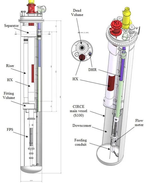
In the frame of the THINS EU Project, a large-scale integral test named “CIRCE experiment” (CIRCulation Experiment) was implemented and carried out at the Brasimone-ENEA Research Centre. The experiment aimed at analysing mixed convection heat transfer and thermal stratification in a heavy liquid metal pool during the transition from forced convection (nominal conditions) to natural circulation.

The CIRCE facility consists of a main cylindrical vessel (S100) filled with about 70 tons of molten Lead-Bismuth Eutectic (LBE) as coolant fluid and argon is the cover gas. The facility also contains a LBE storage tank (S200), a small LBE transfer tank (S300) and the data acquisition system (see Figure 1) [5]. The experiment was performed on the test section named “Integral Circulation Experiment” (ICE), described in the next section.

Figure 1: CIRCE experimental facility

2.2. ICE test section

The Integral Circulation Experiment (ICE) test section is placed into the S100 main vessel and was realized with the aim of reproducing thermal-hydraulic behaviour of the Experimental Accelerator Driven System (XT-ADS) and European Facility for Industrial Transmutation (EFIT) primary system [6] [7] [8]. It consists of the following components (see Figure 2):

Downcomer: it is the volume between the test section and the main vessel, which allows the

hydrodynamic connection between the outlet section of the heat exchanger (HX) and the inlet section of the feeding conduit.

(9)

7

Fuel Pin Simulator (FPS): it is a mechanical structure that simulates the core of the reactor,

representing the Heat Source (HS) of the system. It is connected in the lower section to the flow meter and in the upper section to the insulation volume. In the upper section, the FPS is hydraulically linked to the fitting volume, ensuring continuity of the main flow path.

Fitting Volume: it is placed in the middle part of the test section, and allows the hydraulic

connection between the HS and the riser.

Riser: it is an insulated pipe (double wall pipe with air in the gap) connecting the fitting

volume with the separator. A nozzle is installed in the lower section to allow the argon injection inside this pipe (forced circulation is assured by a gas-lift technique).

Separator: it is a volume that connects the riser with the HX. It allows the separation of the

LBE flowing downward into the HX from the Argon flowing in the test section cover gas through the free surface. In addition it allows fluid expansion during transient operations.

Heat Exchanger:it corresponds to the heat sink of the system. It consists of double-wall

bayonet tubes (with helium gap) fed by low pressure boiling water. Its thermal duty is 800 kW. In order to promote natural circulation along the primary flow path, it is installed in the upper part of the test section.

Dead Volume: it consists of two concentric pipes. The inner pipe is connected, by bolted

junctions, to the FPS (by the coupling flange) and to the cover head. The volume inside the inner pipe is named Insulation Volume. The outer pipe is welded to the inner pipe in the lower end by a flange, which allows a bolted connection between the dead volume and the fitting volume. It extends to the cover gas, above the free level. The annulus between the inner and outer pipes is linked to the cover gas and filled by a thermal insulator.

Decay Heat Removal System: it represents the heat sink of the system in the case of DHR

scenario, when the HX is unavailable. It is hydraulically de-coupled by the primary system being placed into the downcomer. The DHR heat exchanger is designed to have a thermal duty of 40 kW, which represents 5% of the ICE nominal power (800 kW). It is briefly described in the following section.

2.3. Decay Heat Removal heat exchanger

The DHR heat exchanger is placed in the upper part of the pool reactor and works in natural circulation on the primary LBE side and in forced circulation on the secondary air side; it is activated following an accidental event with total loss of secondary circuit and consequent reactor scram.

The position of the DHR in the CIRCE facility is shown in Figure 2. The DHR is essentially a heat exchanger made of three concentric tubes, of which the intermediate has a bottom end sealed, while the internal and external tubes are opened at the bottom.

In the inner tube, the cold air at atmospheric pressure is injected from the top, flows downward and then upward in the annulus between the inner and intermediate tubes. In the annulus, the air increases its energy removing heat from the LBE, realizing a counter current heat exchange. The LBE enters the DHR from the top through appropriate holes, and then it flows downward into the annulus between the intermediate and external tubes.

(10)

8

In order to thermally insulate the LBE flowing in the DHR annular pipe from the LBE pool, a gap of air is present on the DHR outer shell. In particular, thermal insulation is realized by a double wall with a gap of 4.6 mm filled by air at room pressure and temperature (before the sealing) and this device allows a drastic reduction of the thermal coupling with the downcomer.

A more detailed description can be found in Ref. [5].

(11)

9

3. STAR-CCM+ simulations of PHLOS+LOF inside CIRCE facility

Thermal fluid-dynamics analyses for a Protected Loss of Heat Sink (PLOHS) with Loss of Flow (LOF) accidental scenario inside the CIRCE facility are performed with the CFD solver STAR-CCM+. In particular, the transition from forced to natural circulation is investigated together with the thermal stratification inside the CIRCE pool. For this purpose, two different URANS simulations have been carried out. In the first one, the boundary conditions imposed into the CFD code are extracted from experimental data (CIRCE “Test I” experiment [9]). Whereas, in the second one, a “one-way” coupling methodology between STAR-CCM+ and the thermal-hydraulic system code RELAP5 is developed, i.e. the boundary conditions imposed in STAR-CCM+ are obtained from a previous calculation performed with RELAP5 [5].

This Section is structured as follows. CIRCE “Test I” experiment is briefly described in Section 3.1. The computational domain, mesh and numerical method are presented in Section 3.2. The CFD boundary conditions extracted from Test I and from RELAP5 calculation are reported in Sections 3.3.1 and 3.3.2, respectively. Preliminary simulations have been performed in order to verify the correct implementation of boundary conditions into STAR-CCM+ and results are presented in Section 3.4.

3.1. CIRCE Test I experiment

The “Test I” experiment performed in the CIRCE facility, reproduces a PLOHS+LOF accidental scenario. This accident is characterized by the total loss of the secondary circuit with consequent reactor scram and activation of DHR system to remove the decay heat power (5-7% of the nominal value). In the CIRCE-ICE facility, the transition from forced circulation (at nominal conditions) to natural circulation is obtained reducing the thermal power generated in the HS, stopping the argon injection into the riser, cutting off the main HX, and activating the DHR heat exchanger.

Test I starts with a nominal power of about 730 kW, and after roughly 7 hours the transition to 50 kW takes place. The primary LBE flow rate, under forced circulation conditions, reaches a nominal value of about 56-57 kg/s, as shown in Figure 3. After the gas injection switches off and the electrical power supply reduces to about 5% of nominal power, natural circulation establishes. LBE flow rate tends to about 7.5 kg/s (14% of the nominal flow rate). Meanwhile, the HX power reduces to about zero, as shown in Figure 4, and the DHR-system is activated. The air mass flow rate through the DHR is about 0.223 kg/s.

Figure 5 displays the average temperatures at inlet and outlet sections of the FPS. Steady state temperatures at nominal power are reached after 4-5 hours of transient assuming values of 285 and 362°C for inlet and outlet sections, respectively. After the transient initiation, the average temperature at the FPS outlet decreases by 70°C, reaching a value of about 295°C, while the average temperature at the inlet section decreases by 5°C to a value of about 280°C. Then, natural circulation establishes with a temperature difference of about 24°C. Figure 5 clearly shows that after a transient of about 40 hours, the average temperature in the FPS still increases because the air mass flow rate in the DHR is not sufficient to remove the power produced in the FPS.

(12)

10 Figure 3: LBE flow rate through

the primary system during Test I

Figure 4: Thermal power removed by the HX during Test I

Figure 5: Average temperatures through the FPS during Test I

3.2. CFD computational domain and numerical model

In the present work, due to the huge size of the CIRCE facility main vessel and the long duration of the simulated transient, a simplified 2D domain configuration is considered with the aim of reducing the computational power required. In more detail, a 2D axial-symmetric geometry has been designed with the DHR axis as axis of symmetry (Figure 6). In order to facilitate the CFD requirements, some simplifications have been introduced. For instance, only the DHR and the LBE pool inside the mail vessel are completely reproduced, while other components of ICE test section, such as HS, Riser, gas separator and HX, are schematically represented. In particular, these components have been modelled maintaining the same transit time of the real geometry and the same heat flux in the HS and HX. The LBE pool has been designed maintaining the same cross sectional area of the CIRCE LBE pool at the same vertical position.

The computational domain has been discretized using polyhedral cells with prism layers next to the walls in order to resolve the viscous effects on the wall. This mesh is created using a Parts-Based Meshing technique and the Automated Mesh (2D) operation [10].

0 5 10 15 20 25 30 35 40 45 50 0 10 20 30 40 50 60 70 Mm (LBE) L B E F lo w R a te [k g /s ] Time [h] 0 5 10 15 20 25 30 35 40 45 50 -200 -100 0 100 200 300 400 500 600 700 800 Q(HX) T h e rm a l p o w e r [k W] Time [h] 0 5 10 15 20 25 30 35 40 45 50 280 300 320 340 360 380 400 420 A v e ra g e t e m p e ra tu re [ °C ] Time [h] Average T_in Average T out

(13)

11

As already said, a long transient has to be simulated; therefore, preliminary calculations with a coarse mesh have been carried out in order to verify the correct implementation of boundary conditions into STAR-CCM+. Such mesh consists of about 128000 polyhedral cells, and it is shown in Figure 7. By using this mesh, reasonably good information about the main trend of the flow during the transient can be obtained in a short computational time. Therefore, it is useful in order to have an initial check of the capabilities of STAR-CCM+ to reproduce thermal stratification inside CIRCE pool. The adopted turbulence model is the SST k-ω model by Menter, which is an improved version of the original standard k-ω model developed by Wilcox, and the all y+ wall treatment has been used [10].

Figure 6: 2D axial-symmetric domain. [9] Figure 7: Polyhedral mesh used for preliminary tests

The LBE properties, such as density, molecular viscosity, thermal conductivity and specific heat, are assumed as a function of the temperature (in [K]) in agreement with the Handbook on Lead-bismuth Eutectic Alloy and Lead Properties, Material Compatibility, Thermal-hydraulics and Technologies, 2007 [11]. Constant properties are considered for the air [12].

For both the computations performed, an initial steady state calculation assuming nominal operating conditions has been performed (all residuals are below 1.0E-7). Then, transient calculations, reproducing the transition from forced to natural circulations, have been carried out. The unsteady implicit time integration scheme is used with 1st order temporal discretization and a time step of 1 s.

DHR HX FPS HX RiserFPS DHR

S100

Geometrical Domain

(14)

12

3.3. Boundary conditions

In order to reproduce the LBE flow path inside the CIRCE facility, a mass flow inlet has been set at the HS entrance, whereas a pressure outlet is assumed at the domain exit, see Figure 8. Positive and negative thermal powers are imposed at the walls of the HS and HX, respectively. For simplicity, the external walls of the pool are set as adiabatic and no-slip conditions are assumed. Moreover, gravity along the x-axis is considered. A mass flow inlet and a pressure outlet are imposed at the air in the secondary circuit of the DHR, as shown in Figure 8. The next two sections highlight the boundary conditions extracted from Test I experimental data and RELAP5 calculation and imposed into STAR-CCM+.

Figure 8: Boundary conditions for the LBE (left) and air (right) [9]

3.3.1. Test I

In the initial steady state calculation, a nominal power of 730 kW in the HS and an equal power removed by the HX are imposed. Moreover, the mass flow rate and the temperature at the HS inlet are 56 kg/s and 285°C, respectively. Since the DHR is not yet activated, a wall boundary condition is imposed at the inlet and outlet sections of the secondary circuit of the DHR.

During the transient, the HS power is reduced to 50 kW. The heat power removed by the HX decreases to zero in about half an hour. The decrease trend has been set by means of a field function imposing the heat flux time trend reported in Figure 9. The mass flow rate at the entrance of the HS decreases to about 7.5 kg/s, and the decrease trend, shown in Figure 10, has been set by means of a field function. Another field function has been implemented in order to evaluate the LBE average temperature at the exit of the domain and set as LBE temperature at the entrance of the HS. In the DHR, the inlet air mass flow rate and temperature are set to 0.223 kg/s and 20°C, respectively.

Mass flow inlet Pressure outlet HS x y Air LBE LBE

(15)

13 Figure 9: Power decrease trend

applied in the HX Figure 10: LBE mass flow rate trend imposed at the entrance of the HS

3.3.2. RELAP5 calculation

The boundary conditions obtained from RELAP5 calculation are slightly different from Test I. During the initial steady state simulation, the nominal power in the HS (and removed by the HX) is 800 kW. The LBE mass flow rate at the entrance of the HS is 54.8 kg/s and a temperature of about 300°C is set at the entrance of the HS. Then, a transient of about 20 hours is initiated. The LBE mass flow rate and the HX power decrease trends, shown in Figure 11 and Figure 12, are imposed by means of field functions. The LBE average temperature at the exit of the domain is monitored and set as LBE temperature at the entrance of the HS by means of a field function. The HS power is reduced to 40 kW and the DHR is activated with an air mass flow rate of 0.3 kg/s and an inlet temperature of 20°C.

Figure 11: LBE mass flow rate trend imposed at the entrance of the HS

Figure 12: Power decrease trend applied in the HX

(16)

14

3.4. Results of preliminary simulations

3.4.1. Comparison with Test I

The initial steady state is characterized by a forced convection regime. The LBE enters the HS at 285°C; it heats up and flows upward through the Riser. From the Riser exit, LBE flows through the Separator into the HX shell. There, it cools down and flows downward into the pool. Inside the pool, the temperature is uniform at about 285°C, as reported in Figure 13.

Figure 14 displays the average temperatures at inlet and outlet sections of the HS. At time 0 h, corresponding to the two circles in the figure, the temperatures are about 285°C and 375°C for inlet and outlet sections, respectively. This is in accordance with the relation ∆𝑇 = 𝑄/(𝑚̇𝑐_𝑝), being Q the thermal power, 𝑚̇ the mass flow rate, and cp the specific heat. In fact, for the boundary

conditions specified in Section 3.3.1, and a cp of approximately 144 kJ/(kgK), a ∆𝑇 = 90°C is

obtained. In CIRCE (Figure 5), the outlet temperature in the HS is slightly lower (362°C), mostly due to the heat losses towards the external environment and the fact that part of the supplied electrical power is converted into heat in the electrical cable for Joule effect.

From these steady state conditions, the transition from forced to natural circulation is initiated and a total of 30 hours is investigated. The sharp reduction in the HS thermal power, the non-instantaneous reduction in the thermal power removed by the HX, and the activation of the DHR, cause a rapid decrease in the HS outlet temperature to about 291°C, and a more slowly decrease in the HS inlet temperature to about 272°C, as displayed in Figure 14. Then, temperatures start to increase due to the reduced mass flow rate and to the loss of cooling from the HX. After about 3 hours, natural circulation establishes, and the temperature difference in the HS falls from 90 to about 46.8°C. Again, such ΔT can be easily confirmed by using the aforementioned relation with the new boundary conditions.

By comparing Figure 14 with Figure 5 (from CIRCE), it can be noted that the code calculation correctly reproduces the time trend of temperature obtained in CIRCE; however, some differences are present. For instance, at the beginning of the transient, the HS inlet temperature reaches a lower value and for a longer time than in CIRCE, thus, affecting the outlet temperature trend. Moreover, at natural circulation conditions, temperatures increase faster. In particular, it can be seen that inlet and outlet temperatures at 30 h are about 417°C and 464°C; much higher than 349°C and 373°C obtained in CIRCE at the end of the experiment. These differences are related to the absence of structures inside the pool and from the assumption of adiabatic walls in the code calculation. Moreover, the effects of a coarse discretization could play an important role in this deviation from the experimental results. Therefore, additional investigations with a finer mesh are handy in order to isolate the physical effects from the numerical ones.

(17)

15

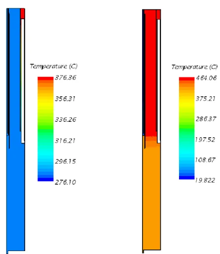
Figure 13: Distribution of temperature in the domain at t = 0 h (left) and t = 30 h (right)

Figure 15 compares the obtained trends of temperature over time at the inlet and outlet sections of HX (Figure 15 a) with the experimental data (Figure 15 b, c). As already noticed for the HS, the trend is qualitatively reproduced with the aforementioned differences. Moreover, it can be seen that, at natural circulation flow regime, there is no difference between inlet and outlet temperatures due to the adiabatic condition imposed at the walls. On the contrary, the experiment shows ΔT = 4-5°C.

(18)

16

(a)

(b) (c)

Figure 15: Temperature through the HX in the present work (a) and in CIRCE ((b)  Tin, (c)  Tout)

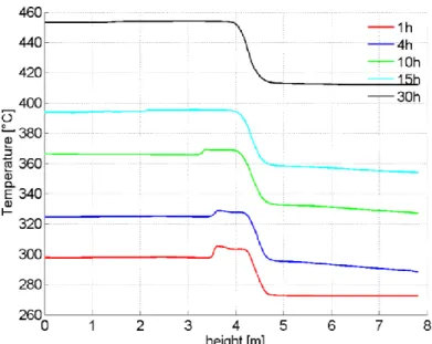
As in the RELAP5/Fluent coupled simulations [9], a vertical control line placed al y = 0.3 m (Figure 16) is used in order to monitor the temperature profile in the LBE pool region, and temperature trends along this line are given in Figure 17. Computational analysis confirms that the temperature gradient is restricted to a well-defined region between the HX and the DHR, as shown also in Figure 13. The temperature difference between the upper “hot” region and the lower “cold” region is about 40°C.

Figure 16: Control line at y = 0.3 m in the LBE pool region [9]

0 5 10 15 20 25 30 35 40 45 50 300 310 320 330 340 350 360 370 380 390 T e m p e ra tu re [ °C ] Time [h] T In SG T-SG-01 T-SG-02 T-SG-03 T-SG_IN,av 0 5 10 15 20 25 30 35 40 45 50 240 260 280 300 320 340 360 380 T e m p e ra tu re [ °C ] Time [h] T Out SG T-SG-13 T-SG-14 T-SG-15 T-SG-16 T-SG-17 T-SG-18 T-SG_OUT,av g

(19)

17

Figure 17: Temperature profile along the vertical control line (y = 0.3 m)

In order to reach steady state conditions, the DHR should be able to remove the 50 kW of “decay heat” produced by the HS. Figure 18 and Figure 19 show how the DHR reacts to its activation: after 5 hours it is able to remove about 60% of the total power supplied by the HS. At t = 30 h the removed thermal power is about 42 kW, which is the 84 % of the heating power. Figure 19 reports the mass flow rate through the DHR. It clearly shows the quick start up of natural circulation. However, higher values of thermal power removed and LBE mass flow rate are present in the DHR compared to experimental data.

Figure 18: Thermal power removed by the DHR in the present work (left) and in CIRCE (right) In the DHR secondary circuit, two control lines are used to monitor the temperature trend along the

x direction (vertical) into the internal and the external pipes of the airflow path (Figure 20). The first

line is along the axis of symmetry of the domain, while the second line is placed in the middle of the external annular pipe (y = 0.04455 m) where the air flows upward. Air temperature increases along the air flow-path, especially in the external annular pipe because of heat received from LBE.

0 5 10 15 20 25 30 35 40 45 50 0 5 10 15 20 25 30 35 DHR-Pw T h e rm a l p o w e r [k W] Time [h]

(20)

18

Compared to CIRCE, a higher outlet temperature is obtained (200°C vs 140°C) due to the higher power exchanged in the DHR.

Figure 19: DHR LBE mass flow rate in the present work (left) and in CIRCE (right)

Figure 20: Air temperature distribution along two vertical control lines after 30 h

3.4.2. Comparison with RELAP5/Fluent coupled simulations

At the beginning of the transient, the LBE mass flow rate in the DHR annular region quickly increases (see Figure 21), thus confirming the quick start up of natural circulation. After 20 h from the start of the “accident”, the LBE mass flow rate through the primary side of the DHR reaches a value of about 7 kg/s, which represents 87.9% of the mass flow rate flowing through the HS. By comparing the time trend with Fluent, it can be noted that there is a good agreement between the two CFD codes; however, a slightly lower value is obtained with STAR-CCM+. The thermal power exchanged in the DHR is displayed in Figure 22. Again, there is a good agreement with Fluent, even if a lower value is obtained, i.e. about 37.5 kW vs. 39 kW.

0 5 10 15 20 25 30 35 40 45 50 0 1 2 3 4 5 6 7 8 9 10 D H R L B E m a s s f lo w r a te [ k g /s ] Time [h]

(21)

19

Figure 21: DHR LBE mass flow rate: present work (left) Fluent calculations (right)

Figure 22: Thermal power removed by the DHR: present work (left) Fluent calculations (right)

Figure 23: Air temperature distribution along two vertical control lines after 20 h: present work (left) Fluent calculations (right)

0 2 4 6 8 10 12 14 16 18 20 0 1 2 3 4 5 6 7 8 9 10 L B E M a s s f lo w r a te [ k g /s ] Time [h] 0 2 4 6 8 10 12 14 16 18 20 0 5 10 15 20 25 30 35 40 45 T h e rm a l P o w e r [k W] Time [h]

(22)

20

As for the previous simulation, two control lines are used in the DHR secondary circuit in order to monitor the temperatures along the vertical direction (Figure 23). Results show the same axial trend between the two CFD codes, with a little difference in the hottest temperature.

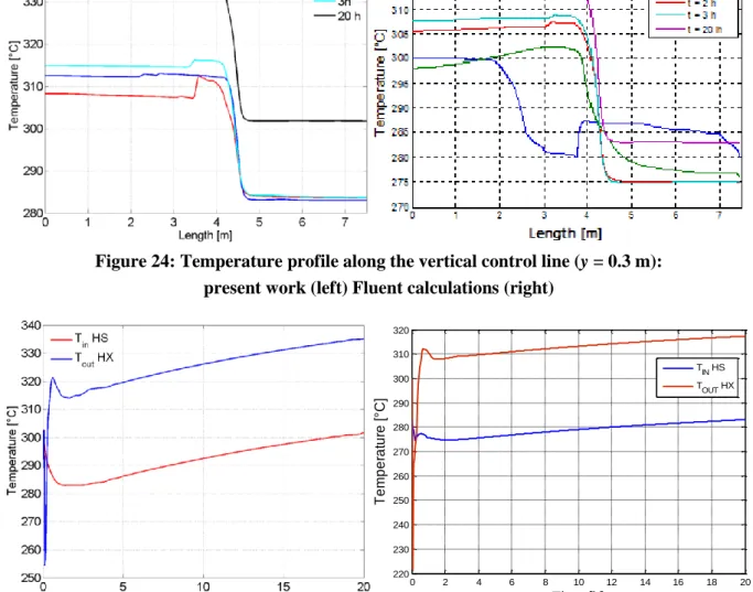
The temperature inside the LBE pool has been monitored along the vertical line at y = 0.3 m (already shown in Figure 17) and is compared with Fluent data in Figure 24. Results show, as expected, a similar qualitative trend. In particular, the temperature difference between lower and upper parts at 20h is approximately 34°C; the same value is obtained with Fluent. However, it can be noted that higher temperatures are present during the transient. In particular, at t = 20h the hottest temperature is about 335°C, while the hottest temperature obtained in Fluent is about 317°C.

Figure 24: Temperature profile along the vertical control line (y = 0.3 m): present work (left) Fluent calculations (right)

Figure 25: Temperature time trends at the outlet of the HX and at the inlet of the HS: present work (left) Fluent calculations (right)

This is confirmed by looking at Figure 25, which shows the trend over time of the LBE temperature at the inlet section of the HS and at the outlet section of the HX. During natural circulation flow regime, such trend is comparable and the same ΔT = 34°C is present; however, in the present work the temperatures increase faster over time. This difference is probably related to the coarse

0 2 4 6 8 10 12 14 16 18 20 220 230 240 250 260 270 280 290 300 310 320 Time [h] T e m p e ra tu re [ °C ] T_IN HS T_OUT HX

(23)

21

discretization of the domain and/or the selected model. In particular, numerical errors could be introduced that are amplified in the closed domain. Therefore, further work is recommended in order to investigate the effects of the discretization and selected model on the solution. However, it could be stated that, even with a coarse mesh, reasonably good information about the general trend of the flow are obtained and a good agreement is found between the two CFD codes. This confirms the capability of the solver to simulate heat transfer under thermally stratified conditions.

4. Development of a Coupled RELAP5-Fluent Model

In this part of the work, following the RELAP5-Fluent coupled models developed in the previous works for the NACIE loop type facility [1], [3], [4], a new modified and improved coupling tools has been performed for the CIRCE pool type facility. Due to the substantial difference between the two facilities layout (loop vs. pool type system), a new data exchange methodology for the coupled model between the boundaries of the STH domain and CFD domain has been adopted.

A first attempt of a coupled calculation with a CFD domain filled of LBE has been considered. The coupled system results however in an unstable model with non-physic results. Therefore, an open at the top of the CFD domain and the use of the VOF (Volume Of Fluid) model has been implemented.

Compared to the coupled tools described in [4] and to the previous works [1] [3], the computational efforts has been successfully enhanced developing a new methodology for interact with the Fluent code. The UDF (User Define Function) for the updating of the variables at the boundaries has been removed with no need to close and re-open the Fluent code at each time-step (and at each sub-iteration in the implicit version). The new methodology foreseen the launch of Fluent only at the beginning of the simulation by using the method “Fluent as a Server”. The new values of the variables exchanged between the codes are passed to Fluent in real time at each iteration by means of TUI (Text User Interface) tool using proper Matlab interface commands. With the use of this new technique the speed of the calculation has been improved by almost 4 times among the previous one.

4.1. Computational Domains and Mathematical Models

In this section, the computational domains and nodalizations adopted by the RELAP5 stand-alone and the RELAP5 and Fluent for the coupled model are presented. The pictures reported in this section constitute a very meaningful tool to clearly understand the logic of the coupled model. Moreover, the VOF mathematical model used for the Fluent domain is described.

4.1.1. RELAP5 Stand-Alone nodalization

The RELAP5 stand-alone nodalization of the CIRCE pool facility has been developed starting from a previous work [3]. The nodalization scheme adopted for CIRCE experiments simulations is depicted in Figure 26.

(24)

22

Figure 26: RELAP5 Stand – Alone nodalization of CIRCE facility

It is a pure 1-D system constituted by a total of 663 volumes and 678 junctions. The total mass of the LBE inside the facility is almost 70 tons at an initial constant temperature of 320°C. The pool of CIRCE is represented by the big pipe components numbered from 200 to 260. To simulate as better as possible the thermal stratification and phenomena as recirculation or horizontal flow path (especially during transient operation), a horizontal subdivision of the vessel has been performed. To avoid the connection of the volumes in cross-flow and to maintain a 1-D layout through all the system, some branch components have been interposed between the pipes (components 200, 210, 220, 230, 240 and 250). In the ICE section, the component pipe 60 simulates the FPS, component 90 represents the fitting volume and as described in the picture the component 130 is the riser. The Argon is injected by the time dependent junction 4 from the bottom of the riser (branch 100). The flow of the LBE mixed with the Argon rise then into the separator component (number 132). Then the LBE goes downwards through the Heat Exchanger 170 and enters in the pool, while the Argon

(25)

23

is separated. The yellow dotted area of component 170 represents the Heat Structures of the HX. The secondary system is represented on the right of the figure. On the left, the DHR system is connected to the hydrodynamic component of the pool 180 by means of the red dotted heat structure. The top part in white represents the cover gas above the LBE free surface.

4.1.2. Discretization of the coupled system

Since RELAP5/Mod.3.3 is a one dimensional system code, it is suitable for simulating the loop of the facility (ICE test section) including the FPS, Fitting Volume, Riser, Separator and the HX (both the primary and secondary side). The pool section constitutes the plenum of the reactor, in which ICE is immersed, and it is simulated by Fluent together with the DHR section. Due to the huge dimension of CIRCE facility main vessel and the long duration of the envisaged transient, a simplified 2D CFD geometrical domain was developed aiming at reducing the large computational power required. More specifically, the Fluent domain was modeled as a 2D axial-symmetric geometry, assuming the DHR's axis as axis of symmetry for the geometrical CFD domain. A better description of the two domains is given in the following section.

Figure 27 shows the CIRCE-ICE experimental facility subdivided into the two calculation domains. As already described, part A (ICE section) is simulated by RELAP5 while part B constitutes the Fluent computational domain.

The RELAP5 domain of the coupled simulation is represented in Figure 28.

(26)

24

Figure 28: RELAP5 part for coupled simulation – ICE + HX

The ICE nodalization has been already described in section 4.1.1. Figure 28 shows a more detailed picture of the nodalization in which the red numbers give the height of the volumes of the pipes. Compared to the stand-alone version the major changes are the addition of the two time dependent volumes 10 and 190, and the suppression of the big branch 150 (now is only a junction).

(27)

25

The CFD domain of the coupled simulation is represented in Figure 29 (the image is not in scale).

Figure 29: CFD domain – Pool + DHR

The cross section of the pool is divided in three different widths along the height of the facility: each cross section correspond to the real cross section at the corresponding height level. Starting from the top, the first width is obtained by subtracting the portion of area occupied by the HX and the Riser; the second width consider the space occupied by the Fitting Volume and the last cross

(28)

26

section is the total cross section of the pool minus the area of the FPS instrumentation. The level of the highest step on the right side of Figure 29 corresponds to the end of the HX and thus, it represents the inlet of the LBE in the pool domain. The outlet of the pool is obtained by drawing a little virtual "hole" in the centre of the domain (on the axis) placed at the same level of the FPS inlet and having the same area.

The DHR has been reproduced without simplifications and also the thickness of the walls has been modelled. In Figure 29 the inlet and the outlet of the air domain in the DHR are illustrated.

The simulation takes into consideration the Argon cover gas over the LBE in the pool (simulated with air) by using the VOF mathematical model of Fluent, described in Section 4.1.3 At the beginning of the simulation the cover gas is confined in the rectangle at the top of the domain (delimited by the dotted line) through the initialization of the volume fraction of the LBE. The top wall presents a small opening set as a pressure outlet condition to avoid the pressurization or depressurization of the pool, while on the rest of the wall a No Slip condition is applied. Note that the green mesh visible in Figure 29 is only represented to better understand the computational domain and it is different from the real mesh used.

The mesh has been created using the native tool of ANSYS Workbench. The final result is an almost complete structured mesh composed by quadrilateral elements with different aspect ratio. Only the region close to the end of the inner DHR tube is non-structured with quadrilateral dominant elements. Two different approaches based on the “first wall element distance” have been carried on during the mesh generation. First of all a coarse mesh with a total number of 242500 elements has been developed. This mesh has an average first element thickness such that the value of y+ is greater than 30; thus, in the standard k-ε turbulence model used, the "standard wall function" has been activated. Some details of the mesh developed are visible in Figure 30.

The second approach foresees the use of the "enhanced wall treatment" to resolve the boundary layer in the fluid regions (LBE and air) where high gradients of temperature and velocity are expected. These regions have been meshed with inflation layers on the walls such that the average distance of the first mesh element form the wall results in a value of y+ close to the unity. In particular, the refinement process has been confined to the fluid regions close to the DHR walls both for gas and LBE sides. For these purposes, the developed geometry was cut in 78 different surfaces to which special methods and different edges and faces sizing have been properly defined. To assure that the results of the simulations are not mesh depending, a proper grid independence study has been carried out. Three different meshes has been developed increasing each time the level of details (elements) especially around the DHR fluid domains to catch better the fluid-dynamic phenomena in the near-wall region. In order to compare the results of the steady state simulations among the different grids, the DHR has been activated by imposing a mass-flow air at the inlet boundary of 0.3 kg/s at room temperature (20 °C). Different variables have been monitored during the simulations to assure the achievement of a steady state solution.

The final grid accurately chosen and optimized for the enhanced wall treatment option has a total number of about 574500 elements. In order to have a value of y+ close to 1, the thickness of the first element in the LBE domain is about 50 µm and 20 µm for the Air domain. To maintain a reasonable total elements number, the mesh developed present an high aspect ratio (max A.R. = 200). Table 1

(29)

27

reports the parameters that express the statistics and qualities of the two compared meshes. Figure 31 shows some details of the finest mesh.

(30)

28

Figure 31: Fine mesh details (“Enhanced wall function”)

As already said all the meshes generated have been compared together simulating a constant mass flux of LBE at the inlet section of the pool and with the DHR active considering a constant air mass flow inlet of 0.3 kg/s. The results of the optimized coarse mesh (242500 elements and y+ > 30) have been then compared with the ones coming from the optimized fine mesh (574500 elements and

y+ ≈ 1). Figure 32 shows some details of the flow of the LBE and air inside the pool of the facility. Table 1: meshes parameters

COARSE MESH (y+ > 30) FINE MESH (y+ ≈ 1)

Elements number 242500 574500

Min. orthogonal quality 0.742 0.392

Max. skewness 0.570 0.779

(31)

29

(32)

30

From the previous results it is possible to note how the temperature distributions are not influenced by the different near wall treatments (“standard wall function” and “enhanced wall treatment”). Similar observation applies for the velocity profiles through all the computational domain. The resolution of the viscous layer close to the wall for what concern temperature and velocity is obviously higher in the finer mesh, but, since we are more interested in reproducing the general flow path and temperature distribution of the LBE in the pool, the coarse mesh has been considered as the best compromise between accuracy and time effort. Moreover, a coupled simulation requires large computational time and resources and a high quality mesh with low number of elements is fundamental.

4.1.3. VOF model

The VOF model [12] is used in Fluent to permit the correct simulation of the cover gas above the LBE free surface in the pool.

The VOF formulation relies on the fact that two or more fluids (or phases) are not interpenetrating. For each fluid added to the model, a variable is introduced: the volume fraction of the fluid in the computational domain cells. In each control volume, the volume fractions of all phases sum to unity and the fields for all variables and properties are shared and represent volume-averaged values. Thus the variables and properties in any given cell are either purely representative of one of the phases, or representative of a mixture of the phases, depending upon the volumefraction values. If the qth fluid's volume fraction in the cell is denoted as αq, then the following three conditions are possible:

• αq = 0 : the cell is empty (of the qth fluid). • αq = 1 : the cell is full (of the qth fluid)

• 1 < αq < 0 : the cell contains the interface between the qth fluid and one or more other fluids.

In the upper part of the pool, the free surface between the Argon gas and the LBE is simulated and the position of the gas-liquid interface is tracked during the transient. Moreover, being the fluids immiscible, the free surface will results a clearly defined interface for which the cells contains a mixture of two fluids (LBE and Argon). In the post-processing the free surface is individuated by an iso-surface line for which the value of LBE (or Argon) volume fraction is equal to 0.5. In this way it is possible to track the level of the LBE in the pool of the facility.

(33)

31

Figure 33: LBE Volume fraction initialization for the VOF model

4.2. Coupling procedure and strategies

The logic scheme of the coupled model created is represented in Figure 34. The main difference with the previous coupled code created by Martelli et al. [4], is constituted by the thermodynamic variables exchanged at the interfaces between the domains. A first simulation in which, at the inlet of ICE (bottom of the pool) RELAP5 give the pressure to Fluent and receive from it the values of mass flow and temperature, while, at the outlet of ICE Fluent give the pressure to RELAP5 and receive from it the values of mass flow and temperature has been found unstable when applied to the simulation of the CIRCE pool type facility. Indeed, a small variation of the pressure given by RELAP5 at the outlet of the pool results in very large variation of the LBE mass flow rate entering the pool mainly due to the large dimension of the pool. Therefore, a new coupling methodology has been developed. As can be note from Figure 34, Fluent gives to RELAP5 the pressures both at the inlet and outlet section of ICE, while at the same time RELAP5 gives the mass flows (velocities) at the inlet and outlet of the pool (CFD domain). The temperature are given to the Fluent pool inlet by RELAP5 (temperature of the volume at the exit of the HX) and vice versa, at the interface in the bottom Fluent gives the temperature to the time-dependent volume 10 of RELAP5.

(34)

32

(35)

33

This strategy yields a stable behaviour to the simulation of a pool type facility like CIRCE. For that reason the inlet and outlet sections of the CFD domain has been set respectively as a velocity-inlet and velocity-outlet boundaries. The velocities have been set normal to the surfaces. The outlet of the Heat Exchangers consist in a sudden big enlargement and the pressure drops are calculated automatically by Fluent; the inlet of the FPS section constitutes instead a sudden restriction and to take into account the pressure drops, a proper K loss factor of 0.5 has been imposed at the inlet junction number 15 of RELAP5.

4.2.1. Implicit coupling scheme

The numerical method adopted for the coupled simulation is the implicit scheme shown in Figure 35. In a numerical implicit method, the solution is found by solving an equation involving both the current state of the system and the later one. As shown, each time step has to be repeated several times updating boundary conditions (b.c.) at each “inner-cycle” (red dotted line) until specified convergence criteria are satisfied; after that both codes proceed to compute b.c. for the next time step. Each time step, both for outer and inner iterations, foresees the exchange of the variables (pressures, temperatures and velocities) between the boundaries of the two codes according to the scheme reported in Figure 34.

It is clear that implicit methods require a higher computational cost and they can raise greatest difficulties in terms of implementation with respect to the explicit coupling scheme. On the other hand, they own valuable advantages: strong numerical stability and the possibility to use relatively larger time step compared to the explicit coupling method (especially for stiff problems).

Each inner iteration can be repeated until specified convergence criteria is satisfied or, for a simplified programming, setting a fixed number of inner iterations for each time step. For the performed simulations, a fixed number of inner iteration was imposed and from a first sensitivity analysis, three inner iterations per each time step was chosen as a good compromise between CPU time and accuracy of results.

First, a RELAP5 calculation with boundary conditions coming from the first initialization of Fluent was started to find the initial steady state condition at a fixed temperature of 280°C and with fluid at rest. The end of this first RELAP5 transient calculation (1000 seconds) has been considered time zero from which the coupled simulation starts.

The Fluent code (master code) advances firstly by one time step and then the RELAP5 code (slave code) advances for the same time step period, using data received from the master Fluent code. At the beginning of each inner cycle iteration of Fluent a linear interpolation of the three RELAP5 boundary condition data between the initial and the final value of the calculated time step is performed (see Figure 35).

(36)

34

Figure 35: Implicit coupling scheme

4.2.2. Improvements of the new coupled code

A new logic to manage the Fluent code from Matlab has been developed. Previous versions of the coupled codes developed for NACIE facility foresee the use of a parallelized User Define Function (UDF) to read at the beginning of the iteration the thermodynamic variables coming from RELAP5, to specify the new boundary conditions and to write at the end of the iteration the three variables in different “.txt” files. A Journal file was used to load at each iteration the Fluent “case” and “data”, to run the solver and to close the Fluent again. The opening of the Fluent and the action of reading the “case” file and the UDF, are high time consuming compared to the time requested for the calculation of each iteration.

(37)

35

The basic idea of the new implemented logic is to open Fluent from Matlab only at the beginning of the simulation in Server mode (“Fluent as a Server”) on the Local PC used. The use of an add-ons of Fluent, called CORBA, allows the creation of an interface between Matlab and Fluent as a Server so that it is possible to manage the Fluent session through TUI specific commands. In this way, the use of the UDF and Journal file are no more necessary and the opportunity of leaving Fluent open with the case always loaded takes great advantage in terms of the global computational time. This improvements speed up the calculation reducing the computational costs by roughly four times compared to the previous technique.

Figure 36 shows the logic of the coupled code in a schematic way.

Figure 36: New coupled code scheme

4.3. Simulation Tests

The developed implicit coupling scheme was adopted to simulate an experimental test representative of a gas enhanced circulation test and reported in Table 2.

The argon is injected in the RELAP5 model through the time dependent junction 4 (see Figure 34). Its value, is set as boundary condition in agreement with the mass flow rate fixed in the experiment (averaged over each steps) as shown in Figure 37.

(38)

36

Table 2: Forced circulation test

T[°C] FPS Power % HX Power % Gas_lift [Nl/s]

280 0 0 Step 1 1.9 Step 7 4.5 Step 2 2.3 Step 8 4.9 Step 3 2.7 Step 9 4.1 Step 4 3.1 Step 10 3.1 Step 5 3.7 Step 11 2.2 Step 6 4.1 - -

Figure 37: Argon mass flow rate – Input data for simulations

The red line represents the averaged experimental data assumed as input condition in the simulations. Two different simulations have been performed and are described in Table 3.

Table 3: Matrix of performed simulations

Name Time Step CFD Geometrical Domain Serial/Parallel RELAP5 Stand – alone Max Courant limit - serial

Fluent + RELAP5

(39)

37

As mentioned in Section 4.2.1, the implicit scheme allows larger time steps and is more stable than the explicit scheme. Anyway, in order to achieve an appropriate accuracy, the time step shall be chosen reasonably small. For this reason, a sensitivity analysis of the time step is carried out providing as a result that the implicit coupling scheme allows the use of a time step of 0.025 s without losing in results accuracy.

4.4. Obtained results

In Figure 38 the obtained RELAP5 stand-alone results are compared to the experimental data. Good agreement is found with a trend that generally tend to underestimate the experimental LBE mass flow rate for the lower Argon mass flow rate and vice versa for the higher steps. The maximum error committed in the estimation of the LBE mass flow rate is lower than 3.3%.

Figure 38: LBE mass flow rate time trend

For the Fluent RELAP5 coupled simulation, eleven different simulations corresponding to the eleven steps of Argon mass flow rate were performed. Each simulation starts from a condition in which the fluid is at rest both in RELAP5 and Fluent domains. The results obtained from the coupled simulation of Step 2 are reported from Figure 39 to Figure 41. In particular, in Figure 39 the LBE mass flows at the interface between the two domains (inlet and outlet of RELAP5 nodalization) are compared with the experimental data. As it can be seen, the results coming from the coupled simulations agree well with the experimental data as soon as steady state conditions are reached (see Figure 39). Figure 40 reports respectively the evolution of the pressures at the inlet and outlet boundaries of the CFD domain (corresponding to the outlet and inlet of RELAP5 domain). In Figure 41, the height of the LBE in the separator component (pipe 135 of Figure 34) and in the pool are shown. The squared trend of the pool level is due to the mesh resolution and to the

(40)

post-38

processing method. As can be seen from the comparison of the two charts, at the beginning of the simulation the LBE level in the pool and in the separator correspond (the fluid in the facility is at rest) while after the Argon gas injection different heights due to the pressure drops in the ICE loop are evidenced. Differences in height of the LBE between pool and separator increase with Argon injection, and for the values of mass flow rate of Argon injected considered in the simulations, they range from a minimal value of 12 mm to a maximum of 27 mm.

Figure 39: ICE Inlet and Outlet LBE mass flow rate for coupled simulations Step 2

(41)

39

Figure 41: Separator and pool LBE height level

Figure 42 and Figure 43 show respectively the calculated LBE mass flow values obtained for other two coupled simulation: Step 4 and Step 6. Also in these cases, it is possible to observe how the calculated LBE mass flow rates agree well with the experimental data.

(42)

40

Figure 43: LBE mass flow rate for coupled simulation Step 6

Finally, in order to resume all the performed simulations (RELAP5 Stand-alone and the 11 coupled Fluent-RELAP5 simulations), the calculated LBE mass flow rate is plotted as a function of the experimental mass flow rate for all the eleven steps (averaging the experimental data over the steps, see Figure 44). Calculated results satisfactory predict the experimental data (most of the obtained results lies in a range between +5% and -5%) with a trend that generally tend to underestimate the experimental LBE mass flow rate at lower values of Argon flow rate injected and to overestimate it at the highest ones. A better tuning of RELAP5 pressure drops into the ICE section should led to enhance the agreement between calculated and experimental results.

(43)

41

Figure 44: Experimental vs calculated LBE mass flow rate for RELAP5 stand – alone and coupled simulations

5. Conclusions

The present work consist of two main parts, aimed at contributing to the development and improvement of a coupling methodology between CFD codes and thermal-hydraulic system codes for pool-type facilities like CIRCE. In the first part of the work, CFD simulations of a PLOHS+LOF accidental scenario inside CIRCE facility were carried out using the STAR-CCM+ code. For this purpose, two URANS simulations were performed with different boundary conditions using a 2D computational domain. In the first simulation, the boundary conditions applied in the CFD code were extracted from CIRCE Test I experimental data; whereas in the second one the imposed boundary conditions were taken from a previous RELAP5 calculation, using a “one-way” coupling methodology between the two codes. Preliminary calculations were performed with a coarse discretization in order to verify the correct implementation of such boundary conditions into STAR-CCM+ and to obtain an initial qualification of the capability of the CFD solver to reproduce a thermally stratified flow. The comparison between the obtained results and experimental data showed the same time trend of the main variables; however, some discrepancies are present because heat losses towards the external environment and the internal structures were not implemented. However, results showed good agreement compared to a previous “one-way” Fluent/RELAP5 coupled calculation. This confirms a good capability of STAR-CCM+ to reproduce heat transfer under thermally stratified conditions. In order to improve the model, further work is needed by studying the influence of the discretization and the numerical method on the results. Moreover, to obtain a high quality solution, heat transfer towards the environment has to be considered.

(44)

42

In the second part of this work, a “two-way” implicit coupling method was developed between Fluent and RELAP5 codes for a gas enhanced circulation test inside CIRCE facility. In this case, a 2D CFD domain is adopted to reproduce the pool of the facility, whereas the ICE test section is modelled with the RELAP5 STH. In order to simulate the cover gas in the pool of the facility, the VOF (Volume Of Fluid) model of Fluent was implemented. A mesh sensitivity analysis was performed in order to find the best compromise between the required computational power and quality of the results. Moreover, the computational efforts were successfully enhanced by the use of a new methodology for interact with the Fluent code using MATLAB. Obtained results of the coupled simulation were compared to the experimental data together with the ones coming from a RELAP5 stand-alone calculation (also performed in this work). Such comparison highlights the good agreement among each other with a maximum error of 3.3%. Moreover, the new coupling methodology improves the velocity of calculations reducing it by a factor 4-5 compared to the previous works.

In order to confirm the capability of the coupled Fluent/RELAP5 model to simulate CIRCE facility at nominal conditions (forced convection together with activated FPS and HX) and PLOHS+LOF accidental scenario, further improvements needs to be done.

Finally, verification and validation of coupled methodologies with CFD codes using a 3D computational domain have to be performed in order to obtain a more realistic three-dimensional solution.

(45)

43