396 социальНо-экоНомические проблемы региоНа
For citation: Ekonomika regiona [Economy of Region]. — 2016. — Vol. 12, Issue 2. — pp. 396-404 doi 10.17059/2016–2–6
UDC 364.22
JEL Classification: C21, I32, C23
F. Crescenzi, G. Betti, F. Gagliardi University of Siena (Siena, Italy; e-mail: [email protected])
Comparing Small area TeChniqueS
for eSTimaTing poverTy meaSureS:
The CaSe STudy of auSTria and Spain
1The Europe 2020 Strategy has formulated key policy objectives or so-called “headline targets” which the European Union as a whole and Member States are individually committed to achieving by 2020. One of the five headline targets is directly related to the key quality aspects of life, namely social inclusion; within these targets, the European Union Statistics on Income and Living Condition (EU-SILC) headline indicators at-risk-of-poverty or social exclusion and its components will be included in the budgeting of structural funds, one of the main instruments through which policy targets are attained. For this purpose, Directorate-General Regional Policy of the European Commission is aiming to use sub-national/regional level data (NUTS 2). Starting from this, the focus of the present paper is on the “regional dimension” of well-being. We propose to adopt a methodology based on the Empirical Best Linear Unbiased Predictor (EBLUP) with an extension to the spatial dimension (SEBLUP); moreover, we compare this small area technique with the cumulation method. The application is conducted on the basis of EU-SILC data from Austria and Spain. Results report that, in general, estimates computed with the cumulation method show standard errors which are smaller than those computed with EBLUP or SEBLUP. The gain of pooling SILC data over three years is, therefore, rel-evant, and may allow researchers to prefer this method.
Keywords: small area estimation, poverty, EU “headline targets”, regional level, NUTS-2, inequality, SEBLUP, cu-mulation, SILC, Austria, Spain
1
1. Introduction
In the last two decades, there has been the in-creased interest in the comparative analysis of poverty and social exclusion in the European Union. The Statistical Office of the European Union (Eurostat) launched the European Community Household Panel study (ECHP, 1994– 2001) and later the EU Statistics on Income and Living Conditions (EU-SILC, 2004-to date), in or-der to create a European standardised data base to generate comparative measures of poverty and so-cial exclusion among the Member States. A com-prehensive set of common indicators, termed the Laeken Indicators, has been adopted for countries of the European Union [1]. These indicators are produced on a regular basis at the national level, and are mainly based on the EU-SILC. EU-SILC surveys involve a rotational panel design con-ducted annually in each country. Microdata from the surveys are available to the research commu-nity in the form of Users’ Data Base (UDB). The na-tional sample designs and sizes have been deter-mined primarily for the purpose of estimation and reporting of indicators at the national level, with 1 © Crescenzi F., Betti G., Gagliardi F. Text. 2016.
a limited breakdown by major socio-demographic subgroups of the population.
The Europe 2020 Strategy 2 has formulated key policy objectives or so-called “headline targets” which the EU as a whole and Member States indi-vidually are committed to achieving by 2020. One of the five headline targets is directly related to the key quality aspects of life, namely social inclu-sion; within these targets, the EU-SILC headline indicators at-risk-of-poverty or social exclusion (AROPE, which is also known as Head Count Ratio (HCR) and FGT(0) in the family of [2]) and its com-ponents will be included in the budgeting of struc-tural funds, one of the main instruments through which policy targets are attained.
For this purpose, DG Regional Policy of the European Commission is aiming to use sub-na-tional/ regional level data (NUTS 2 3, and excep-tionally NUTS 1 for a couple of big countries) for the social headline indicators, in order to com-plement GDP per capita, in defining regions that 2 European Commission, Communication from the Com- mission. Europe 2020. A strategy for smart, sustainable and in-clusive growth. Brussels, 3.3.2010 COM(2010) 2020, 2010. 3 NUTS is an abbreviation for Nomenclature of Statistical Territorial Units. This is Eurostat’s hierarchical classification of regions, from Member States (NUTS 0) down to smaller areas.
can apply for funding directed to the Convergence Objective. As a first step in this direction, for the funding period 2014–2020, these indicators will be used for benchmarking and assessing the ef-ficiency of regional policies and programmes. Therefore, there is an urgent policy need for re-gional values of social policy indicators. The fo-cus should be on accurately and correctly identify-ing regions with the highest proportion of people being poor or socially excluded, in order to target policy measures accordingly. For these reasons, the focus of the present paper is on the “regional dimension” of well-being. While the above-men-tioned EU-wide comparative data sets, namely the ECHP and the EU-SILC, can serve as unique sources for generating comparative indicators of well-being, or rather of lack of welfare manifest such as poverty and deprivation, these sources are designed primarily to serve at national level, and appropriate methodologies are required to extend their use to the level of sub-national regions: such methodologies are known as small area estima-tion (SAE) techniques.
There is a wide variety of techniques available (SAE) in the literature, and the field is rapidly ex-panding. The suitability and efficiency of a par-ticular technique depend on the specific situation and the nature of the statistical data available for the purpose. The standard reference on small area estimation methodology are [3], [4] and, above all, [5]; [6] focus on small area estimation methods for poverty and inequality measures.
One class of techniques aims at making the best use of available data from national sample surveys, such as by cumulating and consolidating the information to obtain more robust measures which permit greater spatial disaggregation; this class is described in Section 2, where the particu-lar method of cumulating three-years of the EU-SILC survey is described and applied.
Another class of techniques is based on small area models; in the literature these are classified as: (i) area level random effect models [7], which are used when auxiliary information is available only at area level (such as the prevailing unem-ployment rate); (ii) nested error unit level regres-sion model, used if unit specific covariates (such as the individual’s or the household’s employment situation) are available at unit level [8].
In Section 3, one technique of class (i) is taken into account, namely the Empirical Best Linear Unbiased Predictor (EBLUP), and its develop-ments in a spatial environment. One well-known methodology of class (ii) is often undertaken by the World Bank, namely the Poverty Mapping ([9], ELL); however, it requires direct access to census
data, which is not usually available for university researchers.
Finally, in Section 4 we compare the results ob-tained by the cumulation method and the spatial EBLUP (SEBLUP) method, based on Austria and Spain; some concluding remarks are also reported at the end of the paper.
Both methodologies applied in Sections 2 and 3 are based on the SILC, which is the major source of comparative statistics on income and living con-ditions in Europe. EU-SILC covers data and data sources of various types: cross-sectional and lon-gitudinal; household-level and person-level; on income and social conditions; and from registers and interview surveys depending on the country. A standard integrated design has been adopted by nearly all EU countries. It involves a rotational panel in which a new sample of households and persons is introduced each year to replace one quarter of the existing sample. Persons enumer-ated in each new sample are followed-up in the survey for four years. The design yields each year a cross-sectional sample, as well as longitudinal samples of various durations.
2. Cumulative measures of poverty This section focuses on pooling of differ-ent sources pertaining to the same population or largely overlapping and similar populations. In particular, the interest is in pooling over survey waves in a national survey in order to increase the precision of regional estimates. Estimates from samples from the same population are most effi-ciently pooled with weights in proportion to their variances (meaning, with similar designs, in direct proportion to their sample sizes). Alternatively, the samples may be pooled at the micro level, with unit weights inversely proportional to their prob-abilities of appearing in any of the samples. This latter procedure may be more efficient (e.g.,[10]), but may be impossible to apply as it requires in-formation, for every unit in the pooled sample, on its probability of selection into each of the sam-ples irrespective of whether or not the unit actu-ally appears in the particular sample [11]. Another serious difficulty in pooling samples is that, in the presence of complex sampling designs, the struc-ture of the resulting pooled sample can become too complex or even unknown to permit proper variance estimation. In any case, different waves of a survey like EU-SILC do not correspond to ex-actly the same population. The problem is akin to that of combining samples selected from multi-ple frames, for which it has been noted that micro level pooling is generally not the most efficient method [12]. For the above reasons, the
pool-398 социальНо-экоНомические проблемы региоНа
ing of wave-specific estimates rather than of mi-cro data sets is generally the more appropriate ap-proach to aggregation over time from surveys such as EU-SILC.
2.1. Gain in precision from cumulation over survey waves
Consider that for each wave of a survey like EU-SILC, a person’s poverty status (poor or non-poor) is determined from his/her income within the in-come distribution of that wave, independently for each EU-SILC year, and then the proportion of poor at each wave is computed. These proportions are then averaged over a number of consecutive waves. The issue is to quantify the gain in sam-pling precision from such pooling, compared to results based on a single wave.
The quantification of efficiency gains from av-eraging across multiple years is not straightfor-ward in surveys, such as EU-SILC, that are based on rotational panel, given that data from different waves of a rotational panel are highly correlated.
A large proportion of the individuals is com-mon in the different cross-sections. However, a certain proportion of individuals is different from one wave to the other. The cross-sectional sam-ples are thus not independent, resulting in a cor-relation between measures from different waves.
Apart from correlations at the individual level, we have to deal also with an additional corre-lation that arises because of the common struc-ture (stratification and clustering) of the waves of a panel. Such correlation would exist in, for in-stance, samples coming from the same clusters even if there is no overlap in terms of individual households.
In order to quantify the gain in precision from averaging over waves of a rotational panel, we pro-vide the following simplified procedure that could be of help in better clarifying the point. It illus-trates the statistical mechanism of how the gain is achieved.
Indicating by pj and p′j the (1, 0) indicators of poverty of individual j over the two adjacent waves, we have the following result for the popu-lation variances:
(
)
2 var( )pj =∑
p pj- =p(1-p)=V; similarly, var( )p′j =p′(1-p′)=V′, ' 1 cov( , )p pj ′j =∑
(p p pj- )( jj′-p′)= - ⋅ =a p p c′ ,where ‘a’ is the persistent poverty rate over the two adjacent years. Under the two waves model and in the extreme case of a completely full sample over-lap and p′ = p, the variance VA of the average over two waves of the concerned poverty measure can be estimated as: (1 ), 2 A V V = + ρ (1) where ρ represents the correlation between the two waves that in our simplified case can be
quan-tified by 1 2 2 . c a p V p p -ρ = = - -
Alternatively, if the overlap between the two waves is only partial like in the EU-SILC sur-vey, and cross-sectional variances are not nec-essarily equal, it is necessary to allow for vari-ations in cross-sectional sample sizes and par-tial overlaps: 1 2 1 1 , 2 2 A H V V n V n + = + ρ (2)
where V1 and V2 are the variances in each of the two waves, n is the sample overlap, nH is the har-monic mean of different wave sizes, ρ as above [13].
2.2. Quantifying the gain in sampling preci-sion using EU-SILC survey
The formula presented in Section 2.1 have been applied to the EU-SILC cross-sectional datasets in order to obtain averaged measures over waves.
When complete information on sample struc-ture is available and, more specifically, when identifiers are provided to link strata and PSUs throughout different EU-SILC cross-sectional da-tasets, it is possible to cumulate waves and quan-tify the gain in sampling precision achieved with this methodology. When the above requirement is met, that is when full information on sample structure is available, the gain in sampling pre-cision can be easily quantified by applying the standard JRR methodology presented above on the basis of the following considerations.
The total sample of interest is formed by the union of all the cross-sectional samples being compared or aggregated. Using the common struc-ture of this total sample as a basis, a set of JRR rep-lications is defined in the usual way.
Each replication is formed in such a way that when a unit is to be excluded in its construction, it is excluded simultaneously from every wave where the unit appears.
For each replication, the required measure is constructed for each of the cross-sectional sam-ples involved, and these measures are used to ob-tain the required averaged measure for the repli-cation. The variance of the statistic of interest is then estimated from the replication estimates in the usual way.
Let us clarify this procedure, presenting an empirical example. Consider that we have the cross-sectional dataset of the EU-SILC survey for
three consecutive years and want to estimate the average of a given poverty measure over the three years. We proceed as follows. We first construct a common structure of strata and PSUs from the union of the three cross-sectional datasets; that is, we keep the list of all the strata and PSUs of each of the three datasets and construct a new list that is the result of the union of the three sam-ples. Then we will create the replications from this common structure.
In the standard JRR methodology, replications are created by eliminating one PSU at a time, a replication being identified by the particular PSU (say k) eliminated in constructing it. In the com-bined dataset, the concerned PSU, if present, is eliminated from all the three cross-sectional da-tasets to obtain a ‘combined’ replication.
For each year (t) and for each replication (k), we can estimate ( )t
k
y and from this, the required statis-tic, as follows: (1) (2) (3) ( ) / 3. Average k k k k y = y +y +y (3) The variance estimate of this measure can be estimated applying the JRR procedure for variance estimation proposed by [14], using the ‘combined’ replications as defined above, as if the statistic were a common cross-sectional measure.
It is necessary to underline again that such procedures can be applied only if full information on the sample structure is available.
We have developed an alternative procedure for dealing with a situation in which full informa-tion on the sample structure is lacking [15].
2.3. Empirical results
We have applied the methodologies described above to calculate the average measures for three years (2009, 2010 and 2011) to EU-SILC data for Austria (AT) and Spain (ES). The empirical anal-ysis has been performed only on these two coun-tries for the following reasons. In the public ver-sion of the EU-SILC data, the so-called UDB, the variables necessary for constructing the structure of the sample (namely, the PSUs ‘DB060’ and the strata ‘DB050’) are not present and no link is pos-sible across cross-sectional dataset either at mi-cro (unit) level or at mami-cro (structure) level. This problem is reflected also in Section 3. Thanks to a project with the OECD for Spain we had access to all the necessary information on the sample struc-ture and the linkage of the cross-sectional data-sets. For Austria, all necessary information (link-age of the structure for the 3 cross-sectional data sets) was not available to us, but, given that the Austria sample structure could be assimilated to a simple random sampling, we used for the com-putation the indirect procedure, mentioned above.
Results at the national level for Austria and Spain are shown in Table 1, and results at regional NUTS 2 level in Austria and Spain in Table 2 and 3.
The results at the national level show a sensi-ble reduction of the standard error (s.e.) using the three years average with the two measures con-cerned. The reduction of the standard errors that we get using the three years averages compared to the estimate for a single year (column (d)), ranges from 12 % for S80/S20 index for Austria, up to 35 % for HCR for Spain. In general, the two methodolo-gies (direct and indirect) for the estimation of the standard errors of averaged measures over three years perform well and give similar results both at
Table 1
Average over three years, Austria and Spain
(a) (b) (c) (d) AUSTRIA HCR 60 % national p.l. 13.8 0.608 0.426 0.700 S80/S20 4.0 0.084 0.066 0.786 SPAIN HCR 60 % national p.l. 22.0 0.478 0.311 0.650 S80/S20 6.5 0.154 0.110 0.718
(a) estimate 2011; (b) s.e. 2011; (c) s.e. 3-years average; (d) ratio s.e. 3-years average over s.e. single year.
Table 2
Average over three years, Austria regional NUTS 2 level HCR 60 %, national p. l. (a) (b) (c) Burgenland 3.721 2.438 0.655 Niederösterrich 1.065 0.783 0.735 Wien 1.859 1.352 0.727 Kärnten 3.347 2.240 0.669 Steiermark 1.297 1.100 0.848 Oberösterrich 1.119 0.718 0.642 Salzburg 1.877 1.323 0.705 Tirol 1.914 1.146 0.599 Voralberg 1.989 1.595 0.802 Mean 0.709 Median 0.705 S80/S20 Burgenland 0.477 0.323 0.677 Niederösterrich 0.177 0.138 0.780 Wien 0.225 0.169 0.751 Kärnten 0.315 0.238 0.754 Steiermark 0.218 0.163 0.749 Oberösterrich 0.181 0.140 0.773 Salzburg 0.361 0.257 0.712 Tirol 0.303 0.217 0.715 Voralberg 0.425 0.405 0.951 Mean 0.763 Median 0.751
(a) s.e. 2011; (b) s.e. 3-years average; (c) ratio s.e. 3-years aver-age over s.e. single year.
400 социальНо-экоНомические проблемы региоНа
the national and regional level, as we have already shown in our past work. The comparison of stand-ard errors between one-year and three-year esti-mates is more complex at regional NUTS 2 level, given the instability of the one-year estimates be-cause of small samples. This problem is particu-larly evident for regions with a small number of PSUs. The cumulated estimates, in fact, have been chosen to overcome to the high instability of the single year estimates.
Generally, also in this case, we can appreciate a reduction of the standard error, both in mean and median, for the two measures. The reduction can be better appreciated considering the median, which is not affected by extreme values that are present in the results given the instability of the estimates for single years.
The results are very stable across regions in Austria. Furthermore, the results for mean and median measures are nearly the same, showing a reduction in variance of about 25–30 % with pool-ing over 3 years.
For Spain, the largest reductions, in this case, are in S80/S20, where, in median, we have a de-crease of 38 %; for HCR the dede-crease in median is 20 %.
3. Model-based small area estimation In this section, we present the main features of some model-based techniques for small area esti-mation, namely, the EBLUP estimator based on the model by [7] and the EBLUP estimator based on spatially correlated random effects [16]. The first is an essential tool in dealing with small area esti-mation when only aggregated auxiliary data at the area level are available, the latter allows for spatial dependence of area-level random effects by as-suming a Simultaneously Autoregressive Process (SAR). We have applied these estimators to a pair of poverty and inequality measures, namely Head Count Ratio and the S80/S20 index.
3.1. Empirical Best Linear Unbiased Predictor We are interested in obtaining an estimate of a domain specific parameter. In this work, it can be either HCR or S80/S20. As true values are un-known, it is assumed that a design-based unbiased estimator of the parameter is available such that:
ˆ ,
i i ei
θ = θ + (4)
where ei, are the sampling errors for each area. It is known as sampling model. It is assumed that the sampling variances are known, but in practice, it is rarely the case, so they are replaced with esti-mates obtained by following a JRR procedure [17]. It is further assumed that true values are linearly related to a vector of area specific auxiliary
varia-Table 3a
Average over three years, Spain regional NUTS 2 level, HCR HCR 60 %, national p. l. (a) (b) (c) Galicia 1.167 0.828 0.710 Principado de Asturias 1.035 0.708 0.684 Cantabria 0.948 2.084 2.199 País Vasco 0.840 0.475 0.565
Comunidad Foral de Navarra 0.831 0.602 0.725
La Rioja 1.502 0.980 0.653 Aragón 1.521 2.720 1.788 Comunidad de Madrid 1.908 0.931 0.488 Castilla y León 1.388 1.327 0.956 Castilla-La Mancha 1.735 1.183 0.682 Extremadura 2.045 2.326 1.137 Cataluña 1.033 0.549 0.531 Comunidad Valenciana 1.007 1.040 1.033 Illes Balears 1.127 1.845 1.637 Andalucía 1.175 0.944 0.804 Regíon de Murcia 1.563 1.313 0.840
Ciudad Autónoma de Ceuta 1.340 2.460 1.837
Ciudad Autónoma de Melilla 2.154 1.514 0.703
Canarias 1.187 1.071 0.902
Mean 0.993
Median 0.804
Table 3b
Average over three years, Spain regional NUTS 2 level, S80/S20 S80/S20 Galicia 0.359 0.180 0.503 Principado de Asturias 0.423 0.221 0.521 Cantabria 0.286 0.222 0.777 País Vasco 0.284 0.167 0.587
Comunidad Foral de Navarra 0.479 0.193 0.402
La Rioja 0.539 0.276 0.511 Aragón 0.358 0.247 0.690 Comunidad de Madrid 0.249 0.206 0.827 Castilla y León 1.644 0.597 0.363 Castilla-La Mancha 0.968 0.466 0.482 Extremadura 0.586 0.363 0.619 Cataluña 0.286 0.165 0.579 Comunidad Valenciana 0.414 0.271 0.655 Illes Balears 0.476 0.427 0.897 Andalucía 0.515 0.313 0.607 Regíon de Murcia 0.354 0.384 1.084
Ciudad Autónoma de Ceuta 0.392 0.846 2.156
Ciudad Autónoma de Melilla 0.933 0.639 0.684
Canarias 0.523 0.840 1.606
Mean 0.766
Median 0.619
(a) s.e. 2011; (b) s.e. 3-years average; (c) ratio s.e. 3-years average over s.e. single year
bles. Normality of random effects can be assumed to obtain Maximum Likelihood (ML) or Restricted Maximum Likelihood (REML) estimates. This model is known as linking model. By combining the above results we can get the following model proposed by [7]:
ˆi i′ z v ei i i.
θ =xβ+ + (5) The Best Linear Unbiased Predictor can be eas-ily obtained by applying the general results of lin-ear mixed effects models and it is equal to:
( )
2 ˆ(
1)
, H i v i i i i′ θ σ = g θ + - g x β (6) where factor 2 2 ( 2 2) i zi v i zi v g = σ ψ + σ is known asshrinkage factor. The expression above shows that the BLUP estimator is an average of the direct es-timator and of the synthetic eses-timator. It can be noted that the lower the sampling variance is, the more the weight is attached to the direct estima-tor, in fact, when ψi → 0 then gi → 1 meaning that
ˆ .
H
i i
θ → θ We can say that the BLUP estimator is
de-sign consistent.
The BLUP estimator is unknown as it depends on random effects variance. By substituting it with a consistent estimator, we obtain a two stage esti-mator which can be referred to as Empirical BLUP (EBLUP).
The classic Fay and Herriot model (5) can be extended by considering that the vector of errors vi follows a Simultaneously Autoregressive Process (SAR) with spatial autoregressive coefficient ρ and proximity matrix W [18].
In this way, the model with spatially correlated random effects is the following:
(
)
1ˆ X Z I W - u e.
θ = β + - ρ + (7)
Matrix W describes the spatial contiguity among areas while ρ describes the strength of spa-tial relationship among the random effects associ-ated with neighbouring areas.
Under the model (7) it is straightforward to de-velop the Spatial Best Linear Unbiased Predictor, which is equal to the classic BLUP if the autocorre-lation coefficient is equal to zero. The estimator is unknown because it depends on unknown param-eters. By substituting them with consistent esti-mators (ML or REML), the model results to be as a Spatial EBLUP [16].
The spatial weight matrix reflects the neigh-bouring structure of the small areas. In the next applications, the structure has been specified by following an approach based on contiguity and on distance threshold (see [19] for further details).
The former specifies the spatial dependence between two areas by assigning spatial weight wij = 1 if area i and j are adjacent and zero
other-wise. Generally, the matrix W is row-standardized, so it is row-stochastic and ρ is called a spatial au-tocorrelation parameter [20].
3.2. Applications
In this section, we apply the above estimators to EU-SILC data available for Austria and Spain at NUTS2 level for the year 2011 and for two poverty measures, the HCR and S80/S20.They are the same data used in Section 2.3. Following [21] there are basically three different types of spatial data: 1) Spatial Point Processes 2) Geostatistical data 3) Areal Data. In this paper, we focus on areal data which means that when it is collected data regard a particular region, country, small area of any kind. The aim is to investigate how and to what extent data observed in one region is influenced by what has been observed in other regions. We present EBLUP and SEBLUP estimates for both countries, Spain and Austria.
For the HCR in Spain, the Spatial EBLUP based on a distance approach leads to the highest gain in efficiency (about 3 %) 1. The gain is quite small, this is due to the fact that the direct estimates of HCR already have an appropriate level of accuracy. Proof of this can have been also found in the esti-mates of the shrinkage factors which are all close to 1. This means that, in traditional EBLUP case, the weight is attached mostly to the direct esti-mates rather than to regression estimate meaning that sampling variances are small with respect to the total model-variance.
Regarding the S80/S20 Index in Spain, the highest gain in efficiency is obtained with the tra-ditional EBLUP. This is not surprising because the estimated spatial autocorrelation coefficient is lower than the one estimated in the HCR case. It is interesting to note that when the coefficient is al-most zero, the estimates obtained with EBLUP and SEBLUP are nearly the same. In fact, when the co-efficient is equal to zero, the EBLUP and SEBLUP estimators are equal [21].
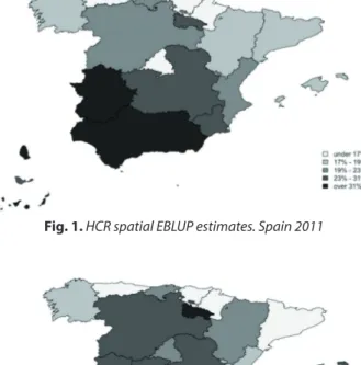
Figures 1 and 2 show the geographical distri-bution of the Spatial EBLUP estimates based on a distance approach for both HCR and S80/S20 in-dices for Spain. In the left corner of the image the islands Ceuta, Melilla and Canarias are reported widely.
It can be observed that the southern regions of Spain show the highest percentage of poor indi-viduals. The highest values are for Extremadura, Andalucía, Canarias islands and Melilla. On 1 The gain in efficiency is quantified on the following lines: for each area we calculate the ratio between the estimate of the standard error obtained by the model-based estimator and the estimate of the standard error of the direct estimate. Then, these values are averaged to get the gain in efficiency.
402 социальНо-экоНомические проблемы региоНа
the opposite, the northern ones are the richest. Here the lowest percentages of poor are found in Principado de Asturias, País Vasco, Comunidad Foral de Navarra and Cataluña. We can find again a geographical distinction also in inequality. Generally, the southern region show higher values of the S80/S20 index than the northern ones.
Comparing Figure 1 with Figure 2, we can ob-serve that, generally, those regions showing high values of HCR also present high values of S80/S20 index; this confirms that relative poverty and ine-quality are generally correlated. Exception are, on the one hand, Madrid and Balears islands, since a low HCR is accompanied by a higher level of ine-quality. On the other hand, Ceuta and Murcia are regions with a high value of poverty and very lit-tle inequality.
Considering the estimates of spatial autore-gressive coefficients it can be observed that, in both cases, this is lower when considering a dis-tance threshold approach. In fact, the disdis-tance threshold is taken to guarantee at least one link-age for each area apart from the Canarias Islands. By doing this, most linkages between areas are found in northern Spain where we find rich (une-qual) and poor (e(une-qual) regions. This can be under-stood by looking at Figure 3.
Each area is linked to its neighbours by means of black lines visible in the figure. Obviously, the neighbouring structure is influenced by the ap-proach followed by the researcher. In the figure we follow a distance-based approach, that is two ar-eas are called neighbours if the distance from each other is less than a threshold (taking as reference the centroid of each area as already explained in Section 3.1).
Figures 4 and 5 show Spatial EBLUP estimates based on a contiguity approach for HCR and S80/ S20 in Austria. It is interesting to compare here the performance of the model based estimators proposed with respect to the available sample size for each small area. It is expected that the gain in efficiency by adopting the EBLUP (or SEBLUP) es-timator will be higher for those areas where the sample size is lower or where the estimated rela-tive standard error is high. If we consider the HCR Index, in the regions of Burgenland and Carinthia the shrinkage factors are much lower than the others, meaning that most weight is attached to the regression synthetic estimator. It is not sur-prising that these areas show few sample sizes as well as a high estimated relative standard error, respectively 26 % and 18 %. Here model-based timates are much lower than direct ones. The es-timates of the spatial autoregression coefficients are moderate, and the highest gain in efficiency Fig. 1. HCR spatial EBLUP estimates. Spain 2011
Fig. 2. S80/S20 spatial EBLUP estimates. Spain 2011
Fig. 3. Distance threshold neighbours
is obtained with EBLUP. This suggests that if the spatial dependence is weak then it is better to use the traditional EBLUP. The region of Wien has the highest percentage of poor, followed by Tyrol and Karnten. The richest regions are Oberosterreich and Burgenland.
Concerning S80/S20 Index we have found that for the areas of Burgenland and Vorarlberg, the most weight is attached to the regression estimator while for Niederosterreich the most weight is given to direct estimate. This is consist-ent with the expected results as the first two ar-eas show low sample size and an estimate of the relative standard error of 14 % and 11 % respec-tively. On the contrary, the high sample size is found in Niederosterreich apart from a very low estimate of the relative standard error (4 %). The Spatial EBLUP estimator leads to a very reduced gain in efficiency. This may be due to the fact that the estimated coefficient of spatial autoregres-sion is moderate and negative, in the HCR case as well. Wien and Salzurg regions show the high-est inequality, followed by Tyrol and Steiermark. On the contrary, very low inequality is found in Oberosterreich and Burgenland.
It can be observed that here areas with high percentage of poor present also have high values of inequality and vice-versa.
4. Discussion and concluding remarks In this paper we have addressed the problem of estimating measures of well-being on their “re-gional dimension”; if fact, we have presented and compared two small area techniques, namely the cumulation and the spatial EBLUP (SEBLUP), on the basis of EU-SILC data from Austria and Spain. Both methodologies have been analysed observ-ing both advantages and drawbacks.
In general, estimates computed with the cu-mulation method show standard errors which are smaller than those computed with EBLUP or SEBLUP. The gain of pooling SILC data over three years is, therefore, relevant, and may allow re-searchers to prefer this method. However, we would
like to emphasise a point of great practical con-cern. The assessment of sampling precision of the estimates, taking into account the actual structure of the SILC sample, on which the data are based, has an essential requirement: provision of codes describing the sample in the survey micro data it-self, along with accompanying documentation de-scribing the design and the code. Inadequate (or sometimes even absence of) information on sam-ple structure in survey data files is a long-standing and persistent problem in estimation from sam-ple surveys. Unfortunately, even outstanding and highly standardised multi-country surveys such as EU-SILC have this sort of shortcomings, as un-derlined in this paper. A second drawback of the cumulation approach consists in the loss of the reference period to which the estimated meas-ures coming from the data pooling are anchored. For example, in our exercise which is the refer-ence year 2010, which is the middle year, or 2011, which is the last available year (and comparable with SEBLUP estimates)? The debate on this issue is still open, and the present paper would intend to be a new starting point in this debate.
On the other hand, when considering tech-niques such EBLUP and SEBLUP, some features of the areas for which new estimates are needed should be properly taken into account; first of all, the presence of islands or other types of geograph-ical barriers; may be that some computational procedures would fail in the presence of such a sit-uation. In such cases, the problem needs to be ad-dressed adequately. The analysis may be restricted to those areas having at least one linkage with an-other and at the same time leaving the remaining as separate cases (this is usually done in the US with Alaska and Hawaii). If the spatial dependence is not an essential feature of data, meaning an es-timated spatial autocorrelation coefficient nearly equal to zero, then a possible solution could be that of adopting the traditional EBLUP estima-tor. This estimator, by assuming the independence of the area-level random effects, does not suffer from spatial boundaries and, consequently, it is not sensitive to whether a region is an island or not. Obviously, this kind of problem can be easily overcome by following a design-based approach to small area estimation as in the case with the cu-mulation of estimates.
On the other hand, the fact that in the pre-sented results the cumulation method performs better than EBLUP and SEBLUP should be judged taking into account an additional issue: when choosing the set of regressors in the EBLUP or SEBLUP, in general researchers do not have full access to information (regressors) present at area Fig. 5. Spatial EBLUP estimates — S80/S20 Index. Austria
404 социальНо-экоНомические проблемы региоНа
level. From this point of view, National Statistical Offices could, in general, perform better, having the possibility to access a large set of regressors.
Finally, we want to highlight that in the pa-per, the estimation of the MSE of the SEBLUP es-timator has been carried out by following a pro-cedure which considers the analytical
approxima-tion of the MSE itself. Other estimators based on bootstrap procedures have been developed (see for instance [22]). We have tried to apply these pro-cedures; however, the results have been unsatis-factory, and some computational issues have been raised. Again, this is another aspect which future research should be focused on.
References
1. Atkinson, A., Cantillon, B., Marlier, E. & Nolan, B. (2002). Social Indicators: The EU and Social Inclusion. Oxford:
Oxford University Press, 24.
2. Foster, J. E., Greer, J. & Thorbecke E. (1984). A Class of Decomposable Poverty Measures. Econometrica, 52, 716–766.
3. Handerson, C. R. (1950). Estimation of Genetic Parameters. Annals of Mathematical Statistics, 21, 309–310.
4. Gosh, M. & Rao, J. N. K. (1994). Small Area Estimation: An Appraisal (with discussion). Statistical Science, 9(1),
55–93.
5. Rao, J. N. K. (2003). Small Area Estimation. Wiley, London, 24.
6. Betti, G., Gagliardi, F., Lemmi, A. & Verma, V. (2012). Sub-national Indicators of Poverty and Deprivation in Europe:
Methodology and Applications. Cambridge Journal of Regions, Economy and Society, 5(1), 149–162.
7. Fay, R. E. & Herriot, R. A. (1979). Estimates of Income for Small Places: An Application of James-Stein Procedures to
Census Data. Journal of the American Statistical Association, 74, 269–277.
8. Battese, G. E., Harter, R. M. & Fuller, W. A. (1988). An Error-components Models for Prediction of County Crop Areas
Using Survey and Satellite Data. Journal of the American Statistical Association, 83, 1–27.
9. Elbers, C., Lanjouw, J. O. & Lanjouw, P. (2003). Micro-level Estimation of Poverty and Inequality. Econometrica, 71,
335–364.
10. O’Muircheataigh, C. & Pedlow, S. (2002). Combining Samples vs. Cumulating Cases: A Comparison of Two Weighting
Strategies in NLS97. American Statistical Association. Proceedings of the Joint Statistical Meetings, 2557–2562.
11. Wells, J. E. (1998). Oversampling Through Households or Other Clusters: Comparison of Methods for Weighting the
Oversample Elements. Australian and New Zeeland Journal of Statistics, 40, 269–277.
12. Lohr, S. L. & Rao, J. N. K. (2000). Inference from Dual Frame Durveys. Journal of American Statistical Association,
95, 271–280.
13. Verma, V., Gagliardi, F. & Ferretti, C. (2013). Cumulation of Poverty Measures to Meet New Policy Needs. Advances
in Theoretical and Applied Statistics. Torelli, N. and Pesarin, F.; Bar-Hen, Avner (Eds.). XIX, Springer.
14. Verma, V., Betti, G. (2011). Taylor Linearization Sampling Errors and Design Effects for Poverty Measures and Other
Complex Statistics. Journal of Applied Statistics, 38(8), 1549–1576.
15. Verma, V., Betti, G. & Gagliardi, F. (2010). An Assessment of Survey Errors in EU-SILC. Eurostat Methodologies and
Working Papers. Eurostat, Luxembourg.
16. Pratesi, M. & Salvati, N. (2007). Small Area Estimation: The EBLUP Model Based on Spatially Correlated Random
Effects. Statistical Methods and Applications, 17(1), 113–141.
17. Verma, V. (2004). Sampling Errors and Design Effects for Poverty Measures and Other Complex Statistics. Proceedings
of the VII International Meeting Quantitative Methods for Applied Sciences: Sampling Designs for Environmental, Economic and Social Surveys: Theoretical and Practical Perspectives. Siena.
18. Cressie, N. (1993). Statistics for Spatial Data. New York: Wiley, 34.
19. Cliff, A. & Ord, J. K. (1981). Spatial Processes. Models and Applications. London: Pion, 54.
20. Banerjee, S., Carlin, B. P. & Gelfand, A. E. (2004). Hierarchical Modeling and Analysis for Spatial Data. Chapman &
Hall, New York, 78.
21. Bivand, R. S., Rubio, V. G. & Pebesma, E. J. (2008). Spatial Analysis with R. Use R!. New York: Springer, 121.
22. Molina, I., Salvati, N. & Pratesi, M. (2009). Bootsrap for Estimating the MSE of the Spatial EBLUP. Computational
Statistics, 85, 163–171.
Authors
Federico Crescenzi — Research Assistant, Department of Economics and Statistics, University of Siena (7, Piazza S.
Francesco, Siena, 53100, Italy; e-mail: [email protected]).
Gianni Betti — Associate Professor in Statistics and Economics, Department of Economics and Statistics, University of
Siena (7, Piazza S. Francesco, Siena, 53100, Italy; e-mail: [email protected]).
Francesca Gagliardi — PhD, Researcher, University of Siena (7, Piazza S. Francesco, Siena, 53100, Italy; e-mail: