Università degli Studi del Piemonte Orientale
“Amedeo Avogadro”
Dipartimento di Scienze e Innovazione Tecnologica
Dottorato di Ricerca in Chemistry&Biology
Curriculum: Energy, environmental and food sciences
XXIX ciclo a.a. 2016-2017
SSD: CHIM/01
Elemental profiling as a chemical investigation
approach: application to health studies and food
authentication
Fabio Quasso
Supervised by Prof. Emilio Marengo
Co-Supervised by Prof.ssa Elisa Robotti
PhD program co-ordinator Prof. Domenico Osella
Università degli Studi del Piemonte Orientale
“Amedeo Avogadro”
Dipartimento di Scienze e Innovazione Tecnologica
Dottorato di Ricerca in Chemistry&Biology
Curriculum: Energy, environmental and food sciences
XXIX ciclo a.a. 2016-2017
SSD: CHIM/01
Elemental profiling as a chemical investigation
approach: application to health studies and food
authentication
Fabio Quasso
Supervised by Prof. Emilio Marengo
Co-Supervised by Prof.ssa Elisa Robotti
Contents
CHAPTER 1
11.1 Introduction 1
1.1.1 Toxic Metals and Rare Earth Elements (REEs) 2
1.1.2 Elemental Profiling 19
1.1.3 Chemometrics Theory 24
1.2 Bibliography 28
CHAPTER 2
402.1 Outline of the thesis 40
CHAPTER 3
423.1 Introduction 42
3.2 Chelating Therapy for removing Metal Ions Intoxications 45
3.2.1 Materials and Methods 45
3.2.2 Results 53
3.2.3 Discussion 71
3.2.4 Conclusions 77
3.3 Plasma Proteome Profile during a Chelating Therapy 80
3.3.1 Materials and Methods 80
3.3.2 Results 84
3.3.3 Discussion 92
3.3.4 Conclusions 95
CHAPTER 4
1064.1 Introduction 106
4.1.1 The production chain of hazelnut paste 108
4.1.2 Tools for the traceability and authentication of hazelnuts 109 4.1.3 Multivariate tools for the traceability and authentication of hazelnuts 111 4.1.4 Challenges in the traceability and authentication of hazelnuts 112 4.2 Traceability and authentication study along the production chain of 113
hazelnut paste by elemental profiling
4.2.1 Materials and Methods 113
4.2.2 Results and Discussion 118
4.2.3 Conclusions 133
4.3 Authentication of hazelnut cultivars by FTIR spectroscopy 134
4.3.1 Materials and Methods 134
4.3.2 Results and Discussion 139
4.3.4 Conclusions 150 4.4 Bibliography 151
CHAPTER 5
162 5.1 Conclusions 162LIST OF PUBLICATIONS
166ACKNOWLEDGEMENTS
1671
1
CHAPTER 1
1.1 Introduction
Since the ancient times philosophers and thinkers have been questioning the structure of material. The ancient Greeks elaborated the concept of “elements” as fundamental substances which gave origin to all forms of material.
In particular, Aristotle identified 4 elements: earth, air, fire and water, which according to his studies, if combined in the right proportions, could have originated all other substances.
At the same time Democritus from Abdera theorized the existence of tiny and indivisible particles which form all the existing material; in this way the concept of atom (from the Greek gr. ἄτομος «indivisible») was introduced for the first time. Only in the XX century we have the scientific proof of the existence not only of the atom but of many atomic species, defined elements; their combination forms all the substances and so the material, too.
Once the most common chemical elements were characterized, it was necessary to classify them by using a criterium which could join them in a well-ordered way. This criterium was acknowledged for the first time by the Russian chemist Dmitri Ivanovic Mendeleev who created the Periodic Table in 1865.
In time the Periodic Table has been changed due to the finding of new elements; nowadays it is possible to differentiate several element groups.
Referring to the biological organisms, we can differentiate some elements which are fundamental for life, so extremely abundant in the organisms (C, H, O, N, S...), others which are essential at low concentrations (Se, I, Co and so on...) and others totally extraneous to the living organisms, defined as xenobiotic, which are considered harmful and very toxic (i.e. lead and mercury). There is also another particular group of elements called rare earth elements (REEs), which are considered ideal candidates
2 for geo-referencing and traceability studies in food chemstry.
1.1.1 Toxic metals and Rare Earth Elements (REEs)
Metals are the toxic agents which have been known for a long time by human beings. Differently from other toxic substances, they are neither created nor destroyed by man.
Man's action (extraction and working for industrial purposes) has influenced the state of conservation of metals in nature, and has caused a diffusion and contamination of air, water, soil and food with harmful effects on our health as a consequence.
Since the ancient times (see book Plutarch, Hippocrates 370 B.C. and so on...), the pathogen activity of some metals was known, as for example mercury and lead. Later, this definition has been diffused including elements such as cadmium, aluminum, arsenic ….
The redistribution of metals in the environment takes place naturally through the biogeochemical cycles. The rain dissolves minerals and rocks by carrying them to waterways which extract and deposit materials from the lands where they flow. Finally, the water arrives at the sea where the metals can be precipitated as sediments or can be taken up to the atmosphere where they fall down again as rains, in order to be redistributed in other areas of the Planet (figure 1) (1).
Finally, we have, through the biological cycles which include the incorporation in the food chain, the accumulation of these substances, first in the plants and then in the animals.
3
Figure 1: transport of trace elements in the environment (1).
Moreover, human activity has determined the formation of new compounds and a big increase in the world distribution of these elements.
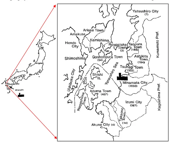
The metals come in contact with man through water, air, food and drugs. Some examples of how these elements are in relation one to each other can be the case of the disaster of Minamata and the case of the Itai-Itai disease.
Minamata case in Japan
The Minamata disease takes its name from the Japanese town of Minamata and it has been documented for the first time in May 1956 (2,3).
In 1908 the Chisso Corporation (Chisso Co. Ltd) opened a chemical factory, in Minimata, for the production of fertilizers; later, it expanded and included the production of acetylene, acetaldehyde, acetic acid, vinyl chloride and octanol. The chemical plant became the most advanced center of Japan both before and after the Second World War.
4 as catalyzer; it produces, as a residual by-product of the reaction, a small quantity of methylmercury (MeHg) (National Institute Minamata Disease) (4).
This highly toxic compound was released through the wastewaters of the factory in the Minimata Bay, from the beginning of the production in 1932 until its interruption in 1968.
The methylmercury accumulated first in the ichthyofauna and then through the food chain, among the inhabitants of the area who have a diet highly rich in fish and seafood coming from the Minamata Bay.
The geographical distribution of Minamata disease3 cases is shown in figure 2.
Figure 2: Map of Japan with Minamata Bay (3).
Among those inhabitants, the following symptoms were observed: sensory alterations (similar to those caused by glues), ataxia, dysarthria, reduction of field of
5 view, hearing ailments and tremors (5).
The exposition of the fetus to methylmercury, after the mother had eaten contaminated fish, caused much more serious consequences compared to those observed in the adults, because MeHg can cross the placenta and readily pass through the blood-brain barrier in pregnant women (6).
Cases of brain paralysis, hypoplasia of neurons of the brain cortex, growth break off and destruction of neurons could be observed (7-9).
This resulted in extreme fetal abnormalities and neurotoxicity (i.e., microcephaly, blindness, severe mental and physical developmental retardation) even among infants born from mothers with minimal symptoms (6).
In this case, the syndrome took the name of “congenital Minamata disease” (10,11). The Minamata syndrome is also known as “laughing dead”, because the patient dies with a sort of smile on his face, due to the tetanus paralysis of the face (trismus).
6 An epidemic case of Itai-Itai
Cai et al. (1995) found an epidemic form of “Itai-Itai disease” in the people of a group of villages situated on the banks of the Zhang River and the Fujang River in the Province of Jianxi in the south of China (figure 3).
They also analyzed the people who lived in the villages near the banks of the Youxian River, who did not show the same syndrome.
As the etiology of the disease was known, they evaluated the concentration of cadmium in the urine, hair and nails of ill people (villages of Zhang and Fujiang) and of healthy people (villages near Youxian); they found a high concentration of the metal in the former ones and normal concentration in the latter.
They looked for the presence of the metal in food and in the soils, eventually, they found the sources in two tungsten mines upstream of the two rivers, which
7 discharged pollutants in the waters destined to be used by farmers to irrigate agricultural fields including rice patties (12).
Figure 3: geographical map of South China (12)
Regarding the toxic heavy metals, they are further discussed independently hereafter.
1.1.1.1 Lead
Among the most toxic elements, the most widespread is lead, in fact, its presence can be found almost in any biological system. It has no physiological function in the living organisms, neither plant nor animal, and for this reason, it is toxic if it surpasses a limited amount. However, the definition of this limit, for any organism, is a problem that has no easy solution.
Children are the most affected by this metal because lead changes many functions linked to their development and, in addition, some systems of defense in children, such as the blood-brain barrier, are not completely formed and effective (13). The first people who extracted and used lead were the Egyptians, the Jews and the
8 Phoenicians (14). Thanks to its Physical-chemical characteristics, lead was widely used (i.e.to vitrify the porous surface of ceramics, to coin money etc), even though it was extremely dangerous for human health.
The ancient Romans realized about the neurotoxic effects caused by lead poisoning, in fact the saying “mad as a painter” comes from the use of “Pompeii red”, which consisted in lead oxide (15). Another example of “lead poisoning” among the ancient Romans was caused by the use of a sweetener called sapa (lead acetate) which was obtained by cooking the grape must in lead containers (16).
Lead poisoning was therefore known since the ancient times and although in the following centuries the documented cases in the literature are occasional, the pathology appears again in the documents of the XIX century, when in the period of industrialization, it reaches vast proportions. In 1920, the introduction of tetraethyl lead in fuels, caused serious damage to the public health, until it was banned in the 1980s. However, the use of tetraethyl lead was so large that it caused a big diffusion in the atmosphere, as witnessed by a 200-fold increase of lead in the ice in Greenland (17).
Lead, as an environmental pollutant, can come from several sources that can be worked or not; among those one can mention: industrial emissions (i.e. PM10), tetraethyl lead added to fuel (TEP) from 1923 to 1975, lead piping, kitchen tools, food boxes welded with lead, lead paints, mining, waste batteries, lead welding, pesticides which were used in the past in agriculture (arsenate) and contaminated food (18).
Lead is most commonly absorbed through the respiratory system, gastrointestinal tract (gastroenteric) and through transdermal means (19).
The inhaled absorption has significantly decreased since the lead compounds in fuels have been replaced by adding benzene as an antiknock, even if a new problem was created since benzene can cause leukemia. The gastroenteric absorption is not uniform in the exposed people: in particular, the affecting factors are age and diet (19).
9 Children, and all people who have a diet lacking in iron, calcium and zinc, absorb lead much more quickly and easily (20). Excretion takes place both by urine and by feces (21).
After absorption, about 90% of the lead is deposited and accumulated in the bone tissue and in the hemopoietic mallow. In this last case in particular, it interferes with the synthesis of the heme group and of the hemoglobin in the erythroid precursors (22). When the bone is remodeled also lead and likewise calcium, is redistributed in the organism (23).
Even from very low lead levels, we can notice some pathologic effects on different tissues, up to high levels showing acute intoxication.
At low lead levels, a reduction of the intellectual quotient IQ (24), hearing deficiency and some developmental and behavioral disorders in children can be observed. As the concentration increases it is possible to note some alterations of the metabolism of vitamin D (22), variations in the enzymatic expression in the erythrocytes or in their precursors, anemia due to the underproduction of hemoglobin, headache, perception of metallic flavour in the mouth, lack of appetite, constipation, abdominal colic, tremors, kidney damage with excretion of uric acid, neuropathy and encephalopathy (25).
In pregnant women, lead has a very hidden action because it is able to cross the placenta and spread in the fetal tissues (26). This can cause extremely serious malformations such as anencephaly, or spina bifida (18).
In conclusion, it is better to remember that even with concentrations which are classified as nonpathological, lead can have important toxic effects if there are other toxic elements like for example cadmium and mercury.
1.1.1.2 Mercury
Among all metallic elements, mercury is the only liquid at standard temperature conditions; it appears in two oxidation states: elemental mercury (Hg0),and mercuric
10 state (Hg2+) (27).
In the most oxidized state mercury can bind one or two carbons originating stable organic molecules, among which methylmercury (CH3Hg+) is the more toxic and
represented (28,29).
In the Middle Ages, the alchemical practices caused substantial poisoning from mercury, which was known, at that time, as ”quick silver”.
In the last century, other poisoning effects has been detected, for example, the neurotoxic effects deriving from fumes of mercury as a professional pathology of the leather tanners.
Due to its physical properties, mercury is used in the manufacturing of barometers, thermometers, hydrometers, pyrometers, UV lamps and many other special tools (30,31).
Other fields of use of Hg include the production of mirrors, gold and silver extraction, electrical rectification (32,33).
In addition, tattoo pigments, protective paints, pesticides and medicines (Thymesoral) may contain mercury (34-37).
Lastly, there is a source of iatrogenic exposure to mercury which is given by dental amalgams, used until a few years ago in dental practice. Scientific research demonstrate that it is possible to correlate excreted urine mercury after chelation therapy with the number of such amalgams (38).
As a result of human industrial activities, mercury is diffused into the environment as vapor, falling to the ground with rains, then accumulating in surface waters (37). Despite the main source of mercury vapors is the earth's crust, industrial vapors are the ones most absorbed by man as the main cause of environmental pollution (39). Indeed, it has been shown that human activities have caused a steady rise in mercury vapors over the last two centuries (40-42).
Once emitted, mercury tends to accumulate in saline and soft waters and is converted here by methanogenic bacteria into methylmercury. In this form, the metal enters the food chain bioaccumulating into larger concentrations from microorganisms to
11 predatory fish (42) (figure 4).
Figure 4: biogeochemical cycle of mercury (42)
Mercury dust and its vapors enter the body through the respiratory system, via the gastrointestinal tract and the skin (43,44).
There are two possible types of intoxication: acute and chronic. The first case causes abdominal pain, nausea, vomiting, enteric and kidney damage and death within 10 days (43,44).
Chronic intoxication, on the other hand, appears variable in symptoms, including muscle tremor, spasms at the extremities, mouth inflammation, gums, and falling teeth (43,44).
Mercury causes a pronounced lipid peroxidation of red blood cells in the hemopoietic system, probably inhibiting the activity of glutathione peroxidase (GPX) and superoxide dismutase (SOD) (45).
Several cases of interaction between the element and the immune system are reported in the literature: Hg not only has the ability of immunosuppression, but there is evidence that it can also yield immunostimulatory signals in various species,
12 including humans and rodents (46).
The formation of immunocomplexes is the cause of renal impairment of
glomerulonephritis reported on both guinea pigs (47) and humans (48).
At last, there is an observable alteration of the nervous system which manifests with irritable behavior, apprehensive states, mood swings, depression, memory disorders, learning problems, impairment of social behavior, and low intelligence quotient (49). Also, the neurotoxic effect is very relevant on adults and fetuses, as described above paragraph 1.1.1 .
1.1.1.3 Cadmium
Cadmium has a rather recent story when compared to lead and mercury: it was discovered in 1817 and it has been used in the industrial field starting from the half of the XX century. It can be used to produce batteries, fertilizers, and pigments for paints and plastic materials and in the galvanization processes. Moreover, cadmium is a residual product of extraction processes of other metals (50).
The main way cadmium is absorbed by the human body isthrough the gastroenteric system. Cadmium accumulates in cultivated plants, on polluted soils or by irrigation with water; from here, it gradually biaccumulates in the food chain (51). It can also be accumulated in a very efficient way by shellfish and mollusks (52).
Also, the cigarette smoke represents an important source of exposure: according to some estimates, a cigarette contains from 1 to 2 ug of cadmium and about 10% of it is inhaled (53).
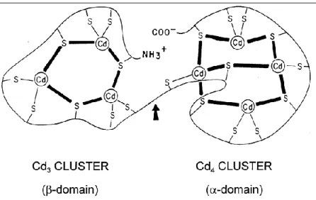
Cadmium shows strong nephrotoxicity even if the origin of this process is indirect. In fact cadmium, after its enteric absorption, goes to the liver in the bloodstream where it stimulates the synthesis of metallothionein (MT), which has the capacity to bind cadmium (figure 5). The complex Cd-MT is partly stored in the hepatocytes and partly transported to the kidneys, where it is accumulated in the lysosomes of the cells of this organ, and it causes necrosis (54). (figure 6)
13
Figure 5: Schematic structure of a metallothionein. The domain alpha coordinates four atoms of cadmium, while the domain beta joins three (54).
Depending on the exposure, a person may manifest acute or chronic intoxication. The acute toxicity by ingestion of contaminated food can cause sickness, vomiting and abdominal pains, while, if it is due to vapor inhaling, it can cause pneumonia with pulmonary edema (52).
The chronic intoxication can cause pathologies of the tubule and of the kidney glomerulus (55), damaging the metabolism of the vitamin D and of the PTH (56).
14 It is possible to have osteomalacia and osteoporosis caused by an interference with calcium metabolism, leading to bone deformation and pain which are typical of the "Itai-Itai" disease (12) (cfr paragraph 1.1.1).
Moreover, there are hypertension, cardiovascular disorders, lymphocytosis and microcytic anemia-hypochromic, emphysema, chronic pulmonary obstruction and behavior alterations and intellectual deficit.
Cadmium is classified as a category I carcinogenic by the International Agency for Research on Cancer (IARC) which is put in relation to lung cancer caused by cigarette smoke (57).
1.1.1.4 Aluminum
Aluminum is one of the elements which is the most present on our Planet because it is the third in abundance to form the earth crust. Its reactivity lets it join with +3 valence to oxygen givers such as phosphates or citrates.
It is normally present in inert forms, but in the last few decades, aluminum has become more bioavailable by acid rain which has accentuated the toxicity.
Humans can absorb aluminum from different sources, especially at home. In particular, it can be absorbed by aluminum sheets or bowls used to pack food, dishes, cutlery, coffeepots or cans made of this metal (58).
Dishes, in particular, can yield large quantities of aluminum if they are used to cook or eat acidic foods such as tomatoes and its derivatives.
Aluminum is also present in some medicines such as antacids, based on aluminium hydroxide , vaccines, which have been added with aluminum as an adjuvant, and some herbal compounds (59).
Aluminum chloride is often used in drinking water processes to flocculate impurities (58), while aluminum chloride is used in cosmetics and deodorants as an astringent (59).
15 gastroenteric, skeletal systems and on the central nervous system. In fact it interferes with the absorption of calcium, iron, and fluorides (60); in healthy patients, after the consumption of high quantities of antiacids, or in patients on dialysis, it has been shown to be a cause of osteomalacia due to its capacity to join phosphorus causing a lack of phosphates in the bones (61).
It can also cause constipation due to the intestinal inhibition of peristalsis, caused by the interference with cholinergic signals (60).
The consequences of the professional exposure to aluminum dust are mainly consisting in pulmonary fibrosis (62,63).
The capacity of aluminum to join calmodulin can cause serious consequences on the nervous system, because of the alteration of the transport tubular activity.
This last toxic activity seems to be particularly insidious and marked because it is connected to various neurologic and neurodegenerative pathologies, also depending on the age (64).
Among the most emerging ones, there are the Alzheimer Disease, the Parkinson Disease (PD), the Amyotrophic Lateral Sclerosis (ALS), the Gulf War Syndrome (GWS), Autism Spectrum Disorders (ADS), the syndrome of Guam (complex ALS-PD of Guam), the Dialysis Human Dementia Syndrome and other rare and less known diseases (64). Aluminum can substitute iron in some proteins (e.g. transferrin) (65,66), and it forms complexes with glutamate and citrate that can pass the blood-brain barrier (BBB) (67,68), causing oxidative stress in the central nervous system. Referring to what has been explained hereabove, in 1989 a mixed committee of experts FAO/OMS about food additives (JECFA) has recommended a weekly provisional and tolerable dose (PTW) of 7,0 mg/kg body weight of Al, but this limit has been modified in 2007 by reducing it to 1.0 mg/kg body weight, because they have found some potential toxic effects on the developing reproductive system and on the nervous system (69).
16
1.1.1.5 Arsenic
Even if it is not a real metal but a semi-metal, arsenic is such a diffused and toxic element that it is normally associated with the heavy metals class. In nature, it is diffused in both its oxidation states +3 and +5 which are normally forming inert mineral structures. The real danger consists in the environmental mobilization and dispersion of this element which, in this way becomes more reactive and absorbable. We can distinguish organic compounds from inorganic ones: the former can be further divided into trivalent (arsenic trioxide, sodium arsenite, arsenic trichloride) and pentavalent (arsenic pentoxide, ac. arsenic, lead and calcium arsenate) forms (70).
The latter ones are present in both trivalent and pentavalent states and in methylated form, following the bio-methylation made by the microorganisms of soil and of salt and fresh waters (71).
Arsenic is mainly dispersed in the environment by human activities, in particular as a byproduct of extraction and working of some metals as lead, copper, zinc, but also by the glass and chemical industry. There is also a specific arsenic compound, the copper acetoarsenite, also called "Paris green", added as preservative to chipboard and plywood (72).
We can’t overlook the massive use, which was done in the past, of arsenic-based pesticides and herbicides which have dispersed huge quantities of this element in the soils and waters which were intended for agriculture. Even if today these products have been banned and replaced with other herbicides and organic pesticides, arsenic is still present and can be found in a lot of food, for example, rice (73).
As any other xenobiotic elements, arsenic is metabolized by the liver and excreted by the kidneys. The hepatic metabolization in human body consists in the methylation of both the trivalent and pentavalent forms with production mono- and di- methyl arsenic (MMA and DMA). In this way, it is possible to obtain less toxic compounds which have a simpler excretion by kidney way (74).
17 In fact, the As(V) is reduced to As(III) which reacts with the S-adenosylmethionine (SAM) and is methylated to MMA and DMA (75).
Arsenic changes the functionality of mitochondrial enzymes which are involved in the cellular respiration (76); in particular, it interferes with the action of the succinate dehydrogenase and it uncouples the oxidative phosphorylation.
This causes an increase in the production of hydrogen peroxide which helps the formation of the different radical species (ROS), it causes damage to DNA and therefore potentially starts the development of cancer (74).
Moreover, the chronic exposure to low amounts of arsenic can cause serious damage to human health: ailment, fatigue, dermatitis and eczema of allergic-type and, in most serious cases, hepatic injuries followed by jaundice, cirrhosis, ascites, and also neurological damages by demyelination of nerve fibers (77).
A further danger of the chronic intoxication by arsenic is found in the mimic capacity of phosphorus which enables it to replace itself in the DNA, causing alterations in the structure and mutations. That's why IARC and EPA classified it as carcinogenic (group I), respectively in 1987 and 1988 (78).
1.1.1.6 Nickel
Nickel is a ubiquitous metal which is mainly present as an oxide, sulfide, and silicate. There are several sources of exposure, for example, cigarettes, automotive exhaust gas, and certain kinds of food as chocolate, cocoa, soy, nuts, hydrogenated oils and coffee (79).
Nickel can also be found in nickel-cadmium batteries (Ni-Cd), materials and prosthesis for dental use, costume jewelry and pigments for glass and pottery. The ordinary excretion of nickel is linked to the cysteine or other thiolic compounds (glutathione) or amino acids (histidine, aspartic acid, arginine) (80).
Most of the absorbed nickel comes from drinks and food and the concentration can change a lot, according to the geographical area, the kind of diet and the water supply
18 (81).
According to the chemical shape of the element and physiological factors, the absorption in the intestinal tract has a variation from 1% to 10%. The presence of nickel in the urine shows a recent exposure and changes a lot from day to day (82). The most clinically relevant manifestations are dermatosis, contact dermatitis, and atopic dermatitis (83). Moreover nickel exposure seems to hypersensitize the immune system, so promoting the appearance of allergic responses to various antigens (84). Finally, nickel changes enzyme functions replacing the zinc in the active sites of enzymes where it is the cofactor, by modifying the function (85). Nickel compounds are considered human carcinogens and metallic nickel is possibly a human carcinogen (86).
A last important observation concerns an evident greater sensitivity to these effects in females.
1.1.1.7 Rare Earth Elements (REE)
Rare earths are a particular group of elements considered ideal candidates for georeferencing and traceability studies on food products (87).
They are a group of 17 chemical elements, precisely scandium, yttrium and the lanthanides. Scandium and yttrium are considered rare earths because they are generally found in the same mining deposits of the lanthanides and they have similar chemical properties.
The elements belonging to the REEs are found in the earth crust in relatively high concentrations, so the name "rare earths" is not due to the abundance, but to the difficulty in extracting and separating processes.
Lanthanides have aroused particular interest, because, due to their chemical similarity, they could not be submitted to phenomena of selective fractionation in the distribution of concentration from the soil, to the plant and finally to the fruit (the REEs do not have any role in the plant physiology) (88,89).
19 transformations before commercialization (vegetable products, saffron, raw nuts, etc).
On the contrary, those products which derive from more complex processes (for example, wine), where the base product is transformed before the commercialization, can show an alteration in the REEs profile during transformation. In fact, in this case, it is necessary to consider the contribution of each process on the final REEs profile.
1.1.2 Elemental Profiling
Elemental profiling consists in the determination of all the elements contained in a sample; in line of principle, this profile includes all the elements (alkaline and alkaline-earth metals, transition metals, non-metals, lanthanides) but it is usually focused to the determination of heavy metals, potentially toxic elements (as Al, …..) and rare earths.
To date, elemental profiling is a widely used approach in basic research; it usually exploits an inductively coupled plasma (ICP) for the atomization of the sample, coupled to mass spectrometry (MS) or to optical emission (OES or ICP-AES) for the detection. ICP-MS represents a powerful tool for the quantitative determination of about 60 elements of the periodic table at trace (ppb-ppm) and ultra-trace (ppb and sometimes ppt) concentration levels.
This technique has many advantages:
• in a single analysis it allows to determine the whole elemental profile of the analyzed sample
• it allows very rapid analysis
• it is able to detect minimum concentrations distinguishing different isotopes of the same element
• it guarantees high sensitivity and reproducibility
From the scientific literature it emerges that elemental profiling focuses mainly on two different research areas: health studies and food authentication and traceability
20 studies. In the first case it is used in the health field to monitor the concentrations of elements in biological samples such as urine, plasma, blood, hair, saliva, nails, tumor tissues (90-95), with the final aim of confirming suspicions of chronic intoxication. Some recent studies relate different metals with neurodegenerative diseases such as Parkinson’s disease, Alzheimer’s disease, Amyotrophic Lateral Sclerosis (ALS) and autoimmune diseases such as multiple sclerosis (MS) (96). Studies so far have involved in particular, lead, mercury, aluminum, cadmium but a complete elemental profiling could shed on the correlation between the elements and their possible synergistic effects in influencing the onset, development and progression of these diseases, thus representing a significant step forward in their prevention and treatment. This area of research has developed in recent decades due to a strong and continuous introduction of metals and other elements into the environment. Some emblematic examples are: lead derived from petrol (97,98), mercury accumulated in fish (99,100), arsenic accumulated in rice (101). A further field of investigation has emerged in recent years concerning the dispersion of rare earth elements (REEs) in the environment due to components of computers, mobile phones and other last generation devices not properly disposed of. The replacement of mercury thermometers with thermometers using an alloy consisting of gallium, indium and tin represents a further potential source of metal pollution that is worth monitoring due to the unclear effects of these elements on human health (102,103).
The second field of research that exploits elemental profiling is food science. In this case it can be used for the characterization of food from a nutritional point of view or for traceability and authentication studies of different food products.
The elemental characterization of food can have a preventive function, both to avoid the excessive consumption of food at risk for heavy metals accumulation (e.g. mercury in tuna), and to encourage the consumption of food rich in micro and macro nutrients.
In traceability studies, elemental profiling makes it possible to relate a product to its territory. Seeds and fruits are in facts a natural site of bio-accumulation of metals
21 inside the plant. Traceability studies usually involve the determination of REEs since these elements are accumulated by plants without being fractionated: the REEs profile of the soil is thus reflected in the fruit (104). This principle is at the basis of traceability studies, focused to verify if the REEs profile remains unchanged from the soil to the final product; this principle has already been demonstrated for some short supply chains, such as that of paprika (105). For the longer production chains, the maintenance of the REEs profile is not always verified and must be evaluated from time to time (106).
On the other hand, in authentication studies for frauds identification, a link between food and territory is nor searched for but elemental profiling is used to differentiate equivalent food products from different areas without univocally binding them to the territory.
The amount of data obtained from elemental profiling does not allow a classic univariate approach to the problem, considering one variable (isotope) at a time (for example, the determination of 45 elements in 100 samples would lead to 4500 data), but rather makes it essential to apply techniques that provide a chemometric multivariate statistical treatment.
Chemometrics is a branch of analytical chemistry focused to the development and application of statistical methods for problem solving and the analysis of data in the chemical field and more generally in applied sciences.
Unlike most statistical and analytical procedures that tend to transform into univariate all the problems, even those that are intrinsically multivariate, this allows a multivariate approach to the system under investigation. Multivariate methods allow to take into account all the variables involved, making it possible to evaluate the correlations between the system descriptors and identify both synergisms and antagonisms.
For the particular application to problems treated in this PhD thesis, two main tools of multivariate analysis were exploited (107): pattern recognition methods, useful for recognizing existing structures in the data, such as groupings present in samples
22 and / or variables with a similar behavior; classification methods, able to identify mathematical models for the differentiation of the samples in different classes. Pattern recognition tools are unsupervised methods, i.e methods where no a priori hypotheses are formulated on how the samples are grouped, aimed to display data in a compact and easily readable way, so that the homogeneous groups can be recognized within the sample set. Among the unsupervised techniques, Principal Components Analysis (PCA) is undoubtedly the most widespread, together to cluster analysis (CA).
Classification tools are instead supervised methods that, unlike the previous ones, are based on the assumption that the existence of groups or classes is already known and defined. This condition may derive from the fact that the samples are conceptually separated in theoretical classes or may derive from a previous identification of groups of samples by PCA or CA. Classification methods are aimed to identify the variables mostly responsible for the separation of the classes of samples, i.e. the identification of candidate markers. Each class is then described by a mathematical model that can be applied to unknown samples to evaluate their belonging to one class or another. Among the classification mostly exploited in traceability and authentication studies, we find Linear Discriminant Analysis (LDA) (108,109), Principal Component Analysis – Discriminant Analysis (PCA-DA) (108, 109), Partial Least Squares – Discriminant Analysis (PLS-DA) (108,109) and Soft Independent Model of Class Analogy (SIMCA) (108,109).
In literature, several papers are present about traceability and authentication studies exploiting multivariate statistics on elemental profiling For example, Aceto et al. (106) studied the possibility to use lanthanides (La, Ce, Pr, Nd, Sm, Eu, Gd, Tb, Dy, Ho, Er, Tm, Yb, Lu) as chemical markers in a traceability study about the Moscato d'Asti wine production chain; soils, grapes and musts were analyzed by ICP-MS. The effect played by oenological practices on the REEs distribution was evaluated. In this work, PCA and CA were applied and proved that the lanthanides fingerprint is kept unaltered in the passage from soils to grapes and musts; alterations are instead
23 observed on the wine after clarification treatments using bentonites.
Another paper Bontempo et al. (110) reports the possibility of tracing the geographical origin, in tomato and derivatives along the production chain (juice, passata and paste) by Isotope Ratio Mass Spectrometry, Inductively Coupled Plasma Mass Spectrometry and Ion Chromatography. The samples used in this study came from three different Italian regions (Piedmont, Emilia Romagna, and Apulia). The traceability of these products was demonstrated: excellent discrimination among products from the three regions was achieved by applying linear discriminant analysis (LDA) on 17 parameters (Gd, La, Tl, Eu, Cs, Ni, Cr, Co, d34S, d15N, Cd, K, Mg, d13C, Mo, Rb and U).
Another study is about the Red Onion of Tropea (Calabria, Italy), an Italian product of excellence, registered on the European list of "Denominations of Origin and Protected Geographical Indications" on March 28, 2008 with Reg. CE n. 284/2008 of the Commission (111); in this study, Furia et al. (112) developed a reliable classification model of onion samples in groups corresponding to “Tropea” and “non-Tropea” categories. The concentrations of 25 elements (Al, Ba, Ca, Cd, Ce, Cr, Dy, Eu, Fe, Ga, Gd, Ho, La, Mg, Mn, Na, Nd, Ni, Pr, Rb, Sm, Sr, Tl, Y, and Zn) in onion samples with PGI brand (120) and onion samples not cultivated following the production regulations (80) were analyzed by ICP-MS. Different chemometric approaches were tested: LDA SIMCA, and back-propagation artificial neural networks (BP-ANN). Satisfactory results (prediction ability >90%) were obtained. Finally, Spiros et al.(113) discriminated ‘‘Fava Santorinis’’ from other yellow split peas, by four classification methods applied to REEs and trace elements determination by ICP-MS. In this paper, orthogonal projection analysis (OPA), Mahalanobis distance (MD), PLS-DA and k nearest neighbors (KNN) were applied. OPA provided the best results 100% accuracy).
When multivariate tools are applied to elemental profiling, particular attention must be paid to data pretreatment. Since the absolute concentrations of the elements usually decreases along the production chain, their use in traceability and
24 authentication studies is unfeasible. Elemental concentrations are usually normalized, that is scaled with respect to a reference analyte that has to remain unchanged in the samples under investigation.
As for the elements to be used as normalizing factors, studies are present in literature that use as normalizing factors different elements such as strontium, barium, lanthanum or rubidium. The choice is usually driven by the fact that the chosen element must remain unchanged within the samples under analysis. In other cases, the most adequate standardization factor needs to be identified in order to solve the problem.
1.1.3 Chemometrics Theory
Hereafter, the multivariate statistical methods used in this Ph.D. thesis will be briefly presented.
1.1.3.1 Data pretreatment
When multivariate techniques are applied, data pretreatment is usually necessary to provide reliable results. The most exploited scaling technique is autoscaling, consisting in a two steps procedure: data are first mean centered so that the new average value for each variable equals 0; then, the data are normalized by the standard deviation of each variable independently, so that the new variables have all unit variance. This scaling is useful to provide variables accounting for the same amount of information, thus eliminating scale effects.
Here, autoscaling was always applied when applying PCA or other multivariate statistical techniques.
When multivariate tools are applied in traceability studies based on elemental profiling, it is preferable to deal with ratios rather than with the absolute concentration of the elements since this last one naturally decreases passing from soil to the fruit and so on along the production chain.
25 be used as a normalizing factor, by the expression:
𝑥𝑖,𝑗′ = 𝑥𝑖,𝑗
𝑥𝑖,𝑘 i≠k (1)
where 𝑥𝑖,𝑗′ is the normalized value for the i-th sample and the j-th analyte, 𝑥
𝑖,𝑗 is the
concentration level of the i-th sample and the j-th analyte and 𝑥𝑖,𝑘 is the concentration level of the i-th sample and the k-th analyte (where i≠k).
1.1.3.2 Statistical Analysis: Principal Component Analysis (PCA)
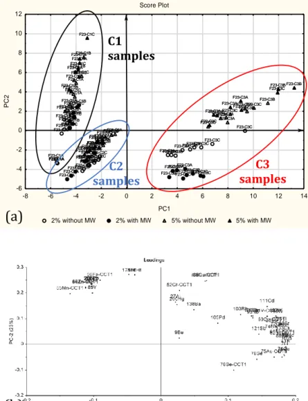
PCA (108,109) is a multivariate statistical method allowing the representation of the objects (samples), described by the original variables (metal concentrations), in a new reference system characterized by new variables called Principal Components (PCs). The PCs are calculated hierarchically: the first PC accounts for the maximum amount of the original variance, while subsequent PCs account for the maximum residual variance, so that systematic variations are explained in the first PCs, while experimental noise and random variations are contained in the last ones. Each PC is a linear combination of the original variables and they are orthogonal to each other, thus accounting for independent sources of information. PCA provides two main tools for data analysis: the scores, representing the co-ordinates of the samples in the space given by the PCs; the loadings, representing the coefficients of the linear combination describing each PC, i.e. the weights of the original variables on each PC. The scores allow the identification of groups of samples showing similar (samples close one to the other in the graph) or different (samples far from each other) behaviors. By looking at the corresponding loading plot, it is possible to identify the variables that are responsible for the similar or different behaviors detected for the samples in the score plot. PCA was applied here after varimax rotation of the most relevant PCs; this treatment allows the maximization of the variances of all the original variables on each PC (108,109).
26
1.1.3.3 Partial Least Squares – Discriminant Analysis (PLS-DA)
Partial Least Square (PLS) (108,109) is a multivariate regression method establishing a relationship between one or more dependent variables (Y) and a group of descriptors (X). X and Y variables are modeled simultaneously, to find the latent variables (LVs) in X that will predict the LVs in Y. When a large number of descriptors (X variables) are present, or a large experimental error is expected, it can be quite difficult to obtain a final model with a suitable predictive ability. In these cases, techniques for variable selection are usually exploited. Here, a backward elimination (BE) strategy was applied, eliminating one variable at a time, according to the minimum error in cross-validation; variables are eliminated according to the smallest importance (114). PLS was originally proposed to model continuous responses, but it can be applied also for classification purposes by establishing an appropriate Y response matrix related to the belonging of each sample to a class. The regression is then carried out between the X-block variables (here the elemental) and the Y just established. This application for classification purposes is called PLS-DA (115,116). In this case, where three classes are present, three binary variables were added to the Y matrix, coded so that +1 means that the sample belongs to a certain cultivar corresponding to the specific column, while -1 means that the sample does not belong to the class associated to the specific column.
1.1.3.4 Principal Component Analysis – Linear Discriminant Analysis (PCA-LDA)
LDA (117-119) is a Bayesian classification method providing the classification of the objects taking into consideration at the same time the multivariate structure of the data. Each object is classified in a particular class g if the so-called discriminant score Dg is minimum:
𝐷𝑔(𝑥𝑖) = (𝑥𝑖− 𝑥̅𝑔) 𝑇
𝑆𝑔−1(𝑥𝑖 − 𝑥̅𝑔) + ln|𝑆𝑔| − 2 ln 𝑃𝑔 (5)
where, Sg is the covariance matrix of class g; 𝑥̅𝑔 is the centroid of class g, xi is the
27
Sg is approximated with the pooled (between the classes) covariance matrix; this corresponds to considering all the classes as having a common shape (i.e., the average, weighted over the degrees of freedom, of the shape of the present classes). The variables contained in the LDA model discriminating the classes can be chosen by a stepwise algorithm, selecting iteratively the most discriminating variables. Here, a forward selection (FS) procedure was applied: at each iteration, the variable guaranteeing the best Non-Error-Rate (NER%) in cross-validation was added to the final model. FS-LDA was applied to the principal components rather than to the original variables. The loadings of the PCs allow the calculation of the final weight of each original variable on the LDA model built on the PCs.
1.1.3.5 Evaluation of the classification performances
The classification performances can be evaluated both in fitting and cross-validation by the calculation of several indexes. The confusion matrix is a matrix reporting the true classes on the rows and the assigned classes on the columns. Given G classes, each element nkl represents the number of samples belonging to class k and assigned
to class l. The diagonal values ngg, corresponding to each g-th class, are the correct
assignments (i.e. samples correctly assigned to a class), while the extra-diagonal elements correspond to the miss-classifications (i.e. samples of a class erroneously attributed to another class). The sum of each row is the number of samples belonging to the corresponding g-th class (ng), while the sum of each column is the number of
samples assigned to the corresponding g-th class (n’g). All the indexes related to the
classification performances can be calculated starting from the confusion matrix:
Precision is the capability of a classification model to not include samples of other
classes in the considered class. For each class g, it is calculated as the percentage ratio of the number of samples correctly assigned to class g (ngg) and the total number
of samples assigned to class g (n’g).
28 belonging to the g-th class. It is calculated as the percentage ratio of samples correctly assigned to class g (ngg) and the total number of samples belonging to class
g (ng).
Specificity is the capability of the g-th class to reject the samples of all the other
classes. It is calculated as:
𝑆𝑝𝑔 =∑𝐺𝑘=1(𝑛𝑘′−𝑛𝑔𝑘)
𝑛−𝑛𝑔 ∗ 100 for k≠g (3)
where G is the number of classes and n'k is the total number of samples assigned to
class k:
𝑛′𝑘 = ∑𝐺𝑔=1𝑛𝑔𝑘 (4)
Accuracy is the percentage ratio of the overall correctly assigned samples,
considering all the classes contemporarily.
The Non Error Rate (NER%) is the average of the class sensitivities, while the Error
Rate (ER%) is the complement to 100% of the NER%.
1.2 Bibliography
1. Beijer K., Jernelöv A. ( 1986) Sources, transport and transformation of metals in the environment In: Friberg L, Nordberg GF and Vouk VB (eds) Handbook on the Toxicology of Metals. Amsterdam: Elsevier, 68-84.
2. Eto K. (1997) Pathology of Minamata Disease. Toxicol. Pathol. 25, 6: 614-623.
3. Harada M. (1995) Minamata Disease: Methylmercury Poisoning in Japan Caused by Environmental Pollution. Crit Rev Toxicol. 25(1):1-24.
4. NIMD: Report of the Social Scientific Study Group on Minamata Disease, In the Hope of Avoiding Repetition of a Tragedy of Minamata Disease, National Institute for Minamata Disease, p. 13.
5. Kumamoto University Study Group (1968). Pathology of Minamata desease. In: Minamata Disease, M Kutsuna (ed). Shuhan, Kumamoto, Japan, pp.
141-29 252.
6. Crammer M., Gilbert S., Crammer J. (1996) Neurotoxicity of mercury-indicators and effects of low-level exposure overview. Neurotoxicology. 17 (1): 9-14.
7. Takeuchi T., Kambra T., Morikawa N., Matsumoto H., Shiraishi Y., and Ito H. (1959) Pathologic observations of the Minamata disease. Acta Pathol. Jpn. 9(suppl.): 769-783.
8. Matsumoto H., Koya G., and Takeuchi T. (1965) Fetal Minamata disease: A neuropathological study of two cases of intrauterine intoxication by methylmercury compound. J. Neuropathol. Exp. Neurol. 24: 563-574. 9. Choi B.H., Lapham L.W., Amin-zaki L., and Saleem T. (1978) Abnormal
neuronal migration, deranged cerebral cortical organization, and diffuse white matter astrocytosis of human fetal brain: A major effect of methylmercury poisoning in utero. J. Neuropathol. Exp. Neurol. 37: 719-733. 10. Takeuchi T. (1977) Pathology of fetal Minamata disease. Pediatrician 6:
69-87.
11. Takeuchi T., Matsumoto H., and Koya G. (1964) A pathological study of fetal Minamata disease diagnosed clinically as so-called infantile cerebral palsy. Adv. Neurol. 8(4): 145-161 (in Japanese).
12. Cai S., Yue L., Shang Q., Nordberg G. (1995) Cadmium exposure among residents in an area contaminated by irrigation water in China. Bull World Health Organization. 73, 359–367.
13. Needleman H.L., Schell A., Bellinger D. et al. (1990) Long-term effects of childhood exposure to lead at low doses: An eleven-year follow –up report. N Engl J Med. 322:82-88.
14. Woolley D.E. (1984) A perspective of lead poisoning in antiquity and the present. Neurotoxicology. 5(3):353-61.
15. Gilfillan S.C. (1965) Lead poisoning and the fall of Rome. J Occup Med. 7:53-60.
30 16. Nriagu J.O. (1983) Occupational exposure to lead in ancient times. Sci Total
Environ. 31(2):105-16.
17. Ng A., Patterson C. (1981) Natural concentrations of lead in ancient Arctic and Antarctic ice. Geochimica et Cosmochimica Acta. 45,11, 2109-2121. 18. Ugazio G. Compendio di Patologia Ambientale. Edizione Minerva Medica
pp 11-24 (2008).
19. https://www.atsdr.cdc.gov/csem/lead/docs/CSEM-Lead_toxicity_508.pdf 20. Bruening K., Kemp F.W., Simone N., Holding Y., Louria D.B., Bogden J.D.
(1999) Dietary calcium intakes of urban children at risk of lead poisoning. Environ Health Perspect. 107:431-435.
21. Skerfving S., Gerhardsson L., Schutz A., Stromberg U. (1998) Lead— biological monitoring of exposure and effects. J Trace Elem Exp Med. 11:289–301.
22. Goyer R.A., Rhyne B.C. (1973) Pathological effects of lead. Int Rev Exp Pathol. 12:1–77.
23. Pounds J.G., Long G.J., Rosen J.F. (1991) Cellular and molecular toxicity of lead in bone. Environ Health Perspect. 91:17–32.
24. Needleman H.L., Schell A., Bellinger D. et al. (1990) Long-term effects of
childhood exposure to lead at low doses: An eleven-year follow –up report. N Engl J Med. 322:82-88.
25. Goyer R.A. (1990) Lead toxicity: From overt to subclinical to subtle health effects. Environ Health Perspect. 86:177–181.
26. Gundacker C., Hengstschläger M. (2012) The role of the placenta in fetal exposure to heavy metals. Wien Med Wochenschr. 162(9-10):201-6.
27. Kim M.K., Zoh K.D. (2012) Fate and Transport of Mercury in Environmental Media and Human Exposure. J Prev Med Public Health. 45:335-343.
28. Tchounwou P.B., Yedjou C.G., Patlolla A.K., and Sutton D.J. (2012) Heavy Metals Toxicity and the Environment. EXS. 101: 133–164.
31 Med Interne. 32(7):416-24.
30. Clarkson T.W. et al. (2003) The toxicology of mercury – current exposures and clinical manifestations. N Engl J Med. 349: 1731.
31. http://www.who.int/ceh/capacity/Mercury.pdf
32. Bengtsson U.G.,Hylander L.D. (2017) Increased mercury emissions from modern dental amalgams. Biometals. 30:277–283.
33. Clarkson T.W., Vyas J.B., and Ballatori N. (2007) Mechanisms of Mercury Disposition in the Body. American Journal Of Industrial Medicine. 50:757– 764.
34. Thum C.K., Biswas A. (2015) Inflammatory complications related to tattooing: a histopathological approach based on pattern analysis. Am J Dermatopathol. 37(1):54-66.
35. Rodrigues J., Branco V., Luc J., Holmgren A., Carvalho A. (2015) Toxicological effects of thiomersal and ethylmercury: Inhibition of the thioredoxin system and NADP+-dependent dehydrogenases of the pentose phosphate pathway. Toxicology and Applied Pharmacology. 286, 216–223. 36. Tchounwou P.B., Ayensu W.K., Ninashvilli N., Sutton D. (2003)
Environmental exposures to mercury and its toxicopathologic implications for public health. Environ Toxicol. 18:149–175.
37. Maqboola F., Niaza K, Hassana F.I., Khana F., and Abdollahi M. (2017) Immunotoxicity of mercury: Pathological and toxicological effects. Journal of Environmental Science and Health, Part C. Vol. 35, No. 1, 29-46.
38. Aposhian H.V., Bruce D.C., Alter W., et al. (1992) Urinary mercury after administration of 2, 3-dimercaptopropane-1-sulfonic acid: correlation with dental amalgam score. FASEB J. 6:2472-2476.
39. Goldman L.R., Shannon M.W. and the Committee on Environmental Health. Technical Report: Mercury in the Environment: Implications for Pediatricians. Pediatrics 2001;108;197.
32 40. Monteiro L.R., Furness R.W. (1997) Accelerated increase in mercury contamination in north Atlantic mesopelagic food chains as indicated by time series of seabird feathers. Environmental Toxicology and Chem. 16, 2489– 2493.
41. United Nations Environment Programme. The global atmospheric mercury assessment: sources, emissions and transport. Geneva: United Nations Environment Programme; 2008, p. 13-62.
42. Kim M.K., Zoh K.D. (2012) Fate and Transport of Mercury in Environmental Media and Human Exposure. J Prev Med Public Health. 45:335-343.
43. Park J.D. and Zheng W. (2012) Human Exposure and Health Effects of Inorganic and Elemental Mercury. J Prev Med Public Health. 45(6): 344– 352.
44. https://www.atsdr.cdc.gov/mmg/mmg.asp?id=106&tid=24
45. Bulat P., Dujić I., Potkonjak B., Vidaković A. (1998) Activity of glutathione peroxidase and superoxide dismutase in workers occupationally exposed to mercury. Int Arch Occup Environ Health. 71 Suppl:S37-9.
46. Pollard K.M., Pearson D.L., Hultman P., Hildebrandt B., Kono D.H. (1999) Lupus-prone mice as models to study xenobiotic-induced acceleration of systemic autoimmunity. Environ Health Perspect. 107:729.
47. Henry G.A., Jarnot B.M., Steinhoff M.M. et al. (1998) Mercury-induced renal autoimmunity in the MAXX rat. Clinical Immunology and Immunopathology. Vol 49:187–203.
48. Pelletier L., Druet P. (1995) Immunotoxicology of metals. Toxicology of Metals Handbook of Experimental Pharmacology. Vol 115, pp 77-92. 49. Stein J., Schettler T., Wallinga D., Valenti M. (2002) In harm’s way: toxic
threats to child development. J. Dev. Behav. Pediatr. 23, pp. S13-S22. 50. ATSDR: Cadmium (Update). Washington, DC: U.S. Department of Health
33 51. Smith S.W. (2013) The Role of Chelation in the Treatment of Other Metal
Poisonings J. Med. Toxicol. 9:355–369.
52. https://www.atsdr.cdc.gov/substances/toxsubstance.asp?toxid=15 53. http://www.cdc.gov/niosh/docs/1970/76-192.html.
54. Klaassen C.D., Liu J., Choudhuri S. (1999) Metallothionein: an intracellular protein to protect against cadmium toxicity. Annu Rev Pharmacol Toxicol. 39:267-94.
55. Buchet J.P., Lauwerys R., Roels H. et al. (1990) Renal effects of cadmium body burden of the general population. Lancet. 336:699-702.
56. Friberg L., Eliner C.F., Kjellstrom T., et al. Cadmium and Health: A Toxicological and Epidemiological Appraisal. Vol II. Effects and Respose. Boca Raton, FL: CRC Press, 1986, pp 1-307.
57. IARC: Monographs on the Evaluation of Carcinogenic Risks to Humans. Vol 58. Beryllium, Cadmium, Mercury, and Exposures in the Glass Manufacturing Industry. Lyons, France: IARC(1993).
58. Fekete V., Vandevijvere S., Bolle F., Van Loco J. (2013) Estimation of dietary aluminum exposure of the Belgian adult population: evaluation of contribution of food and kitchenware. Food Chem. Toxicol. 55, pp. 602-608. 59. Bondy S.C. (2015) Low levels of aluminum can lead to behavioral and morphological changes associated with Alzheimer’s disease and age-related neurodegeneration. Neurotoxicology, 52, pp. 222-229.
60. Exley C., Burgess E., Day J.P., Jeffery E.H., Melethil S., Yokel R.A. (1996) Aluminum toxicokinetics. J Toxicol Environ Health. 48: 569–584.
61. P.C., Couttenye M.M., De Broe M.E. (1996) Diagnosis and treatment of aluminium bone disease. Nephrol Dial Transplant. 11(Suppl 3) 74–79. 62. Riihimaki V., Aitio A. (2012) Occupational exposure to aluminum and its
biomonitoring in perspective. Crit Rev Toxicol. 42(10) 827–853.
63. Malo J.L., Vandenplas O. (2011) Definitions and classification of work-related asthma. Immunol Allergy Clin N Am. 31(4):645–662.
34 64. Shaw C.A., Tomljenovic L. (2013) Aluminum in the central nervous system (CNS): toxicity in humans and animals, vaccine adjuvants, and autoimmunity. Immunol Res. 56(2-3):304-16.
65. Trapp G.A. (1983) Plasma aluminium is bound to transferrin. Life Sci. 33:311-306.
66. Murko S., Scancar J., Milacic R. (2011) Rapid fractionation of Al in human serum by the use of the HiTrap desalting size exclusion column with ICP-MS detection. J Anal At Spectrom. 26:86-93.
67. Deloncle R., Guillard O., Clanet F., Courtois P., Piriou A. (1990) Aluminum transfer as glutamate complex through blood-brain barrier. Possible implication in dialysis encephalopathy. Biol Trace Elem Res. 25(1):39-45. 68. Canales J.J., Corbalán R., Montoliu C., Llansola M., Monfort P., Erceg S.,
Hernandez-Viadel M., Felipo V. (2001) Aluminium impairs the glutamate-nitric oxide-cGMP pathway in cultured neurons and in rat brain in vivo: molecular mechanisms and implications for neuropathology. J Inorg Biochem. 87(1-2):63-69.
69. World Health Organization, Safety Evaluation of Certain Food Additives and
Contaminants. Food Additive Series: 58, 2007
http://whqlibdoc.who.int/trs/WHOTRS940eng.pdf.
70. Crisponi G., Nurchi V.M., Crespo-Alonso M., Toso L. (2012) Chelating agents for metal intoxication. Curr Med Chem. 19(17):2794-815.
71. Lomax C., Liu W.J., Wu L. , Xue K., Xiong J., Zhou J. , McGrath S.P., Meharg A.A., Miller A.J. and Zhao F.J. (2012) Methylated arsenic species in plants originate from soil microorganisms. New Phytologist. 193: 665–672. 72. Goyer R.A. and Clarkson T.W. TOXIC EFFECTS OF METALS. CHAPTER
23. Casarett & Doull's Essentials of Toxicology, 2e Klaassen CD, Watkins JB.
35 73. Awasthi S., Chauhan R., Srivastava S., Tripathi R.D. (2017) The journey of arsenic from soil to Grain in Rice. Frontiers in Plant Science. 8, 20, Article number 1007.
74. NRC: Arsenic in Drinking Water. Washington, DC: National Academy Press, 1999, pp1-308.
75. Bentley R., Chasteen T.G. (2002) Microbial Methylation of Metalloids: Arsenic, Antimony, and Bismuth. Microbiol Mol Biol Rev. 66(2): 250–271. 76. Brown M.M., Rhyne B.C., Goyer R.A. & Fowler B.A. (1976) Intracellular
effects of chronic arsenic administration on renal proximal tubule cells. Journal of Toxicology and Environmental Health. Volume 1, Issue 3. 77. http://www.atsdr.cdc.gov/substances/toxsubstance.asp?toxid=3
78. IARC Working Group on the Evaluation of Carcinogenic Risks to Humans. Arsenic, metals, fibres, and dusts. IARC Monogr Eval Carcinog Risks Hum. 2012;100(Pt C):11-465.
79. Medical and Biological Effects of Environmental Pollutants: Nickel, Nat. Acad. Sci, Washington DC,1975.
80. Sunderman F.W. (1989) Mechanisms of nickel carcinogenesis. Scand J Work Environ Health. 15:1–12.
81. Ambient Water Quality Criteria for Nickel, US EPA NTIS, Springfield, VA. Publ No. PB81-117715,1980.
82. https://www.atsdr.cdc.gov/toxprofiles/tp.asp?id=245&tid=44
83. Bocca B., Forte G., Pino A. and Alimonti A. (2013) Heavy metals in powder-based cosmetics quantified by ICP-MS: an approach for estimating measurement uncertainty. Anal. Methods. 5, 402-408
84. Yoshioka Y., Kuroda E., Hirai T., Tsutsumi Y. and Ishii K.J. (2017) Allergic Responses Induced by the Immunomodulatory Effects of Nanomaterials upon Skin. Exposure Front. Immunol. 8, 189.
85. Foster A.W., Osman D., and Robinson N.J. (2014) Metal Preferences and Metallation. J Biol Chem. 289(41): 28095–28103.
36 86. IARC, International Agency for Research on Cancer, 2012. Arsenic, metals,
fibres, and dusts. Vol. 100 C, IARC, Lyon, France.
87. Aceto M. (2016) The Use of ICP-MS in Food Traceability (Book Chapter) Advances in Food Traceability Techniques and Technologies: Improving Quality Throughout the Food Chain. pp. 137-164.
88. Tyler G. (2004) Rare earth elements in soil and plant systems: a review. Plant Soil 267, 191–206.
89. Liang T., Ding S., Song W., Chong Z., Zhang C., Li H. (2008) A review of fractionations of rare earth elements in plants. Journal of Rare Earths 26, 7– 15.
90. Bocca B., Mattei D., Pino A., Alimonti A. (2011) Monitoring of environmental metals in human blood: The need for data validation. Current Analytical Chemistry. Volume 7, Issue 4, 269-276.
91. Goulle J-P., Mahieu L., Castermant J., Neveu N., Bonneau L., Laine G., Bouige D., Lacroix C. (2005) Metal and metalloid multi-elementary ICP-MS validation in whole blood, plasma, urine and hair reference values. Forensic Sci. Int., 153, 39–44.
92. Chirila E., Draghici C. (2011 ) Analytical Approaches for Sampling and Sample Preparation for Heavy Metals Analysis in Biological Materials. NATO Science for Peace and Security Series C: Environmental Security. 1, pp. 129-143.
93. Hussein W.F., Njue W., Murungi J., Wanjau R., (2008) Use of human nails as bio-indicators of heavy metals environmental exposure among school age children in Kenya, Sci. Total Environ. 393, 376–384.
94. Alimonti A., Bocca B., Mattei D., Lamazza A., Fiori E., De Ercole M., Pino A., Forte G. (2009) Composition of essential and non-essential elements in tissues and body fluids of healthy subjects and patients with colorectal polyps. International Journal of Environment and Health. 3,2, 2009, 224-237.
37 95. Chung H.K., Nam J.S., Ahn C.W., Lee Y.S., Kim K.R. (2016) Some Elements in Thyroid Tissue are Associated with More Advanced Stage of Thyroid Cancer in Korean Women Biological Trace Element Research. 171(1), pp. 54-62.
96. Fulgenzi A., Vietti D., Ferrero M.E. (2017) Chronic toxic-metal poisoning and neurodegenerative diseases. International Journal of Current Research. 9,09, pp.57899-57909.
97. Caplun E.B.A., Petit D., Picciotto D.E. (1984) Lead in petrol. Endeavour. 8, 3, 135-144.
98. http://www.who.int/bulletin/archives/80(10)768.pdf
99. Carneiro M.F., Grotto D., Barbosa F. (2014) Inorganic and methylmercury levels in plasma are differentially associated with age, gender, and oxidative stress markers in a population exposed to mercury through fish consumption. J Toxicol Environ Health A. 77(1-3):69-79.
100. EFSA Scientific Committee, 2015. Statement on the benefits of fish / seafood consumption compared to the risks of methylmercury in fish / seafood. EFSA Journal, 13(1), p.3982.
101. Islam S., Rahman M.M., Islam M.R., Naidu R. (2016) Arsenic accumulation in rice: Consequences of rice genotypes and management practices to reduce human health risk. Environment International 96 139–155.
102. Nabi S. (2014) Toxic Effects of Mercury | | Springer 2014 Chapter 2, 9-14. 103. Geratherm Medical AG (2011, July 20). Galinstan Safety Data Sheet
[Online]. Available: http://www.rgmd.com/msds/msds.pdf
104. Liang, T., Ding, S., Song, W., Chong, Z., Zhang, C., Li, H., 2008. A review of fractionations of rare earth elements in plants. Journal of Rare Earths 26, 7–15.
105. Brunner M., Katona R., Stefanka Z., Prohaska T. (2010) Determination of the geographical origin of processed spice using multielement and isotopic pattern on the example of Szegedi paprika. European Food research and
38 Technology. 231(4), 623-634.
106. Aceto M, Robotti E., Oddone m., Baldizzone M., Bonifacino g., Bezzo G., Di Stefano R., Gosetti F., Mazzucco E., Manfredi M., Marengo E. (2013) A traceability study on the Moscato wine chain. Food Chemistry. 138, 1914– 1922.
107. Gonzalvez A., Armenta S., de la Guardia M. (2009) Trace-element composition and stable-isotope ratio for discrimination of foods with Protected Designation of Origin. Trends in Analytical Chemistry. 28, 11, 1295-1311.
108. Massart D.L., Vandeginste B.G.M., Deming S.M., Michotte Y., Kaufman L. (1988) Chemometrics: A textbook. Amsterdam: Elsevier.
109. Vandeginste B.G.M., Massart D.L., Buydens L.M.C., Yong S. De, Lewi P.J., Smeyers-Verbeke J. Handbook of Chemometrics and Qualimetrics: Part B. Amsterdam: Elsevier, 1998.
110. Bontempo L., Camin F., Manzocco L., Nicolini G., Wehrens R., Ziller L., Larcher R. (2011) Traceability along the production chain of Italian tomato products on the basis of stable isotopes and mineral composition. Rapid Commun. Mass Spectrom. 25, 899–909.
111. Commission Regulation (EC) No 284/2008 of 27 March 2008 registering certain names in the Register of protected designations of origin and protected geographical indications Lingot du Nord (PGI), Cipolla Rossa di Tropea Calabria (PGI), Marrone di Roccadaspide (PGI).
112. Furia E., Naccarato A., Sindona G., Stabile G., Tagarelli A. (2011) Multielement Fingerprinting as a Tool in Origin Authentication of PGI Food Products: Tropea Red Onion. J. Agric. Food Chem. 59, 8450–8457.
113. Drivelos S.A., Higgins K., Kalivas J.H., Haroutounian S.A., Georgiou C.A. (2014) Data fusion for food authentication. Combining rare earth elements and trace metals to discriminate ‘‘Fava Santorinis’’ from other yellow split peas using chemometric tools.Food Chemistry. 165, 316–322.