PAPER
An optomechanical heat engine with feedback-controlled
in-loop light
Najmeh Etehadi Abari1,2
, Giulia Vittoria De Angelis1
, Stefano Zippilli1
and David Vitali1,3,4
1 School of Science and Technology, Physics Division, University of Camerino, I-62032, Camerino(MC), Italy 2 Department of Physics, Faculty of Science, University of Isfahan, Hezar Jerib, 81746-73441, Isfahan, Iran 3 INFN, Sezione di Perugia, I-06123, Perugia, Italy
4 CNR-INO, Largo Enrico Fermi 6, I-50125, Firenze, Italy
E-mail:[email protected]
Keywords: optomechanics, quantum heat engine, feedback
Abstract
The dissipative properties of an optical cavity can be effectively controlled by placing it in a feedback
loop where the light at the cavity output is detected and the corresponding signal is used to modulate
the amplitude of a laser
field which drives the cavity itself. Here we show that this effect can be
exploited to improve the performance of an optomechanical heat engine which makes use of polariton
excitations as working
fluid. In particular we demonstrate that, by employing a positive feedback close
to the instability threshold, it is possible to operate this engine also under parameters regimes which
are not usable without feedback, and which may significantly ease the practical implementation of this
device.
1. Introduction
Heat engines convert thermal energy into work. A quantum heat engine uses a quantum system as workingfluid. The practical realization of these devices is interesting as platforms for the experimental investigation of the thermodynamics of the quantum world and of non-equilibrium systems[1,2].
Optomechanics[3] describes systems, which range from the nanoscale to macroscopic sizes, where the interaction between light and mechanical objects is exploited for enhanced metrology[4], and to explore the limits of quantum physics[5,6]. Thermal machines based on optomechanical systems have been proposed and analysed in different configurations [7–15]. A specific example [7–9] makes use of hybridized polariton
excitations as workingfluid. This engine works in the strong optomechanical coupling regime where the normal modes of the system are superpositions of optical and mechanical excitations. This regime is in general not easily achievable and in some cases is inhibited by detrimental nonlinear processes, such as optical bistability or thermorefractive effects, which hamper the ability to carefully control the coupled dynamics of the systems. It has been shown[16] that feedback-controlled light [16–19] can be employed to significantly ease the onset of strong coupling in an optomechanical system. This suggests[20] that the feedback analysed in [19] can be used to enhance the efficiency of the quantum heat engine proposed in [7].
In this article we analyse the effect of feedback-controlled light on the performance of the polariton-based optomechanical heat engine discussed in[7–9]. We show that, with the aid of feedback, this engine can operate efficiently also when the system is not in the strong coupling regime and for parameters for which, in the absence of feedback, the engine is not functional.
The article is organized as follows. In section2we introduce the model of the optomechanical system driven by a feedback-controlled pumpfield. In section3we review the functioning of the quantum heat engine introduced in[7–9]. Then, in section4we discuss the effect of feedback on the performance of this device. In section5we present a variant of the engine which exploits the upper polariton mode as workingfluid. Finally, section6is for the conclusions.
OPEN ACCESS RECEIVED
1 May 2019
REVISED
22 August 2019
ACCEPTED FOR PUBLICATION
5 September 2019
PUBLISHED
24 September 2019
Original content from this work may be used under the terms of theCreative Commons Attribution 3.0 licence.
Any further distribution of this work must maintain attribution to the author(s) and the title of the work, journal citation and DOI.
2. The model
In this work we consider an optomechanical device similar to the one discussed in[19], composed of an optical cavity with a moving end mirror placed within a feedback loop where the light transmitted through the cavity is detected and the corresponding signal is used to modulate the amplitude of the laserfield which drives the system, seefigure1. In details, one resonant mode of the optical cavity at frequencyωcand with decay rateκc, is coupled to a vibrational mode of the mirror, at frequencyωm, which dissipates its energy at rateγ=ωm. The laser is at frequencyωLand is detuned byD =p wL-wcform the cavity resonance. We describe the system in terms of the standard linearized model for thefluctuations of the optical and mechanical variables about the corresponding average values[3] (this also implies that the cavity frequency includes the shift due to the optomechanical interaction). Specifically, assuming that the feedback does not affect the average laser intensity (this can be realized using a high-pass feedback response function which cuts the low-frequency components of the photocurrent[19]), the annihilation and creation operators for optical and mechanical excitations fulfil the quantum Langevin equations
k k = - - D - + + ˆ˙ ( ) ˆ ( ˆ ˆ )† ˆ ( ) a c i p a iG b b 2 cain, 1 g w g = - + - + + ˆ˙ ( ) ˆ ( ˆ ˆ )† ˆ ( ) b i m b iG a a 2 bin, 2
where G is the linearized coupling strength, ˆ ( )bin t is the noise operator for the mechanical resonator which describes thermal noise with nththermal excitations according to the correlation function ሠ( ) ˆ ( )¢ ñ =
† bin t bin t d
+ - ¢
(1 nth) (t t ),aˆ ( )in t is the input noise operator for the cavityfield which can be decomposed in terms of the noise operatorsaˆin( )1( )t andaˆ( )( )t
in2 associated with the left and the right mirror respectively, as
k k k = + ˆ ( ) ˆ ( ) ˆ ( ) ( ) ( ) ( ) a t 2 a t 2 a t 2 c , 3 in 1 in 1 2 in2
withκ1andκ2the corresponding decay rates, such thatκc=κ1+κ2. In turn, the noise operatoraˆin( )1( )t can be decomposed as the sum of the operator without feedback plus an additional termFˆ( )t due to the feedback
= + F
ˆ( )( ) ˆ( )( ) ˆ ( )
ain1 t ain,01 t t . The input noise operators ˆain,0( )1 ( )t andˆ( )( )
ain2 t describe vacuumfluctuations and are characterised by the correlation functionsáaˆin,0( )1 ( ) ˆt ain,0( ) †1 ( )t¢ ñ =d(t- ¢t )andáaˆin( )2( ) ˆt ain( )†2 ( )t¢ ñ =d(t- ¢t ). The feedback termFˆ( )t depends on the feedback photocurrent[19]. In particular, if the feedback gaing¯fbis constant over a sufficiently large band of frequencies around the mechanical resonance, it can be approximated asFˆ ( )t =g¯fb iˆ (fb t -tfb), such that it is proportional to the photocurrent ˆ ( )ifb t at an earlier time determined by the feedback delay timeτfb[19,20], so that
t
= +
-ˆ( )( ) ˆ( )( ) ¯ ˆ ( ) ( )
ain1 t ain,01 t gfb ifb t fb . 4
The photocurrent resulting from the homodyne detection of thefield at the output of the second mirror is expressed as[19] h h = q + - n ˆ ( ) ˆ( ) ( ) ˆ ( ) ( ) ifb t d Xout,fbt 1 d X t , 5 fb
Figure 1. The feedback loop: a quadrature of thefield, transmitted through a Fabry–Pérot cavity with a movable end mirror, is detected via homodyne detection at phaseθfb, and the corresponding photocurrent is used to modulate the inputfield [19].
whereθfbis the phase of the local oscillator,ηdis the detection efficiency,X tˆ ( )n is an operator representing additional noise due to the inefficient detection, which satisfies the relationáX t X tˆ ( ) ˆ ( )n n ¢ ñ =d(t - ¢t , and)
= + q -q q ˆ( ) ( ) ˆ( )( ) ˆ( ) †( ) Xout,fbt e i a t e a t out2 i out2 fb fb fb
is the detectedfield quadrature at phase θfb, with corresponding annihilation operator determined by the standard input–output relation [21]
k
=
-ˆ( )( ) ˆ ( ) ˆ( )( ) ( )
aout2 t 2 2 a t ain2 t . 6
According to equations(4) and (5) this operator is calculated at the delayed timeaˆout( )2(t -tfb)and, in the regime of large detuning with respect to the optomechanical coupling constant and cavity decay rate, i.e.∣D p∣ G,kc, it is convenient to rewrite it as a product of two terms(a slowly varying one and fast oscillating one) asaˆout(t-tfb)=
t
- - D -t
¯ˆ ( ) ( )
a t e t
out fb i p fb. Whenever the delay time is much shorter than both the characteristic time of the interaction 1/G and the decay time of the cavity 1/ 2κc, i.e. tfb<1 G, 1 2kc, we can ignore the delay time dependence of the slow parta¯ˆout(t-tfb)and then rewrite the output operator as
t
- - D Dt = Dt
ˆ ( ) ¯ˆ ( ) ˆ ( ) ( )
a t a t e t e a t e . 7
out fb out i p i pfb out i pfb
In this situation the delay-time dependence of the photocurrent in equation(4) can be approximated as a phase factor such that
t h h - = f + f + -n -ˆ (t ) ( aˆ( )( )t aˆ( ) †( ))t X tˆ ( ) ( ) ifb fb d e i out2 ei out2 1 d , 8
where we have introduced the global phase fºqfb- Dptfb.
By using equations(6), (4)and (8) and assuming f=0 (this can be achieved by properly adjusting the value ofθfbdepending on the value of detuning), we can rewrite the equation for the cavity operator (1) as
k k k k
= - - D + - - + +
ˆ˙( ) ( ) ˆ ( ) ( ) ˆ ( )† [ ˆ ( ) ˆ ( )]† ˆ ( ) ( )
a t fb i p a t c fb a t iG b t b t 2 fb ain,fb t , 9
where we have introduced the feedback-modified cavity decay rate
kfb=kc- ¯2gfb h k kd 1 2 (10)
and the corresponding noise operator
k k k h k h k = + - + + -f f n -ˆ ( ) { ˆ ( ) ˆ ( ) ¯ [ ˆ ( ) ˆ ( )] ¯ ( ) ˆ ( ) } ( ) ( ) ( ) ( ) ( ) † a t a t a t g a t a t g X t 1 2 2 2 2 e e 2 1 , , 11 d d in,fb fb 1 in,01 2 in2 fb 1 i in2 i in2 fb 1
which describes additional effective thermal noise characterised by the correlation relations d
áaˆin,fb† ( ) ˆt ain,fb( )t¢ ñ =nopt,fb (t - ¢t ,) (12) áaˆin,fb( ) ˆt ain,fb( )t¢ ñ =0, (13) with the feedback-mediated number of thermal excitations defined as
k k h k k = ( - ) ( ) n c . 14 d c opt,fb fb 2 fb
This shows that, the feedback-controlled system behaves as an effective optomechanical system with modified cavity decay rateκfb, under the effect of additional noise with afinite number of thermal excitations nopt,fband of an additional parametric driving term with strength kc-kfb(see equation (9)). The values of both κfband nopt,fb are controllable via the feedback gaing¯fbaccording to the relations(10) and (14). This allows one to operate the same system under different parameter regimes[16–19]. In particular when the feedback is operated close to its instability threshold, namely when the effective cavity decay rate becomes very small(κfb→0), also a weakly coupled system may exhibits the typical features of strongly coupled systems such as normal mode splitting[16].
3. The polariton-based optomechanical heat engine
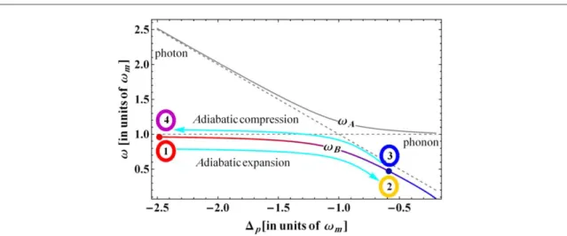
References[7–9] describe a quantum heat engine which makes use of polariton excitations in an optomechanical system(without feedback) as working fluid. This device requires strong optomechanical coupling and resolved sideband regime wm,Gkcfor its functioning. And works at red detuning, where the laser frequency is lower than the cavity frequency so that the optical and mechanical mode can exchange coherently their excitations. Only in this regime the hybridised polariton excitations(the excitations of the normal modes of the system) become relevant. The engine focuses on the lower polariton mode and realises an Otto cycle formed by two adiabatic and two isochoric processes. Specifically it works as follows (see figure2). The lower polariton
frequency plays the role of the volume of the workingfluid (similar to other single oscillator engines [1,2]) and it can be controlled via the laser detuning. This is the central tool used to operate the engine through the four strokes of the cycle. At large detuning the lower polariton is phonon-like and it is in thermal contact with the hot
mechanical thermal bath(see figure2). A fast change of the detuning brings the laser closer to the cavity resonance, passing through the red mechanical sideband, until the polariton becomes photon-like and comes into contact with the cold(zero temperature) optical bath. This variation of the detuning realizes the first adiabatic process from 1 to 2(see figure2). Hence it has to be sufficiently fast in order to avoid dissipation. However, at the same time, it has to be sufficiently slow in order to avoid non-adiabatic transitions to the upper polariton mode. This means that the durationτ1of this process must fulfil the conditions1 Gt11 kc (note that the linearized optomechanical coupling is assumed constant during the cycle; this can be achieved by properly controlling the pump intensity during the adiabatic processes[7–9]). After the adiabatic process, the detuning is keptfixed at the value closest to the cavity resonance for a time τ2?1/κcuntil the lower (photon-like) polariton thermalizes with the optical reservoir realising the first isochoric process. This process has to be sufficiently short (τ2=1/γ) in order to avoid mechanical dissipation of the upper(phonon-like) polariton which should not contribute to the variation of the system energy during the cycle. The second adiabatic process is realized by sweeping back the detuning to the initial value over a timeτ3=τ1so to guarantee the adiabaticity of the process. Now, the lower polariton is again phonon-like and in the second isochoric process it thermalizes with the thermal mechanical bath, over a timeτ4?1/γ. The upper polariton, instead, does not change significantly its number of excitations during the full cycle.
4. The feedback-enabled heat engine
A critical requirement in this device is the ability to realise the adiabatic processes which needs a sufficiently large difference between G andκc. This is the regime of strong coupling that, although reached in a few systems [22,23], is not straightforward to achieve, and in certain cases it is inhibited by the onset of detrimental nonlinear effects[16]. As discussed in [16], the feedback that we have described above seems particularly fit for this purpose, and can be exploited to ease the realisation of this engine. In particular, on the one hand the feedback loop enables one to reduce the cavity bandwidth and to bring a system into the strong coupling regime even if naturally it is weakly coupled; on the other hand it adds extra noise to the cavity, corresponding to afinite number of thermal photonic excitations nopt,fb. In order to realize the heat engine that works on the lower polariton, the cycle should work between a cold photonic reservoir and a hot phononic reservior. This means that the Otto cycle that we have discussed can be effective as long asnopt,fb<nth, which implies(see
equation(14)) that κfbcannot be too small. Furthermore, a difference between the model of[7,8] and the feedback-controlled system introduced in section2is the additional parametric driving in the latter(see equation(9)). However when the system is in the resolved sideband regime its effect is very small. Hence, neglecting the parametric term we can perform an analysis similar to the one discussed above also in the case of feedback. And we can state that, when one utilises feedback, the engine can work efficiently when the duration of the four strokes fulfil the following set of relations
Figure 2. Frequency of the two polaritons(upper ωAand lowerωB) of the optomechanical system as a function of the cavity detuning Δpin the red-detuned caseΔp<0 (the optomechanical coupling strength is G=0.05 ωm). The dashed curves correspond to the frequencies of the non-interacting modes. In the plot we have indicated the position of the four nodes of the Otto cycle operated on the lower polariton. The strokes from node 1 to 2 and from 3 to 4 correspond to the adiabatic processes. The strokes from node 2 to 3 and from 4 to 1 take place at constant detuning and correspond to the isochoric processes.
t t k t g t ( ) G 1 , 1 1 , 15 fb 1 3 2 4 and < ( ) nopt,fb n .th 16
If the cycle operates optimally with ideal adiabatic passages, then it realises a perfect Otto cycle where, in the adiabatic processes, the system exchanges energy with the environment in terms of work without transferring heat, instead, in the isochoric processes the system exchanges only heat and thermalizes with the environment (see appendixCfor a definition of heat and work that applies to this system). In this case the heat and the work in each stroke is given by the difference between the system’s energy at the beginning and at the end of each stroke DEij=Ej-Ei(for i, j=1, 2, 3, 4), where, denoting with the label A the upper polariton and with B the lower one, the system energy is given byE=(wANA+wBNB), withωxand Nx(forxÎ {A B, }) the frequency and the number of polariton excitations respectively. The polariton A is initially photon-like and its frequency is given by the initial cavity detuningw ~ DA ∣ i∣, with corresponding number of excitationsNA~nopt,fb. The polariton B, instead, is initially phonon like with frequencyωB∼ωmand NB∼nthexcitations. At the end of the first adiabatic process A becomes phonon-like, at frequency ωA∼ωm, and B photon-like with a frequency close to the corresponding cavity detuning w ~ DB ∣ f∣. Then, in the isochoric process the polariton B thermalizes with the feedback-mediated optical bath, while A should remain with its initial number of excitations. Then, in the second adiabatic process the polariton frequencies return to their initial values, andfinally in the second
isochoric process, polariton B returns to its initial value of excitations(note that during an ideal cycle the number of excitations of the polariton A should remain constant). Hence ideally the changes of energy (and the
corresponding heat Q and work W) in the four strokes, are
w w w w w w = D ~ D + - + D < = D ~ D - D < = D ~ + D - D + > = D ~ - > (∣ ∣ ) ( ∣ ∣ ) ∣ ∣ ∣ ∣ ( ∣ ∣ ) (∣ ∣ ) ( ) W E n n n n Q E n n W E n n n n Q E n n 0, 0, 0, 0. 17 f m m i f f m i f m m m 1 2 1 2 th opt,fb th opt,fb 2 3 2 3 opt,fb th
3 4 3 4 opt,fb opt,fb opt,fb opt,fb
4 1 4 1 th opt,fb
The negative work in thefirst stroke indicates that the work is performed by the system, while the positive heat in the fourth stroke indicates that the heat is absorbed by the system. The efficiency of the cycle is given by the ratio η=−Wtot/Qabsbetween the total workWtot=W12+W34and the absorbed heatQabs=Q41, that is,
h w = - + ~ - D ( ) ∣ ∣ ( ) W W Q 1 . 18 f m 1 2 3 4 4 1
Note that during the adiabatic processes part of the work is also done by and on the polariton A(respectively in thefirst and second adiabatic process). However, since the number of excitations does not change the net contribution to the total work due to polariton A is zero.
4.1. Results
A more accurate estimate of the efficiency and of the work performed by this engine can be computed by focusing on the steady state properties of the lower polariton B alone at the end of each stroke, but still assuming perfect adiabatic processes and constant population of the upper polariton throughout the whole cycle. This allows to better estimate the expected performance of the engine by taking into account also the effects of the optomechanical interaction at large and small detuning. Specifically, equations (2) and (9) can be used to evaluate the steady state correlation matrix ssof the system(see appendixAfor details); moreover, the populations and the frequencies of the polariton mode B can be estimated by transforming the correlation matrix to the polariton bases, which determines the normal modes of the system Hamiltonian as discussed in appendixB. This allows to estimate the energy associated to the polariton B at the beginning and end of each stroke(EB j, =wB j, NB j, for j=1, 2, 3, 4) and to estimate the corresponding work and heat (such as
~ -( - + - )
Wtot EB,2 EB,1 EB,4 EB,3 andQabs~EB,1-EB,4). The corresponding results are reported in figure3. They show that the optimal performance of the engine are achieved at smallΔpand G[7,8]. In this regime however our estimate are likely to be inaccurate. In fact, on the one hand, at vanishing G the time for the adiabatic passage needs to be extremely long(longer then the dissipation time), and on the other hand at small Δpthe effect of the parametric term can become important(in fact at very small Δfthe system is unstable(see appendixC) as indicated by the white areas in figure3). In order to address this issue more rigorously we have analysed the full dynamics of the system.
An in-depth study of the efficiency of the engine is achieved by solving the quantum Langevin equations (2) and(9), and computing the time evolution of the energy exchanged between the system and the environment in terms of heat and work as discussed in appendixC. Specifically, these quantities can be expressed in terms of the correlation functions of the system operators, the dynamics of which can be computed by standard techniques
(see appendixA). Hereafter we report and discuss the result of this numerical analysis when the cavity detuning Δpis changed in time, in order to realise the Otto cycle, according to the relation
D = - + D < D < - + D < D D - D -D - -D -⎧ ⎨ ⎪ ⎪⎪ ⎩ ⎪ ⎪⎪ ( ) ( ) ( ) ( ) t t t t t t t t t t t t t t t t t , , , , . 19 p t t i f t t f i 0 0 1 1 2 2 2 2 3 4 f i i f 1 0 3 2
In details(see figure4), in the first stroke the detuning is changed linearly from the initial value ΔitoΔf. Then it is kept constant at the valueΔf. In the third stroke it changes linearly back to the initial value. Andfinally, in the last stroke, it remains constant at the valueΔi. The duration of each stroke is t =j t1-tj-1, for j=1, 2, 3, 4.
Infigure5we report the results evaluated for an optomechanical coupling G of the same order of the cavity decay rateκc. In this case the engine described in[7,8] has low efficiency. Here we utilize feedback to effectively reduce the cavity linewidth and reach the regime of strong coupling[16] and significantly enhance the
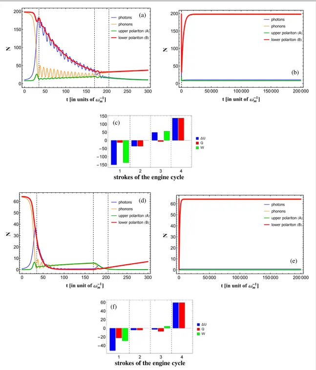
performance of the engine. Figure5(a) shows that the lowest polariton B plays the main role in the dynamics of the system, and we can ignore the dynamics of the polariton A as the variation of its excitations is relatively small during each stroke of the Otto cycle. At the beginning of the process, the number of excitations of the upper and lower polariton modes, NAand NB, are almost equal to the number of photons Naand phonon Nbrespectively.
Figure 3.(a) Thermal efficiency η and (b) total work Wtotdone by the engine(operated on the lower polariton) as a function of the smallest detuningΔfand the optomechanical coupling strength G, evaluated in terms of the steady-state energy corresponding to the lower polariton mode at each node of cycle, assuming perfect adiabatic processes and constant excitations of the upper polariton mode. The white areas indicate the parameter regime at which the system is unstable(see appendixC). The dots indicate the parameters used for the results infigures5and6. The other parameters areΔi=−3ωm, 2κc=0.1ωm,2g=10-4wm, and nth=300. The feedback is set in order to achieve the effective cavity decay rate 2κfb=0.015ωm, corresponding to an effective number of thermal photonsnopt,fb»8(see equation (14)).
Figure 4. Time evolution of the detuningΔp. The vertical dashed lines indicate the end and the beginning of each stroke. The last stroke is not shown completely because it is very slow due to the small mechanical damping rateγ. During the last stroke the Δp remains constant.
The numbers of polaritons NAand NBremain almost constant during thefirst adiabatic passage (while at the same time the phonon and photon numbers exchange their values). In the second stroke the photon-like B-polaritons decay due to cavity dissipation(the oscillations of the photon and phonon populations are due to the optomechanical coupling). In the third stroke the polariton mode B comes back to its phonon-like character, and then it slowly thermalizes to its initial population. Thefinal thermalization is shown in plots (b) and (e) because it is very slow due to the small mechanical damping rateγ. This behaviour is consistent with that of an Otto cycle as discussed in section4[7,8]. It is also worth to notice that the population of polariton A remains small throughout the whole cycle, indicating that it plays a minor role in the energy exchanges and hence in the functioning of the engine. Figure5(c) shows the changes in energy, work and heat in each stroke. As expected for an Otto cycle, thefirst and third strokes (the adiabatic passages) are mainly associated with work production, while heat is exchanged mainly in the isochoric processes(second and fourth strokes). In particular, the system
Figure 5.(a), (b), (d), (f) Time evolution of the populations of the polariton modes, NB(red line) and NA(green line), and of the photonic(Na, blue line) and phononic modes (Nb, orange line) during a loop of the engine cycle (with initial state given by the system steady state at the initial detuning) with (a), (b) and without (d), (e) feedback. (a) and (d) show the dynamics in the first three strokes. (b) and (d) show a longer time scale that highlight the slow thermalization in the fourth stroke. Corresponding energy change (blue), heat exchanged(red) and work performed (green) during each stroke of the cycle. The duration of each stroke is t1=t3=35w-m1,
t =135w
-m
produces work in thefirst stroke, while it absorbs heat in the fourth stroke. The marginal imperfections of figure5(c) (finite heat exchanges in the first and third stroke) are due to non-ideal adiabatic processes [20]. As a comparison we plot infigures5(d)–(f) the corresponding results achievable with the same system when the feedback is off. In this case the cavity dissipation is too large and the population of the polariton mode B
decreases significantly in the first stroke, the work performed is strongly reduced and the corresponding thermal efficiency is much lower.
It is instructive to analyse the performance of the engine in terms of its efficiency, performed work and absorbed heat as a function of the two most critical time scales of the engine dynamics, namely the effective decay rateκfband the duration of the adiabatic processest1 (=t3). These results are shown infigure6. The contour plots highlight that although maximum efficiency and maximum work are not achieved for the same parameters (see the dots in the contour plots), the corresponding values are relatively stable and the results achieved when η is maximum are very close to those corresponding to maximum -Wtot. The work is maximized at intermediate values of bothκfbandτ1, as a compromise between the opposite requirements described by the hierarchy relations(15). The white areas in the contour plots indicate the parameters in which the engine is not functional. Namely for these parameters the total work become positive(indicating that the work is done on the system and not by the system). Plots (b), (c), (e), (f), (h) and (i) represent the values of η, Wtotand Qabs, along the vertical and horizontal lines depicted in the contour plots. The red lines in the plots(b), (e) and (h) correspond to the approximate results evaluated following the procedure used also for the results reported infigure3. We observe that the exact result approaches the estimates close to the optimal values.
Figure 6.(a)–(c): Efficiency of the quantum engine; (d)–(f): total work; (g)–(i): absorbed heat during the cycle, versus κfbandτ1(=τ3), evaluated by computing the system time evolution as discussed in appendixC. The plots in the second column report the values of efficiency (b), work (e) and heat (h) as a function of κfb, for the value ofτ1(=τ3) indicated by the vertical lines in the corresponding contour plots. The green and blue lines correspond to the values that maximize efficiency and work respectively. The red lines correspond to the quantities calculated considering stationary states as infigure3. The plot in the third column report the values of efficiency (c), work (f) and heat (i) as a function of τ1(=τ3), for the value of κfbindicated by the horizontal lines in the corresponding contour plots. The other parameters are the same as those used infigure5.
The work done by this engine can be easily increased by using an higher temperature phonon reservoir. This is shown infigure7, where the number of thermal excitations is increased with respect to the situation of figure3. In these results we have also considered a larger value of the initial detuning, which implies a longer time of the adiabatic processes, and in turn requires a smaller value of the cavity decay rate. The corresponding time evolution of the populations of the system modes is shown infigure7(c) and describes the expected behaviour discussed in section3. Figure8instead displays the corresponding results as a function of the effective cavity decay rateκfband of the duration of the adiabatic processes andt1(=t3)evaluated by solving the dynamics of the full model. We observe that while the efficiency of the engine is only slightly larger than the one achieved with the parameters offigure5, the work done by the system is significantly larger, and it achieves its optimal value when bothκfbandτ1fulfil the relations(15).
Figure3and7show that the optimal performance of the engine is expected for small optomechanical coupling G and smallfinal detuning Δf, and this is confirmed by the results reported in figures9and10. For the parameters used infigure9the system follows more closely the ideal transformations described in section3. Specifically figure9(c) shows the time evolution of the populations of the system modes, with an almost perfect exchange of excitations between cavity and mechanical resonator in thefirst stroke and with NAwhich remains
Figure 7.(a) Thermal efficiency η and (b) total work Wtotdone by the engine as infigure3but with g2 =10-7wm, and nth=5000, Δi=−10ωm, k2 fb= ´2 10-3wm(nopt,fb»80). (c) the time evolution of the population of the polariton and bare modes for the parameters corresponding to the dot in plot(a) and (b) and with t1=t3=500w-m1,τ2=3/κfbandτ4=20/γ.
Figure 8.(a)–(c): Efficiency of the quantum engine; (d)–(f): total work versus κfbandτ1(=τ3), evaluated by computing the system time evolution as discussed in appendixC. The plot in the second column report the values of efficiency (b) and work (e) as functions ofκfb, for the value ofτ1(=τ3) indicated by the vertical lines in the contour plots. The red lines correspond to the quantities calculated considering stationary states as infigure7. The plot in the third column report the values of efficiency (c) and work (f) as a function of τ1(=τ3), for the value of κfbindicated by the horizontal lines in the contour plots. The other parameters are the same as those corresponding tofigure7(c).
essentially constant. Figure10shows that both the efficiency and the work done by the engine are significantly enhanced even if the system(without feedback) is not strongly coupled.
5. The Otto cycle on the upper polariton
In the previous section we have studied the thermodynamical properties of an Otto cycle operated on the lower polariton B. A similar device can be implemented also using the upper polariton A if the following conditions are fulfilled t t g t k t ( ) G 1 , 1 1 , 20 fb 1 3 2 4 > ( ) nopt,fb n ,th 21
such that the cavity effectively decay over the longest time scale and is coupled to the hot bath, meaning that the roles of the hot and cold bath are now exchanged. These conditions can be, in principle, realized with the help of feedback in a system with not to small mechanical dissipation rateγ and low thermal fluctuations. The four strokes of the cycle are then similar to what we have discussed above, and can be realized with a similar variation of the detuning(19), but with the roles of photonic and phononic excitations exchanged (see figure11). Similar to our previous discussion, in this case, we can estimate an engine efficiency of h~ -1 wm ∣Df∣. An example of the performance of this engine is reported infigure12. The results reported infigures12(a) and (b) are
estimates evaluated in terms of the steady state energy of the upper polariton mode at each node of the stroke (assuming the population of the lower polariton mode constant). The efficiency in plot (a) is almost constant as a function of thefinal detuning Δfand this is due to the fact that the frequency of the upper polariton mode is almost constant for values of the detuning close to the cavity resonance(see figure11). The plots in figures12(c) and(d) are the time evolution of the modes populations and the heat and work corresponding to each stroke of the cycle for the parameters indicated by the dot in plots(a) and (b), and computed using the formulas presented in appendixC. They are qualitatively similar to the results offigures5(a) and (c) and demonstrate that for the
Figure 11. Scheme of the Otto cycle operated on the upper polariton(see figure2for the cycle operated on the lower polariton).
Figure 12.(a) Thermal efficiency η and (b) total work Wtotdone by the engine(operated on the upper polariton) as a function of the DetuningΔfand the optomechanical coupling strength G, evaluated in terms of the steady-state quantities corresponding to the upper polariton at each node of the cycle, and assuming perfect adiabatic processes. The white ares indicate the parameters at which the system is unstable(see appendixC). The dots indicate the parameters used for the results in plots (c) and (d). (c) Shows the time evolution of the populations of the polariton and bare modes.(d) Shows the corresponding energy changes (blue), heat exchanged (red) and work performed (green) during each stroke of the cycle. The duration of each stroke is t=t =35w
-m
1 3 1,t2=135w-m1and
t4= 20 kfb. The other parameters areΔi=−3ωm, 2κc=0.1ωm, 2γ=0.012 ωm, and nth=300. The feedback is set in order to achieve the effective cavity decay rate k2 fb= ´2 10-4wmand the effective number of thermal photons nopt,fb≈830.
the corresponding low natural mechanical decay rate, which is by far the lowest rate in the system dynamics, make them very versatile systems which are potential candidates for the experimental investigation of quantum thermodynamical effects. However, in spite of the many proposal of optomechanical based heat engine no experiment has demonstrated such devices so far. It is therefore important to suggest strategies for the
realization of a working optomechanical quantum engine. Here we have shown that the experimental realization of the polariton-based quantum heat engine proposed in[7–9] can be significantly eased by means of a feedback system[16–19] which allows to control the decay rate of the optical cavity. This engine exploits the lower polariton mode as workingfluid and works between the hot phononic thermal reservoir and the cold photonic reservoir with which the polariton comes into contact as the cavity pump detuning is varied around the red mechanical sideband frequency. A critical requirement in this device is the strong coupling regime, that corresponds to an optomechanical interaction strength larger then the cavity decay rate so that the polariton modes can be resolved. In general the coupling strength can be controlled by tuning the driving light power. While, in principle, this could allow to achieve the strong coupling regime, in practice it is often not possible to employ the needed power due to the onset of unwanted nonlinear effects. This is where the feedback realized in [16] can be helpful.
In this work, we have reported a detailed analysis of the performance of the engine when the feedback is employed to effectively reduce the cavity decay rates by driving the system close to the feedback instability threshold. We have demonstrated that the engine can work efficiently even if the system without feedback is not strongly coupled(such that in absence of feedback the polariton modes are not resolved). We have also shown that the feebdack noise, which can be seen as an effective non-zero temperature photonic bath, can be employed to define a similar engine working on the upper polariton mode where the role of the hot and cold baths are exchanged such that the feedback noise is absorbed as heat and transformed into usable work.
The feedback strategy that we have analysed seems easily applicable in any optomechanical system since it requires optical equipment already in use in most of optomechanical experiments. The results that we have presented correspond to systems in the resolved sideband regime and in cryogenic environments(considering a 1 MHz resonator the results infigures3,5,6and12would correspond to an external temperature of 100 mK, the results offigures7–10, instead, would correspond to 1.7 K). Many experimental setups, both in the optical or microwave regimes, can be employed for demonstrating our proposal as for example[22–27]. In order to test the efficiency of this device one should be able to measure the energy variations and to distinguish the contributions due to heat and work. This can be done by measuring the correlation matrix of the system by following for example the approach realized in[24].
To conclude, we highlight that although we have not discussed specific quantum effects, the system that we have studied can be used to study such phenomena. An important example is the investigation of the effects of correlations in the reservoirs which have been predicted to enhance the efficiency of a quantum heat engine beyond the Carnot limit[28]. This could be in principle analysed with our optomechanical system by using, for example, a squeezedfield to drive the cavity [26,29]. Even more interestingly, in our case the bath correlations could be provided by the feedback loop itself[19]. Another related and important question is whether,
correlations in the workingfluid as well could be employed to enhance the efficiency of the engine as discussed in [30]. In our system, in fact, the feedback induced parametric term, which is negligible in the parameter regime that we have considered, could produce additional quantum coherence in the polariton state which may play a relevant role in certain situations. Finally, it is also interesting to ponder if, in some parameter regime, the behaviour of our engine could be interpreted as an instance of a Maxwell’s demon [31] which, in fact, can be seen as a feedback system.
Acknowledgments
We acknowledge the support of the European Union Horizon 2020 Programme for Research and Innovation through the Project No. 732894(FET Proactive HOT) and the Project QuaSeRT funded by the QuantERA ERA-NET Cofund in Quantum Technologies.
Appendix A. The model in matrix form and the correlation matrix
The quantum Langevin equations(2) and (9) can be rewritten in matrix form, in terms of the vector of operators aˆT =( ˆ ˆ ˆa b a, , †,bˆ )†, as
= +
ˆ˙ ˆ ˆ ( )
a a Q a ,in A.1
where the drift matrix is
k k k g w k k k g w = -- D -+ - - + D -- - -⎛ ⎝ ⎜ ⎜ ⎜ ⎜ ⎞ ⎠ ⎟ ⎟ ⎟ ⎟ ( ) G G G G G G G G i i i i i i 0 i i i i 0 i i , A.2 p c m c p m fb fb fb fb
the matrixis given by
k g k g = ⎛ ⎝ ⎜ ⎜ ⎜ ⎜ ⎜ ⎞ ⎠ ⎟ ⎟ ⎟ ⎟ ⎟ ( ) Q 2 0 0 0 0 2 0 0 0 0 2 0 0 0 0 2 , A.3 fb fb
and ˆainis the vector of noise operator aˆ =( ˆa ,bˆ ,aˆ†,bˆ )†
inT in in in in. From equation(A.1) one finds that the evolution of the correlation matrix
= á ñ = á ñ á ñ á ñ á ñ á ñ á ñ á ñ á ñ á ñ á ñ á ñ á ñ á ñ á ñ á ñ á ñ ⎛ ⎝ ⎜ ⎜ ⎜ ⎜ ⎜⎜ ⎞ ⎠ ⎟ ⎟ ⎟ ⎟ ⎟⎟ ˆ ˆ ˆ ˆ ˆ ˆ ˆ ˆ ˆ ˆ ˆ ˆ ˆ ˆ ˆ ˆ ˆ ˆ ˆ ˆ ˆ ˆ ˆ ˆ ˆ ˆ ˆ ˆ ˆ ˆ ˆ ˆ ˆ ˆ ( ) † † † † † † † † † † † † † † † † a a aa ab aa ab ba bb ba bb a a a b a a a b b a b b b a b b , A.4 T is given by ˙ =+T +Q Q, (A.5) in where inis the correlation matrix of the noise operators
= á ñ = + + ⎛ ⎝ ⎜ ⎜ ⎜⎜ ⎞ ⎠ ⎟ ⎟ ⎟⎟ ˆ ˆ ( ) a a n n n n 0 0 1 0 0 0 0 1 0 0 0 0 0 0 A.6 T in in in opt,fb th opt,fb th
(note that in the absence of the feedback we have κfb=κcandnopt,fb=0).
By defining = QinQand introducing the linear super operatorˆso that ˆ C=C+CTwe can find the stationary correlation matrix
= - ˆ- . (A.7)
ss
1
Appendix B. Polariton description of the system
The Hamiltonian corresponding to the quantum Langevin equations(2) and (9) is
w k k = - D + + + + - - -ˆ ˆ ˆ† ˆ ˆ† ( ˆ ˆ )( ˆ† ˆ )† ( ˆ ˆ )† ( ) H a a b b G b b a a i a a 2 . B.1 p m c fb fb 2 2
The uncoupled normal modes of ˆHfb, i.e. the polariton modes, can be expressed in terms of the bare operators ˆ
a(aˆ†) andbˆ(ˆ†
w k k w = -D -⎝ ⎜ ⎜ ⎜ ⎠ ⎟ ⎟ ⎟ ( ) ( ) G G G G G G 2 0 i 0 , B.5 m p c m fb
and the diagonal matrix of symplectic eigenvalues, defined as = 12 diag{w wA, B,-wA,-wB}where
w = 1 D - (k -k ) +w + [D -(k -k ) -w ] - G D w ( ) 2 16 , B.6 A 2p c fb 2 m2 p2 c fb 2 m2 2 2 p m w = 1 D -(k -k ) +w - [D -(k -k ) -w ] - G D w ( ) 2 16 . B.7 B 2p c fb 2 m2 2p c fb 2 m2 2 2 p m
Infigure2, we have depicted these eigenfrequencies in the red detuning regime(Δp<0) where the beam-splitter interaction term of the Hamiltonian of equation(B.1) plays the dominant role [7]. The Hamilto-nian(B.1) is stable, and the polariton modes can be defined, whenever the lowest eigenfrequency ωBis real positive, i.e. when D < - Gp 2 2/wm- 4G4 wm2 +(kc-kfb)2.
The correlation matrixpfor the polariton modes
= á ñ = á ñ á ñ á ñ á ñ á ñ á ñ á ñ á ñ á ñ á ñ á ñ á ñ á ñ á ñ á ñ á ñ ⎛ ⎝ ⎜ ⎜ ⎜ ⎜ ⎜ ⎞ ⎠ ⎟ ⎟ ⎟ ⎟ ⎟ ˆ ˆ ˆ ˆ ˆ ˆ ˆ ˆ ˆ ˆ ˆ ˆ ˆ ˆ ˆ ˆ ˆ ˆ ˆ ˆ ˆ ˆ ˆ ˆ ˆ ˆ ˆ ˆ ˆ ˆ ˆ ˆ ˆ ˆ ( ) † † † † † † † † † † † † † † † † A A AA AB AA AB BA BB BA BB A A A B A A A B B A B B B A B B , B.8 p T
is related to the bare modes correlation matrix by the relation
= - ( -) . (B.9)
p 1 1T
In particular the steady state in the polariton base is obtained by computing equation(B.9) on the steady state correlation matrix(A.7). The steady state population of the polariton B is then given by the element (4, 2) of the resulting matrix(see (B.8)), i.e.NB= { }p 4,2, and similarlyNA= { }p 3,1.
Appendix C. Heat and work
The internal energy U of the system can be expressed in terms of the average of the system Hamiltonian[1] r
= á ñ =
( ) ˆ ( ) [ ˆ ( ) ˆ ( )] ( )
U t Hfb t Tr t Hfb t C.1
whereρ(t) is the density matrix which describes the state of the system at time t, and Hfb(t) is the system Hamiltonian(B.1), with time dependent detuning Δp(t). The energy change is given by the temporal derivative of the internal energy
r r
= +
˙ ( ) [ ˆ ( ) ˆ˙ ( )] [ ˆ˙ ( ) ˆ ( )] ( )
U t Tr t H t Tr t H t , C.2
which is the sum of two contributions. Thefirst, associated with the variation of the system Hamiltonian, contributes to the work, while the second one is due to irreversible dissipative processes and contributes to the heat[32]. Specifically, in a process that takes place from the initial time tito thefinal time tf, the heat Q and the work W are defined by the time integrals
ò
r = [ ˆ˙ ( ) ˆ ( )] ( ) Q d Trt t H t , C.3 t t fb i fò
r = [ ˆ ( ) ˆ ( )] ( ) W d Trt t H t , C.4 t t fb i f such that + = D ( ) Q W U C.5which represent thefirst law of thermodynamics. The difference in internal energy DU can be computed in terms of the average values of the system Hamiltonian(B.1), as D = áU H tfb( )f ñ - áH tfb( )iñ. In particular, the average valueáH tfb( )ñcan be expressed in terms of the second order correlation functions(which in turn are
derived using the solution of the equation for the correlation matrix(A.5) evaluated using the time dependent detuning(19)) as w k k á ñ = - D á ñ + á ñ + á ñ + á ñ + á ñ + á ñ - - á ñ - á ñ ˆ ( ) ( ) ˆ ( ) ˆ ( ) ˆ ( ) ˆ( ) [ ˆ ( ) ˆ ( ) ˆ ( ) ˆ ( ) ˆ ( ) ˆ( ) ˆ ( ) ˆ ( ) ] [ ˆ ( ) ˆ ( ) ] ( ) † † † † † † † H t t a t a t b t b t G b t a t b t a t b t a t b t a t a t a t i 2 . C.6 p m c fb fb 2 2
The heat, instead, can be computed by substituting the system Hamiltonian(B.1) and the system master equations r r k r r r k r r r g r r r g r r r = - + + - - + - -+ + - - + - -ˆ [ ˆ ( ) ˆ ] ( )( ˆ ˆ ˆ ˆ ˆ ˆ ˆ ˆ ˆ) ( ˆ ˆ ˆ ˆ ˆ ˆ ˆ ˆ ˆ ) ( )( ˆ ˆ ˆ ˆ ˆ ˆ ˆ ˆ ˆ) ( ˆ ˆ ˆ ˆ ˆ ˆ ˆ ˆ ˆ ) ( ) † † † † † † † † † † † † H t n a a a a a a n a a aa aa n b b b b b b n b b bb bb i , 1 2 2 1 2 2 C.7 c c fb opt,fb opt,fb th th
(which provides a description of the system dynamics equivalent to the quantum Langevin equations (2) and (9)), into equation (C.3). Thereby, exploiting the cyclic property of the trace, one finds that the heat exchanged with the environment in a process from time tito tfis given by
ò
rò
w g k k w gk k g k k k = = - D + D á ñ - á ñ - + á ñ + á ñ + á ñ + á ñ + - á ñ - á ñ [ ˆ ( ) ˆ ( )] { ( ) ( ) ˆ ( ) ( )ˆ ˆ ( ) ˆ( ) ( )[ ˆ ( ) ˆ ( ) ˆ ( ) ˆ ( ) ˆ ( ) ˆ( ) ˆ ( ) ˆ ( ) ] ( )[ ˆ ( ) ˆ ( ) ]} ( ) † † † † † † † Q t t H t t n t n t a t a t b t b t G b t a t b t a t b t a t b t a t a t a t d Tr d 2 2 2 2 i . C.8 t t t t m p c p c m c c c c fb th opt fb 2 2 i f i fThe correlation functions in this expression can be computed by solving the equation for the correlation matrix(A.5) (with the time dependent detuning). Finally, the work is determined, in terms of these results for ΔU and Q, using the first law of thermodynamics(C.5).
We notice that this approach allows to extend the numerical analysis introduced in[7–9] (which, being based on the numerical integration of the master equation, is constrained to a low number of system excitations) to an arbitrary number of excitations.
References
[1] Vinjanampathy S and Anders J 2016 Quantum thermodynamics Contemp. Phys.57 545–79
[2] Alicki R and Kosloff R 2018 Introduction to quantum thermodynamics: history and prospects arXiv:1801.08314[quant-ph] [3] Bowen W P and Milburn G J 2015 Quantum Optomechanics (London: Taylor and Francis)
[4] Li B-B, Bílek J, Hoff U B, Madsen L S, Forstner S, Prakash V, Schäfermeier C, Gehring T, Bowen W P and Andersen U L 2018 Quantum enhanced optomechanical magnetometry Optica5 850
[5] Aspelmeyer M, Kippenberg T J and Marquardt F 2014 Cavity optomechanics Rev. Mod. Phys.86 1391–452 [6] Bawaj M et al 2015 Probing deformed commutators with macroscopic harmonic oscillators Nat. Commun.6 7503 [7] Zhang K, Bariani F and Meystre P 2014 Quantum optomechanical heat engine Phys. Rev. Lett.112 150602 [8] Zhang K, Bariani F and Meystre P 2014 Theory of an optomechanical quantum heat engine Phys. Rev. A90 023819
[9] Dong Y, Zhang K, Bariani F and Meystre P 2015 Work measurement in an optomechanical quantum heat engine Phys. Rev. A92 033854
[10] Dong Y, Bariani F and Meystre P 2015 Phonon cooling by an optomechanical heat pump Phys. Rev. Lett.115 223602 [11] Dechant A, Kiesel N and Lutz E 2015 All-optical nanomechanical heat engine Phys. Rev. Lett.114 183602
[12] Mari A, Farace A and Giovannetti V 2015 Quantum optomechanical piston engines powered by heat J. Phys. B: At. Mol. Opt. Phys.48 175501
[13] Gelbwaser-Klimovsky D and Kurizki G 2015 Work extraction from heat-powered quantized optomechanical setups Sci. Rep.5 07809 [14] Bathaee M and Bahrampour A R 2016 Optimal control of the power adiabatic stroke of an optomechanical heat engine Phys. Rev. E94
022141
[15] Zhang K and Zhang W 2017 Quantum optomechanical straight-twin engine Phys. Rev. A95 053870
[16] Rossi M, Kralj N, Zippilli S, Natali R, Borrielli A, Pandraud G, Serra E, Di Giuseppe G and Vitali D 2018 Normal-mode splitting in a weakly coupled optomechanical system Phys. Rev. Lett.120 073601
[17] Rossi M, Kralj N, Zippilli S, Natali R, Borrielli A, Pandraud G, Serra E, Di Giuseppe G and Vitali D 2017 Enhancing sideband cooling by feedback-controlled light Phys. Rev. Lett.119 123603
[26] Clark J B, Lecocq F, Simmonds R W, Aumentado J and Teufel J D 2017 Sideband cooling beyond the quantum backaction limit with squeezed light Nature541 191–5
[27] Shomroni I, Qiu L, Malz D, Nunnenkamp A and Kippenberg T J 2019 Optical backaction-evading measurement of a mechanical oscillator Nat. Commun.10 2086
[28] Niedenzu W, Mukherjee V, Ghosh A, Kofman A G and Kurizki G 2018 Quantum engine efficiency bound beyond the second law of thermodynamics Nat. Commun.9 165
[29] Asjad M, Zippilli S and Vitali D 2016 Suppression of Stokes scattering and improved optomechanical cooling with squeezed light Phys. Rev. A94 051801
[30] Klatzow J, Becker J N, Ledingham P M, Weinzetl C, Kaczmarek K T, Saunders D J, Nunn J, Walmsley I A, Uzdin R and Poem E 2019 Experimental demonstration of quantum effects in the operation of microscopic heat engines Phys. Rev. Lett.122 110601 [31] Lloyd S 1997 Quantum-mechanical Maxwellʼs demon Phys. Rev. A56 3374–82
![Figure 1. The feedback loop: a quadrature of the field, transmitted through a Fabry–Pérot cavity with a movable end mirror, is detected via homodyne detection at phase θ fb , and the corresponding photocurrent is used to modulate the input field [ 19 ].](https://thumb-eu.123doks.com/thumbv2/123dokorg/5397689.57697/3.892.173.829.93.343/feedback-quadrature-transmitted-detected-detection-corresponding-photocurrent-modulate.webp)