Local Propagation in Neural Network Learning by Architectural Constraints

Dipartimento di Ingegneria dell’Informazione e Scienze Matematiche

DI

Local Propagation in Neural Network

Learning by Architectural Constraints

Matteo Tiezzi

Ph.D Thesis in Information Engineering and Science

Supervisor Prof. Marco Maggini

A crucial role for the success of the Artificial Neural Networks (ANN) pro-cessing scheme has been played by the feed-forward propagation of signals. The input patterns undergo a series of stacked parametrized transformations, which foster deep feature extraction and an increasing representational power. Each artificial neural network layer aggregates information from its incoming connections, projects it to another space, and immediately propagates it to the next layer.

Since its introduction in the ’80s, BackPropagation (BP) is considered to be the “de facto” algorithm for training neural nets. The weights associated to the connections between the network layers are updated due to the backward pass, that is a straightforward derivation of the chain rule for the computation of the derivatives in a composition of functions. This computation requires to store all the intermediate values of the process. Moreover, it implies the use of non-local information, since the activity of one neuron has the ability to affect all the subsequent units up to the last output layer.

However, learning in the human brain can be considered a continuous, life-long and gradual process in which neuron activations fire, leveraging local information, both in space, e.g neighboring neurons, and time, e.g. previous states.

Following this principle, this thesis is inspired by the ideas of decoupling the computational scheme, behind the standard processing of ANNs, in order to decompose its overall structure into local components. Such local parts

particular, a set of additional variables are added to the learning problem, in order to store the information on the status of the constrained neural units. Therefore, it is possible to describe the computations performed by the net-work itself guiding the evolution of these auxiliary variables via constraints. This choice allows us to setup an optimization procedure that is “local”, i.e., it does not require (1) to query the whole network, (2) to accomplish the diffusion of the information, or (3) to bufferize data streamed over time in order to be able to compute gradients. The thesis investigates three different learning settings that are instances of the aforementioned scheme: (1) con-straints among layers in feed-forward neural networks, (2) concon-straints among the states of neighboring nodes in Graph Neural Networks, and (3) constraints among predictions over time.

. . . , here we go again. Three years after the last time, keeping the tradition of writing overnight. Maybe because it is the most inspiring moment, the silence broken solely by the typewriting on the keyboard. Nothing seems to have changed, but in reality lots of things have been overthrown, revolutionized.

This last part has been tough. I am not referring uniquely to the writing of this dissertation, but the overall final period. Decisions to be taken, deadlines to be respected, audience to be satisfied. But fortunately, this whole path and the people I have met in the last years have trained me to cope with it and have supported me in all the possible (both physically and, recently, remotely ) ways.

Firstly, this whole experience was possible thanks to my advisor Marco Maggini, to his readiness, the last-hour corrections, his clever comments and his decision to talk to me about that Machine Learning scholarship, almost four years ago, on the fourth floor. It all started in that way, and I was not even remotely imagining how powerful that choice could affect my life. A decision that could not have been possible also without Prof. Trentin, his slides, his ability to impressively teach AI and tell strange stories. I owe to him (and to the lana caprina) my interest in this amazing discipline. Other thanks to Marco Gori, to his warm welcome into our SAILab, his stunning speech ability and the insightful talks, the powerful phone calls. Thanks to the other Prof. of the lab, Michelangelo for his multiple incredible abilities, Monica (thanks indeed.) and especially to Franco Scarselli, his kindness, visionary mind and his attention to details in our discussions on GNNs.

I want to reserve a special thanks to Stefano Melacci, without whom many of the work I have done during these three years would not have been possible. Thanks for being always ready to help, to give me insightful comments, to teach me how a researcher must behave, for the post-calls. I always try to follow the suggestion I received from Achille, learn as much as you can from Stefano. I will try my best.

I surely will remember these years for the challenges, struggles, late night work (nothing

order, to Lisa for always being there from the first day, to Luca for all the discussions and advises, for being a friend, thanks to Alessandro, Sara, Vincenzo, Simone and Paolo for their availability, courtesy, the tales and the laugh, for the whole time spent together. Thanks to Gabriele, for the questions and insightful doubts and for the amazing trip to NY. Thanks to Enrico for being my new code mate, for the memes, for the adversities and bugs we will defeat together in the next years. Furthermore, I am grateful to have met amazing friends as Francesco, always ready to help, to advise me (also songs), to guide me from the first day at the lab; as Dario, for our laughs, his attention to details, for being a charismatic steady point in the lab, for Re Mida and the interview; as Giuseppe, always inspiring for his astonishing extra gear, for all the fruitful discussions, collaborations and fun, for the beautiful experience of his wedding with Maria.

Then I want to thank some old great friends that are travelling with me, since many years, along the strenuous manifold of life. Thanks to Alberto for the many laughs, videos, car travels, nights out, code debugging, for his intuitions and for asking me to work together on GNNs during the first PhD year. Thanks to Marco for always being ready to support me (and I hope to have done the same for him, I always will) even if we are far apart. For always being there for the big decisions. And I want to thank Andrea, an amazing friend, a brilliant researcher, a great roommate. Thanks for the talks, all the messages, the dinners, the laughs and the advises, for all this period. Furthermore, I am not able to express in simple words my appreciation to Giorgia, for being so important to me during this last period. Thanks for the wonderful talks, for the walks and all, for the time spent together. For showing me my weaknesses and for looking after (and to) me. Everyday. Thanks.

Concluding this three years recap, this time I will try not to be too sentimental with my family, hopefully without tear drops. Even if actually all the thanks I can imagine are not enough, given the support, affection (and many other kind words) my parents, my awesome brother and my grandma give me daily (even if I am not always accessible). Thanks for being always with me. Thanks for this wonderful travel.

This PhD experience have brought me many new amazing experiences, discoveries, situations, fun and distress. My main regret is the fact that one of the greatest experiences I had, coincided and made impossible for me to give a proper farewell to an important person of my life. The time just flew away. I will try my best to pursue my path in order to not make that missed greeting worthless.

Ave atque vale.

Siena, December 2020

Abstract . . . i

Acknowledgements . . . iii

1 Introduction 3 1.1 Motivations . . . 6

1.2 Research questions and contributions . . . 8

1.3 Thesis structure . . . 10

1.4 List of Publications . . . 11

2 Neural Network Architecture as Constraints 15 2.1 Artificial Neural Architectures . . . 16

2.1.1 Multi-Layer Perceptrons . . . 16

2.1.2 Recurrent Neural Networks . . . 18

2.1.3 Convolutional Neural Networks . . . 19

2.1.4 Graph Neural Networks . . . 22

2.2 Learning by BackPropagation . . . 25

2.2.1 Learning in Structured Networks . . . 30

2.2.2 Complexity Analysis . . . 31

2.3 Regularization . . . 31

2.4 The Lagrangian formalism . . . 32

2.5 A Lagrangian framework for BackPropagation . . . 34

2.6 Constrained differential optimization . . . 37 v

3 Local Propagation in Neural Networks 41

3.1 Related Work . . . 43

3.2 Constraint-based Neural Networks . . . 44

3.3 Local Propagation in Constraint-based Neural Networks . . . . 46

3.3.1 Properties of Local Learning . . . 47

3.3.2 Epsilon-insensitive Constraints . . . 51

3.4 LP formulation for Neural Models . . . 52

3.5 Experiments . . . 55

3.6 Discussion . . . 60

4 Lagrangian Propagation Graph Neural Networks 63 4.1 Related Work . . . 65

4.1.1 Extending ANNs to graphs . . . 66

4.1.2 The role of aggregation functions . . . 67

4.1.3 Other recent trends . . . 68

4.2 Constraint-based Propagation in Graph Neural Networks . . . . 68

4.2.1 A Local Learning formulation . . . 69

4.2.2 A mixed optimization strategy . . . 71

4.2.3 LP-GNN Complexity analysis . . . 73

4.3 Deep LP-GNNs . . . 73

4.3.1 Deep LP-GNN Complexity analysis . . . 75

4.4 Experiments . . . 75 4.4.1 Qualitative analysis . . . 75 4.4.2 Artificial Tasks . . . 77 4.4.3 Graph Classification . . . 80 4.4.4 Depth vs Diffusion . . . 83 4.5 Discussion . . . 84

5 Feature learning in video streams 87 5.1 Preliminaries and Related Work . . . 89

5.1.1 Lifelong learning over time . . . 89

5.1.2 Unsupervised Learning by Mutual Information Maxi-mization . . . 89

5.1.3 Cognitive Action Laws: Learning Over Time . . . 91

5.2 Introducing Second-Order Laws . . . 96 vi

5.2.1 A Temporally local computational model . . . 98

5.3 Mutual Information in Video Streams . . . 99

5.4 Constraining predictions over-time . . . 101

5.5 Restricting Computations on Salient Areas . . . 103

5.6 Experimental Results . . . 106

5.7 Discussion and Future Work . . . 112

6 Conclusions and Future Works 115 6.1 Summary of Contributions . . . 115

6.2 Issues and future research directions . . . 117

6.2.1 Local Propagation . . . 117

6.2.2 Lagrangian Propagation GNNs . . . 119

6.2.3 Constraining Predictions over time . . . 120

Bibliography 123

1.1 The computational graph definition of Artificial Neural Net-works. . . 5 1.2 BackPropagation on the computational graph of ANNs

exploit-ing the Chain Rule (in red). . . 5 1.3 The decomposition of the computational graph into local

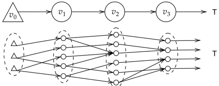
com-ponents, connected via constraints. . . 7 2.1 Instance of the computational graph (top) as a Multi–Layer

Perceptron (bottom). A set of neurons at the same depth – layer – of the data-flow are denoted by the same node vi. To

ease the plot comprehension, we depict an MLP with sparse connections among neurons. . . 17 2.2 The mapping defined by the Sigmoid, Hyperbolic Tangent (Tanh)

and Rectified Linear Unit (ReLU) activation functions. . . 19 2.3 2D convolution of an input tensor I and a kernel K (Figure

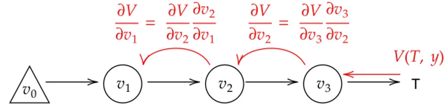
thanks to Petar Veličković). . . 20 2.4 The Graph Neural Network model. . . 26 2.5 BackPropagation on a generic computational graph exploiting

the Chain Rule (in red). . . 27 2.6 In BDMM [1] the state x is attracted toward the constraint

subspace. The state slides along the subspace moving to the minima of the function f(·), undergoing damped oscillations dictated by the differential equations. . . 38

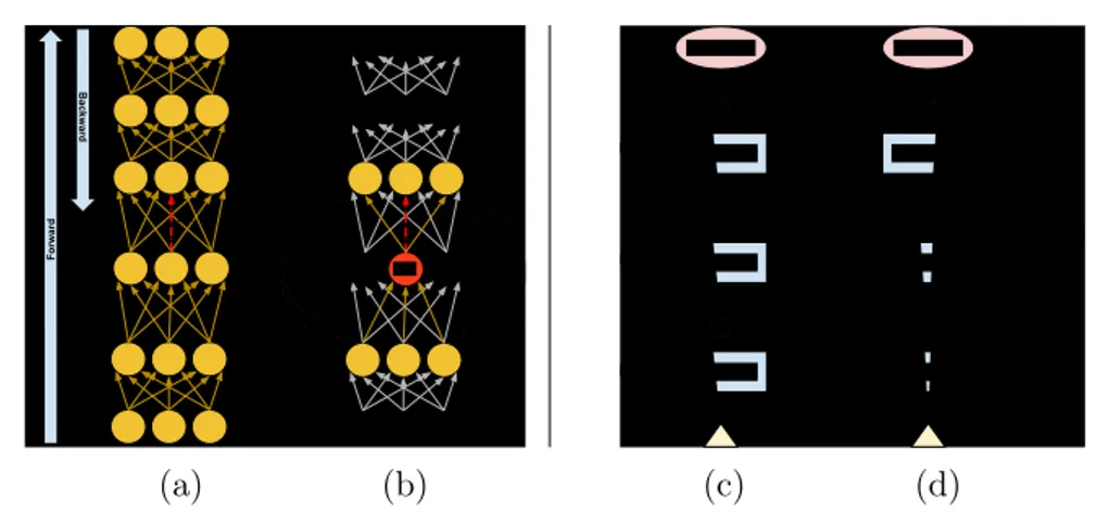
3.1 Left: the neurons and weights that are involved in the com-putations to update the red-dotted weight w are highlighted in yellow. (a) BackPropagation; (b) Local Propagation – the com-putations required to update the variables x, λ (associated to the red neuron) are also considered. Right: (c) ResNet in the case of H = 3, and (d) after the change of variables (xℓ → x˜ℓ)

described in Sec. 3.4. Greenish circles are sums, and the nota-tion inℓ inside a rectangular block indicates the block input. . . 48

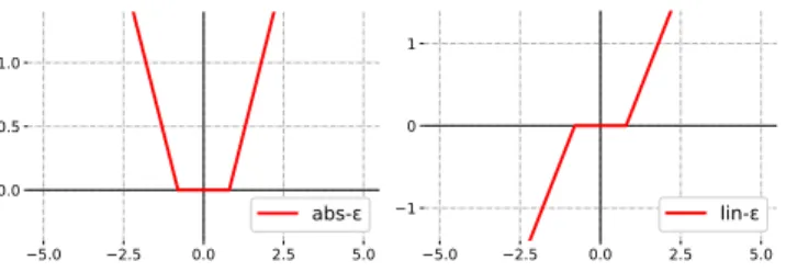
3.2 The mapping defined by the ε-insensitive functions, abs-ε and lin-ε. . . 51 3.3 Accuracies of BP and LP (with different ε-insensitive functions,

abs-ε, lin-ε) on the MNIST data. . . 57 3.4 Convergence speed of BP and LP in the MNIST dataset (left),

and in the Letter data (right). . . 58 4.1 The karate club dataset. This is a simple and well-known

dataset exploited to perform a qualitative analysis of the be-haviour of our model. Nodes have high intra-class connections and low inter-class connections. Each color is associated to a different class (4 classes). . . 76 4.2 Evolution of the node state embeddings at different stages of

the learning process: beginning, after 200 epochs and at conver-gence. We are not exploiting any node-attached features from the available data, so that the plotted node representations are the outcome of the diffusion process only, which is capable of mapping the topology of the graph into meaningful latent rep-resentations. Each node is represented with the color of the given corresponding class (ground truth), while the four back-ground colors are the predictions of the output function learned by our model. The model learns node state embeddings that are linearly separated with respect to the four classes. . . 77 4.3 An example of a subgraph matching problem, where the graph

with the blue nodes is matched against the bigger graph. . . . 78 x

4.4 An example of a graph containing a clique. The blue nodes represent a fully connected subgraph of dimension 4, whereas the red nodes do not belong to the clique. . . 79 5.1 The goal of the learning process is the maximization of the

in-formation transfer (I(X, Y )) from the input visual stream X to the m-dimensional output space Y of a multi-layer convolu-tional network with ℓ layers. . . 100 5.2 On the left, a depiction of the spatial uniform probability

den-sity commonly exploited in image procesing – all the pixels equally contribute to the learning process. On the right side, a human-like focus of attention, denoted with the red cross, filters relevant information in the visual scene. . . 104 5.3 Sample frames taken from the SparseMNIST, Carpark, Call

streams, left-to-right. . . 107 5.4 For each stream, we show (left) the areas mostly covered by

FOA (blue: largest attention), and (right) the scatterplots of the fixation points, with hue denoting the magnitude of the FOA velocity (blue: slower; yellow: faster). Low-speed move-ments happen on the most informative areas (e.g., digits, busy roads, human presence/movement, respectively). . . 108 5.5 Comparison between models trained on a regular trajectory of

the attention and on a random trajectory (suffix -Rnd), for architectures S, D, DL. Each bar is about a different training probability density, and the height of the bar is the test MI index along the regular FOA trajectory. . . 112 5.6 Learning dynamics (model D-FOA, different temporal criteria).

The MI index is shown at different time instants. The index at time t is evaluated along the FOA trajectory in the interval [0, t].112

2.1 Common implementations of the state transition function fa().

The function h() is implemented by a feedforward neural net-work with s outputs, whose input is the concatenation of its arguments. . . 24 3.1 Number of patterns, of input features and of output classes in

the datasets exploited for benchmarking the LP algorithm. . . . 56 3.2 Performances of the same architectures optimized with BP and

LP. Left: H = 1 hidden layer (100 units); right: H = 3 hidden layers (30 units each). Largest average accuracies are in bold. . 57 3.3 Accuracies of LP when using (ε > 0) or not using (ε = 0)

ε-insensitive constraints (top-half ) and when using (α > 0) or not using (α = 0) L1-norm-based regularization on the outputs

of each layer (bottom-half ). We report the cases of the abs-ε and lin-ε functions, and we compare architectures with H = 1 hidden layer (100 units) and H = 3 hidden layers (30 units each). . . 59 4.1 The considered variants of the G function. By introducing

ε-insensitive constraint satisfaction, we can inject a controlled amount (i.e. ε) of tolerance of the constraint satisfaction into the hard-optimization scheme. . . 77

4.2 Accuracies on the artificial datasets, for the proposed model (Lagrangian Propagation GNN - LP-GNN) and the standard GNN model for different settings. . . 79 4.3 Average and standard deviation of the classification accuracy

on the graph classification benchmarks, evaluated on the test set, for different GNN models. The proposed model is denoted as LP-GNN and it is evaluated in two different configurations. LP-GNN-Single exploits only one layer of the diffusion mecha-nism, while LP-GNN-Multi exploits multiple layers as described in Section 4.3. It is interesting to note that, even if LP-GNN-Single exploits only a shallow representation of nodes, it per-forms, on average, on-par with respect to other state-of-the-art models. Finally, the LP-GNN-Multi model performs equally to or better than most of the competitors on most of the benchmarks. 81 4.4 Depth vs Diffusion analysis. Absolute (top rows) and Relative

(bottom rows) test accuracies on the IMDB-B dataset when the number of GNN state layers varies from 1 to 5 (i.e. K ∈ [1, 5]. Here, the Relative accuracy represents the percentage of the current accuracy with respect to the maximum obtained perfor-mances. The state-of-the-art GIN [2] model and our proposed approach are compared. . . 85 5.1 Spatial filtering. Mutual Information (MI) index in three video

streams, considering three neural architectures (S, D, DL). Each column (starting from the third one) is about the results of network trained using an input probability density taken from {UNI, FOA, FOAW}, and tested measuring the MI index in all the three density cases (labeled in column “Test”). . . 109 5.2 Temporal locality. Mutual Information (MI) index in three

video streams, considering three neural architectures (S, D, DL). Each column (starting from the third one) is about the results of the network trained using the FOA trajectory with a temporal locality criterion taken from {PLA, AVG, VAR}, and tested measuring the MI index in all the three density cases (labeled in column “Test”). . . 111

Introduction

A

peculiar characteristic of complex cognitive systems is the ease with whichthey are able to face challenging tasks, such as humans do. Recognizing an object, understanding the dynamics of a scene or disentangling the factors that identify an item are easy tasks for adult humans, who have been subject to a gradual process of learning and experience accumulation during their lifetimes. Even without the explicit definition of rules that a pattern must follow or other kind of symbolic knowledge, humans are able to classify, recognize and discern the objects and entities in the environment around them, solely by exploring and learning from experience.

Developing artificial cognitive models able to even remotely reproduce such advanced properties is hard. Actually, old-fashioned pattern recognition tech-niques rely on a careful hand-crafted engineering process, aimed at design-ing proper feature extractors. The discovery of effective data characteristics, with the purpose of finding an useful representation to discern the data at hand, is solely depending on the designer’s experience and predetermined pre-processing techniques. Notwithstanding, the increasing amount of data and complexity in most of the practical applications, along with the need of a good level of generalization to unseen cases, bring a undeniable difficulty in the design of robust and effective features for complex problems.

The recent success of Deep Learning comes also from its capability of learning data representations directly from raw data, automatically discov-ering useful features to represent data for the task at hand (Representation Learning), while learning a proper predictive model. The previously men-tioned difficulties in the design of appropriate data characteristics have been in fact sidestepped by learning the representation itself. Deep Neural Networks [3] represent the most successful example of this direction. Starting from the

raw input, many non-linear modules are stacked in layers, each of which trans-forms its input to a more abstract and complex representation, trained in an end-to-end fashion. The ubiquity of Deep Learning usages in modern technol-ogy is evidence of the impressive power of this approach. Autonomous driving [4], healthcare [5] and medicine [6], intelligent assistants guided by Natural Language [7], even particle physics [8, 9] and many other fields have been hit by this novel promising field of research.

The success of Deep Learning can be ascribed also to the user-friendliness and availability of several Mathematical and Machine Learning frameworks [10, 11, 12, 13, 14], and the advantages brought by Automatic Differentiation, i.e. derivative computation exploiting a view of the problem as a compu-tational graph. These frameworks, and the big tech companies beyond their development, are playing a key role in the widespread diffusion of Deep Learn-ing.

At their core, Deep Learning models leverage the computational power of artificial neural networks, models inspired by previous attempts to find a mathematical representation of the information processing steps occurring in biological neurons [15, 16, 17, 18]. Indeed, since their foundations machine learning and theoretical neuroscience were highly intertwined, often falling under the same umbrella of Cybernetics [19, 20], which formalized biological findings (feedforward processes, negative feedback [21]) exploiting mathemat-ical tools. The Cybernetics view on a common computational framework, held by both animals and machines, frames perception and control in terms of probabilistic models and negative feedback, hence using errors as an input to correct a system.

The computational processing scheme shared by most commonly used ar-tificial neural networks, is the feed-forward one. Indeed, the network flow of information can be represented through a directed acyclic (DAG) computa-tional graph, involving the neural units and the synaptical weights connecting them, as shown in Figure 1.1.

Given this representation, first a forward flow of information takes place, processing the input pattern starting from the roots (input layer) and ending on the leaves (output layer), going through a series of differentiable operations, giving the final predictions of the network. Learning happens leveraging large

T

Figure 1.1: The computational graph definition of Artificial Neural Net-works.

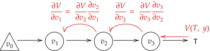
scale datasets and a procedure that aims at minimizing an error function of the network’s prediction with respect to the given target output value. The most commonly used training algorithms share the same pipeline to find a minimum of the error function, defined by a two-stage process [22]. In the first one, the derivatives of the error function with respect to the synaptical weights, the connections among layers, are evaluated. In the latter one, the derivatives are used to compute the adjustment to the architecture parame-ters. In this phase, starting from simple techniques such as gradient descent [23, 24] several powerful optimization schemes have emerged [3]. Going back to the the first stage, derivatives are computed exploiting Automatic Differ-entiation. Using the chain rule of calculus, it is possible to undergo a message passing scheme to propagate the error backward, differentiating through the computational graph. The instantiation of Automatic Differentiation in ar-tificial neural networks is known as BackPropagation [25, 26, 23](see Figure 1.2).

T

Figure 1.2: BackPropagation on the computational graph of ANNs exploit-ing the Chain Rule (in red).

Consequently, in BackPropagation the activation of each unit affects all the descendant neurons in the computational graph. Hence, the weight updates are non-local and rely on upstream layers. The downside of these solutions are high memory consumption, to store intermediate values, and the need to

obey to the aforementioned sequential nature of computations.

1.1

Motivations

Despite the previously highlighted promising characteristics, the ability of the human cognitive system is still far away in many aspects. Deep Neural Net-works still lack in term of conceptual abstraction, causal or relational reasoning as long as many other characteristics of intelligent behaviour.

However, whilst the study of human neurological patterns can foster ad-vances in the computational processes behind artificial intelligence and neural networks, the actual success of deep learning is a direct consequence of math-ematical solutions. Indeed, the chance to develop a mathmath-ematical superstruc-ture, inspired by intuitions similar to the biological ones, could be capable to grasp the underlying laws of the cognitive processes guiding human-like intel-ligence. This direction could leverage the advances in computational systems modeling and, likewise, it could be prone to the injection of interesting and beneficial solutions or shortcuts.

Following the previously presented principles, this dissertation is inspired by a recent line of research that describes learning using the unifying math-ematical notion of “constraint” [27, 28]. This line of research lays the foun-dations for a comprehensive theory for the design of intelligent agents, giving a broader view of learning. In particular, the intuition comes from the con-sideration that just like humans, intelligent agents live and interact with an environment that imposes the fulfillment of several constraints. Therefore, it is possible to build a computational model of learning based on this mathe-matical notion. This approach foster the model ability to process higher level concepts, and in particular to handle the injection of external knowledge on the domain of the task-at-hand.

Complex environments can be modeled as a set of constraints, which the agent is expected to satisfy. As introduced in [29] and then systematically studied in [30], the theory of Learning from constraints takes inspiration from principles of cognitive development and stage-based learning. An agent goes through a first training stage considering only the supervised examples, i.e. sub-symbolic information provided as an input to ouput point–wise constraint.

T

Figure 1.3: The decomposition of the computational graph into local com-ponents, connected via constraints.

In this way, the agent is expected to develop some kind of abstract and higher level cognitive capabilities, following a completely data–driven mechanism. Hence, in principle the agent could be capable to process more abstract and symbolic knowledge, injected into the models through a semantic-based reg-ularization, in the form of constraints to be fulfilled. The symbolic prior knowledge injected in the second stage via constraints is generally represented by logic clauses [31, 30].

The unifying concept of constraint is broadly general and able to manipu-late various kinds of knowledge in different tasks and contexts. For instance, they have been used to enforce the probabilistic normalization when learning density distributions or functions modeling a classification task [32], or to im-pose consistency of the classifier outputs either in the case of different views of the same object [33] or in the case of correlations in time [34]. As it become clear from these examples, all these methods leverage constraints in order to incorporate domain knowledge into the neural models.

The contributions, presented in this thesis, explore a novel path in the direction of learning via the unifying mathematical notion of constraints. The main intuition is the ability to decompose the neural architectures into local components, i.e. subparts constituting the overall architecture, as depicted in Figure 1.3.

Rather than leveraging the constraints to express and inject external knowl-edge onto the domain of the task-at-hand, the intuition is to exploit constraints to force internal knowledge onto the structure of the neural models. The learning problem is enriched with auxiliary local variables whose evolution is constrained to follow the neural computational scheme. Thus, constraints are the mathematical tool leveraged to put into communication the obtained lo-cal structures. In other words, the computation performed by the network is

partially described by structural constraints.

This choice allows us to setup an optimization procedure that is “local”, i.e., it does not require (1) to query the whole network, (2) to accomplish the diffusion of the information, or (3) to bufferize data streamed over time in order to be able to compute gradients.

Learning is the outcome of the interaction of data and constraints, that describe the dependencies in the neural computation. Hence, the proposed technique can be summarized by the definition Learning by Constraints.

1.2

Research questions and contributions

In the following Chapters, given the background overview seen so far, the thesis will explore three different learning settings, seeking to answer the following research questions. These questions are not intended to be self-contained and are characterized by concepts that will be expanded in the next chapters.

In particular, three different learning settings that are instances of the aforementioned scheme will be investigated: (1) constraints among layers in feed-forward neural networks, (2) constraints among the states of neighboring nodes in Graph Neural Networks (GNNs), (3) constraints among predictions over time.

1. BackPropagation has become the de-facto algorithm for training neural networks. Despite its success, the sequential nature of the performed computation hinders parallelizations capabilities and causes a high mem-ory consumption. Is it possible to devise a novel computational method for a generic Directed Acyclic Graph that gets inspiration and advantages from principles of locality?

Constraint-based Neural NetworksIn the proposed approach, Local Propagation, DAGs can be decomposed into local components. The pro-cessing scheme of neural architecture is enriched with auxiliary variables corresponding to the neural units, and therefore can be regarded as a set of constraints that correspond with the neural equations. Constraints enforce and encode the message passing scheme among neural units, and in particular the consistency between the input and the output variables by means of the corresponding weights of the synaptic connections. The

proposed scheme leverages completely local update rules, revealing the opportunity to parallelize the computation.

2. The seminal Graph Neural Networks [35] model uses an iterative con-vergence mechanism to compute the fixed-point of the state transition function, in order to allow the information diffusion among long-range neighborhoods of a graph. Is it possible to avoid such costly procedure maintaining these powerful aggregation capabilities?

Constraining the Information Diffusion in Graph Neural Net-works The original GNN model[35] encode the state of the nodes of the graph by means of an iterative diffusion procedure that, during the learning stage, must be computed at every epoch, until the fixed point of a learnable state transition function is reached, propagating the infor-mation among the neighbouring nodes. Lagrangian Propagation GNNs decompose this costly operation, proposing a novel approach to learning in GNNs, based on constrained optimization in the Lagrangian frame-work. Learning both the transition function and the node states is the outcome of a joint process, in which the state convergence procedure is implicitly expressed by a constraint satisfaction mechanism, avoiding iterative epoch-wise procedures and the network unfolding.

3. Unsupervised learning from continuous visual streams is a challenging problem that cannot be naturally and efficiently managed in the clas-sic batch-mode setting of computation. Lifelong learning suffers from the problem of catastrophic forgetting [36]. Hence, the task of transfer-ring visual information in a truly online setting is hard. Is it possible to overcome this issue by devising a local temporal method that forces consistency among predictions over time?

Constraint-based Mutual Information Computation in Salient Areas of Video StreamsWe consider the problem of transferring in-formation from an input visual stream to the output space of a neural architecture that performs pixel-wise predictions. This problem consists in maximizing the Mutual Information (MI) index. Most approaches of learning commonly assume uniform probability density of the input. Actually, devising an appropriate spatio-temporal distribution of the

vi-sual data can foster the information transfer. In the proposed approach, a human-like focus of attention model takes care of filtering the spa-tial component of the visual information, restricting the analysis on the salient areas. On the other side, various temporal locality criteria can be explored. In particular, the analysis sweeps over the probability es-timates obtained in subsequent time instants. Global changes in the entropy of the output space are approximated by introducing a specific constraint. The probability predictions obtained at each time instant can once more be regarded as local components, that are put into rela-tion by soft-constraints enforcing a temporal estimate not limited to the current frame.

To sum up, the proposed scheme decomposes neural architectures into lo-cal subparts, i.e. neural network neurons (or layers), node states updates in graphs, or time instant predictions, obtained via the introduction of local aux-iliary variables. Constraints are the mathematical tool leveraged to put into communication these components, connecting units, aggregating neighboring nodes in graphs, forcing temporal entropy predictions, respectively.

In such a way, several advantages like parallelization and locality of com-putations are obtained, besides the ability to avoid costly procedures without sacrificing representational capabilities.

1.3

Thesis structure

In the following Chapters the thesis will try to answer the research questions described in Section 1.2, preceded by a general description of the theoretical foundations.

1. Chapter 2 gives a broad introduction to all the concepts this disser-tation is based on. Some insight on artificial neural architectures are followed by an introduction to optimization schemes, with a focus on BackPropagation. Moreover, we recall some backgrounds of a theoret-ical framework for BackPropagation, as long as constrained differential optimization based on the Lagrangian Framework. This principles will establish the foundation for the following Chapters.

2. In Chapter 3, constrains are defined among layers in feed-forward neu-ral networks and potentially over arbitrary Directed Acyclic Graphs, obtaining the Local Propagation optimization procedure. Based on [37]. 3. In Chapter 4, the iterative diffusion mechanism defining the message passing scheme of Graph Neural Networks is defined via constraints. Based on [38, 39]

4. Finally, in Chapter 5 a lifelong online learning process in visual streams is empowered by constraints among predictions over time. Based on [40]

1.4

List of Publications

In the following, a list of the research contributions produced during the period of this research is provided.

Peer reviewed conference papers

1. Tiezzi, M., Melacci, S., Betti, A., Maggini, M., and Gori, M. (2020). “Focus of Attention Improves Information Transfer in Visual Features”. Advances in Neural Information Processing Systems, 33. (NeurIPS 2020)

Candidate Contribution: joint definition of the method, joint design and implementation of both the framework and the experiments. 2. Meloni, E., Pasqualini, L., Tiezzi, M., Gori, M., and Melacci, S. (2020).

“SAILenv: Learning in Virtual Visual Environments Made Simple”. In International Conference on Pattern Recognition (ICPR 2020)

Candidate Contribution: definition of the theory, joint definition of the method, design and implementation of the experiments.

3. Tiezzi, M., Marra, G., Melacci, S., Maggini, M., and Gori, M. (2020). “A Lagrangian Approach to Information Propagation in Graph Neural Networks”. In European Conference of Artificial Intelligence (ECAI 2020)

Candidate Contribution: joint definition of the theory, joint defini-tion of the method, design and implementadefini-tion of both the framework and the experiments.

4. Marra, G., Tiezzi, M., S. Melacci, A. Betti, Maggini M. and M. Gori. (2020) “Local Propagation in Constraint-based Neural Networks”. In In-ternational Joint Conference on Neural Networks (IJCNN2020): 1-8. Candidate Contribution: formulation of the solution, design and de-velopment of the experimental campaign

5. Tiezzi, M., Melacci, S., Maggini, M., and Frosini, A. (2018, October). “Video Surveillance of Highway Traffic Events by Deep Learning Ar-chitectures”. In International Conference on Artificial Neural Networks (ICANN 2018) (pp. 584-593). Springer, Cham.

Candidate Contribution: joint formulation of the problem, formula-tion of the soluformula-tion and design of the experimental campaign.

Workshop papers

1. Tiezzi, M., Marra, G., Melacci, S., Maggini M. (2020) “Deep La-grangian Propagation in Graph Neural Networks”. In Graph Represen-tation Learning and Beyond (GRL+ ICML 2020 Workshop) . Candidate’s contributions: joint definition of the theory, joint defi-nition of the method, design and implementation of both the framework and the experiments.

2. Tiezzi, M., Marra, G., Melacci, S., Maggini M., and Gori M. (2020) “Lagrangian Propagation Graph Neural Networks” In Deep Learning on Graphs: Methodologies and Applications (DGLMA- AAAI 2020 Workshop) .

Candidate’s contributions: joint definition of the theory, joint defi-nition of the method, design and implementation of both the framework and the experiments.

3. Zugarini A., Tiezzi, M., Maggini M., (2020) “Vulgaris: Analysis of a Corpus for Middle-Age Varieties of Italian Language”, Seventh Work-shop on NLP for Similar Languages, Varieties and Dialects(VarDial

2020),pages:150–159,

Candidate’s contributions: corpus creation, joint statistical analysis of the corpus, joint design of the experiments

4. Rossi, A., Tiezzi, M., Dimitri, G. M., Bianchini, M., Maggini, M., and Scarselli, F. (2018, September). “Inductive–transductive learning with graph neural networks”. In IAPR Workshop on Artificial Neural Net-works in Pattern Recognition (ANNPR 2018)(pp. 201-212). Springer, Cham.

Candidate Contribution: joint design, development and testing of the overall framework

Papers under review

1. Tiezzi, M., Marra, G., Melacci, S., Maggini M. (2020) “Deep Constraint-based Propagation in Graph Neural Networks”. Submitted at TPAMI Candidate’s contributions: joint definition of the theory, joint defi-nition of the method, design and implementation of both the framework and the experiments.

Neural Network Architecture as Constraints

In the context of Deep Learning, artificial neural architectures are charac-terized by a computational structure that can be generally decomposed into local subcomponents, at different granularity levels. The atomic computa-tional component is the neuron itself, but, at a coarse grain level, appropriate aggregations of neural units, such as layers, can be considered as building blocks of a complex architecture. The idea is to describe the interactions of these blocks thanks to the introduction of local auxiliary variables and the mathematical tool of constraint, which is leveraged in order to define and de-scribe the connections among such submodules. This intuition imply several advantages, allowing to express a local processing scheme in several archi-tectures (Chapter 3), to avoid costly iterative procedures (Chapter 4) or to better estimate certain temporal quantities (Chapter 5). The backbone of this approach is the ability to describe the flow of information happening inside computational models by means of constraints.

In this Chapter we will establish a common notational framework, provide the necessary background and give a comprehensive overview of the needed background methods. In what follows, we will give an introduction to several Artificial Neural Networks (ANNs) in Section 2.1 and the learning procedure commonly used in ANNs in Section 2.2. Afterward, a brief introduction on the Lagrangian formalism for constrained Optimization will be given in Sec-tion 2.4, followed by the descripSec-tion of methods to carry on optimizaSec-tion in this context in Section 2.6, and by insights on a Lagrangian derivation of BackPropagation in Section 2.5.

2.1

Artificial Neural Architectures

Artificial Neural networks (ANN) are machine learning models born as a byproduct of studies on the information processes happening in biological neu-rons [15, 16, 17, 18]. At their core, they are composed of simple interconnected processing units known as artificial neurons, connected by synaptic weights, which are commonly denoted with the symbol w and represent learnable pa-rameters defining the overall computation. The final goal is the approximation of some function of the input x, a mapping y = f(x; w), where the param-eters w are learned in order to achieve the best input to output fitting on a set of given examples. Such mapping is obtained via the composition of many simple functions, defined by each artificial neuron. The overall computation emerges from the flow of information in the network of neurons, given the pat-tern of connections between them and the synaptic weights assigned to such connections.

Generally speaking, the flow of information happening inside ANNs can be described in terms of a computational graph G = (V, E), a Directed Acyclic Graph that describes any program or computable function as a composition of elementary functions. The computation consists in a data flow through the edges E, undergoing several subsequent numerical transformations. Each node v ∈ V represents an input (scalar, vector, matrix, tensor, etc.) or an intermediate variable (neural activation) obtained by applying elementary op-erations (e.g. non-linearities, tensor multiplications) to the values available at another node connected to v by an arc e ∈ E. A set of neurons residing at the same depth – layer – of the data-flow are denoted by the same node vi (see

top of Figure 2.1). Multi-layered (“deep”) neural networks are graphs having more than two of such layers.

Several neural architectures have been developed in order to deal with different tasks. In the following, we will briefly review the main models that will be used in the dissertation.

2.1.1 Multi-Layer Perceptrons

MLPs represent a powerful instance of the previously mentioned computa-tional DAG, as depicted in Figure 2.1. In particular, it is a directed

feed-T

T

Figure 2.1: Instance of the computational graph (top) as a Multi–Layer Perceptron (bottom). A set of neurons at the same depth – layer – of the data-flow are denoted by the same node vi. To ease the plot comprehension,

we depict an MLP with sparse connections among neurons.

forward data-flow graph. Each artificial neuron receives an input vector x ∈ Rn, which may be a task related fixed-size external input or the intermedi-ate outputs of the set of neurons in the parent nodes of the computational graph. Given this vector, the neuron computes a linear combination of its components parametrized by a weight vector w ∈ Rn_{and it finally adds a bias}

value b. This procedure computes the so called neural activation, on which an activation function σ(·) can be applied, in order to obtain the unit output y ∈ R : y = σ( n ∑︂ i=1 wixi+ b) = σ(W xT) (2.1)

where W and x collect the connection weights and the input variables, respectively, including also the bias in W in correspondence to an additional input entry in x set to a constant value of 1.

MLPs assume a feedforward structure in which several neural units sharing the same input compose a layer, and several of such layers are stacked, yielding the overall architecture. The term “feedforward” refers to the fact that data flow in the same direction, processed in a synchronous way, starting from the input layer up to the output layer, through the hidden layers. In general each unit populating a layer is connected to all the neural units composing

the following one, in a fully-connected topology. Given a vectorial form of the input signal x0, where the subscript denotes the layer index, the computational

graph can be translated into a series of dense matrix multiplications, regarded as matrix form of the computation. The output of a generic hidden layer ℓ ∈ [1, H] is indicated with xℓ, that is a column vector with a number of

components equal to the number of hidden units in such layer. We also have that

xℓ = σ(Wℓ−1xℓ−1) (2.2)

where σ(·) is the activation function that is intended to operate element-wise on its vectorial argument (we assume that this property holds in all the following functions). The matrix Wℓ−1 collects the weights linking layer ℓ − 1

to ℓ. We avoid introducing bias terms in the argument of σ(·), to simplify the notation (they can be included in the considered variables as stated before). Activation functions

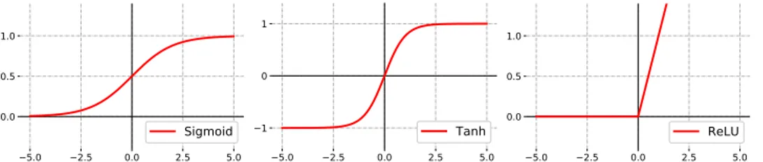
In literature, several activation functions σ(·) have been introduced. This dissertation exploits the following mappings, depicted in Figure 2.2:

• Logistic Sigmoid – A Monotonic continously differentiable mapping from R to [0, 1]

σ(a) = 1

1 + e−a (2.3)

• Hyperbolic Tangent – A Sigmoidal shape mapping from R to [−1, 1]

σ(a) =tanh(a) (2.4)

• Rectified Linear – A mapping defined as the positive part of its argu-ment

σ(a) =max(0, a) (2.5)

2.1.2 Recurrent Neural Networks

Whilst MLPs are designed to process fixed sized inputs, several problems require an architecture able to handle streams of data, potentially having

5.0 2.5 0.0 2.5 5.0 0.0 0.5 1.0 Sigmoid 5.0 2.5 0.0 2.5 5.0 1 0 1 Tanh 5.0 2.5 0.0 2.5 5.0 0.0 0.5 1.0 ReLU

Figure 2.2: The mapping defined by the Sigmoid, Hyperbolic Tangent (Tanh) and Rectified Linear Unit (ReLU) activation functions.

variable-length. The main idea behind Recurrent Neural Networks (RNNs) [41, 42] is to extend neural networks to sequentially structured data, by gener-ating a dynamic computational graph capable to unroll on the length of each individual input sequence. The unfolding of the computational graph allows us to compute a hidden representation for each time step, i.e. node, based on the current input and the node’s previous state.

Formally speaking, given an input sequence Ä

x(0)₀ , x(1)₀ , .., x(T )₀ ä composed by T steps, x(i)

0 denotes the input at the i-th time step. A layered RNN

computes the state vector for layer ℓ at time step t as:

x(t)_ℓ = σ(Wℓ−1x(t)_ℓ−1+ Uℓx(t−1)_ℓ ) (2.6)

where Uℓ is the matrix of the weights that tune the contribution of the

state at the previous time step. The initial state x(0)

ℓ is generally set to zero.

As can be seen from Eq. (2.6), this model exploits a temporal weight sharing, meaning that the same learnable parameters are exploited at the different time steps.

2.1.3 Convolutional Neural Networks

Convolutional Neural Networks (CNNs) [43] are feed-forward architectures exploiting peculiar operations in one or more sub-parts of the computational graph, in particular convolution and pooling.

The main reason behind the introduction of the convolution operation is the ability to apply the same parametrized function - called kernel - to dif-ferent areas of the input, in order (1) to deal with high dimensional data

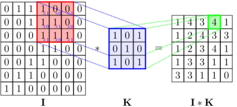
0 1 1 1 0 0 0 0 0 1 1 1 0 0 0 0 0 1 1 1 0 0 0 0 1 1 0 0 0 0 1 1 0 0 0 0 1 1 0 0 0 0 1 1 0 0 0 0 0 I ∗ 1 0 1 0 1 0 1 0 1 K = 1 4 3 4 1 1 2 4 3 3 1 2 3 4 1 1 3 3 1 1 3 3 1 1 0 I ∗ K 1 0 1 0 1 0 1 0 1 ×1 ×0 ×1 ×0 ×1 ×0 ×1 ×0 ×1

Figure 2.3: 2D convolution of an input tensor I and a kernel K (Figure thanks to Petar Veličković).

and (2) to extract common patterns from heterogeneous locations of the in-put raster. Indeed, processing an inin-put signal (e.g. an image) encoded by a tensor of dimension c × h × w (number of channels, height and width of the image, respectively) is an expensive task for a common MLP, requiring full connectivity between each pixel (input element) and every hidden unit, resulting in a complexity of O(c × h × w) for each hidden unit. Moreover, a fully connected network will be needed to learn translation invariance from the examples, whereas the convolution operation can guarantee this property a priori. In fact, thanks to the kernel sharing property, convolutional layers are equivariant to translation, practically meaning that they are able to produce the same output when detecting the same pattern in different locations.

In the simplest case the convolution operation can be defined for an 1-dimensional vector input x0 ∈ Rn. In this case, the convolutional kernel is a

vector K ∈ Rk _{of learnable parameters, where k < n, that slides along the}

input with a given stride. At each position, the kernel is multiplied element-wise with the k input components around the current element, then summed up producing an aggregated scalar value. The newly obtained values com-pose a feature map. Generally, many Kernels slide over the same locations, obtaining an output composed by many channels. This same concept can be easily extended to multi-dimensional tensors, for instance an input image X ∈ Rc×h×w[43]. See Figure 2.3 for a graphical representation. Typically, non-linearities are applied after convolutional layers.

Another relevant component of CNNs are Pooling layers, that aggregate (summing up, averaging or extracting the maximum) the values computed by the convolution filters in small sub-regions (e.g. 2 × 2) of the input feature map to yield a single output. Pooling performs a sub-sampling in the feature maps and, hence, helps reducing the potentially redundant information and the memory consumption, allowing to increase the channel size to obtain a higher representational power in higher level features. Moreover, by pooling the CNN gains the property of translation invariance to small displacements that is useful if we care more about the presence of some features rather than their exact location.

Residual Networks

With very deep neural networks the increased representational power comes at the cost of a higher difficulty in the training procedures. Indeed, stacking many layers of computation interleaved with sigmoidal activation functions σ(·), hinders the backpropagation of error signals, as we will see in Section 2.2, a problem known with the term vanishing gradient.

ResNets [44] consist of several stacked residual units, that are robust with respect to the vanishing gradient problem. In particular, this solution has been shown to attain state-of-the art results in Deep Convolutional Neural Nets [44] (without being limited to such networks).

The most generic structure of a residual network [45] is defined by layers whose outputs are computed by

xℓ = z(h(xℓ−1) + f (Wℓ−1xℓ−1)) . (2.7)

In [44], z(·) corresponds to a rectifier (ReLu) and h(·) is the identity function, while f(·) is a non-linear function. The role of the residual or skip connection is to create an alternative path, a shortcut h(xℓ−1), for the flow of information

coming from the previous layer. In this way, this information can directly be propagated, whereas the role of the current layer becomes to solely learn a residual function f(Wℓ−1xℓ−1).

2.1.4 Graph Neural Networks

The architectures described in the previous sections have been devised to extend the representation capability of ANNs beyond flat vectors of features. Recurrent Neural Networks [41, 42] have been proposed to process sequences, Convolutional Neural Networks to deal with groups of adjacent pixels [46].

However, several tasks require to deal with data that exhibit a complex structure, for instance data can be provided as entities and relations among them. Such data can generally be represented by a graph G = (V, E), where V is a finite set of nodes and E ⊆ V × V collects the arcs, representing relations between an ordered pair of nodes (i, j) ∈ V × V .

Several attempts were made to deal with such Non-Euclidean structures [47], also restricting the problem domain to directed acyclic graphs (Recursive Neural Networks [48, 49]).

The term Graph Neural Network (GNN) refers to a general computational model, that exploits the inference and learning schemes of neural networks to process non Euclidean data, organized as graph structures. GNNs, with a procedure that resembles Recursive networks, dynamically unfold their com-putational graph on the topology of the whole input structure. They are able to take into account both the local information attached to each node and the whole graph topology. GNNs can implement either a node-focused function, where an output is produced for each node of the input graph, or a graph-focused function, where the representations of all the nodes are aggregated to yield a single output for the whole input graph.

Message Passing Neural Networks

Inspired by the original model [35], Graph Representation Learning is becom-ing one of the hottest topic in Deep Learnbecom-ing, thanks to hundreds of works in this direction. The work by Gilmer [50, 51] is an effort to unify this entire movement under the common framework of Message Passing NNs (MPNNs). Each node i is characterized by an initial set of features, denoted by li (label

in the original model). The same holds for an arc connecting node i and j, whose feature, if available, is denoted with l(i,j). Each node i has an associated

hidden representation (or state) xi∈ Rs, which in modern models is initialized

passing scheme among neighboring nodes, denoted by Ni or ne[i], followed

by an aggregation of the exchanged information, to obtain the updated node representation x(t+1) i : x(t)_(i,j)= MSGt(x(t)_i , x(t)_j , l(i,j)) (2.8) x(t+1)_i = AGGt(x(t)_i ,∑︂ j∈Ni x(t)_(i,j), li) (2.9)

where x(i,j) is an explicit edge representation, i.e. the exchanged message,

computed by a learnable mapping MSGt_{(·). The mapping AGG}t_{(·)aggregates the}

messages from incoming edges to node i, exploiting also local node informa-tion (state and features). The funcinforma-tions MSGt_{(·) and AGG}t_{(·) are typically}

im-plemented via MLPs, whose parameters (weights) are learned from data, and shared among nodes in order to gain generalization capability and save mem-ory consumption. Generally these two functions are not shared between mes-sage passing steps, hence MSGt_{(·) denotes the message function implemented}

at time step t. This choice entails both a higher representational capability and an increased memory and computational complexity in the prediction. Such steps are commonly referred to as layers, hence an ℓ-step message pass-ing scheme can be seen as a ℓ-layered graph network. Havpass-ing ℓ-layers, such model is able to directly propagate a message up-to an ℓ-hop distance. The representation of each node at the top layer represents the node-level output of the GNN.

The Graph Neural Network Model

For the purpose of this dissertation we focus our attention on the seminal model by Scarselli et al. [35], which can be seen as a particular instantiation of MPNNs with peculiar characteristics. The node states xi ∈ Rs are an

ad-ditional variable to the problem, independent from the node initial features li∈ Rm. The node states are zero-initialized, and the node state update

func-tion, denoted with the term state transition function fa(·), is conditioned on

neighboring states xj with j ∈ Ni and local node features. As described from

the MPNNs guidelines, the state of node i is the outcome of the iterative ap-plication of the shared state transition function computation, which processes

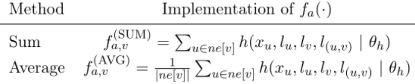
Method Implementation of fa(·)

Sum fa,v(SUM) =∑︁_u∈ne[v]h(xu, lu, lv, l(u,v) | θh)

Average f(AVG)

a,v = _|ne[v]|1 ∑︁u∈ne[v]h(xu, lu, lv, l(u,v) | θh)

Table 2.1: Common implementations of the state transition function fa().

The function h() is implemented by a feedforward neural network with s out-puts, whose input is the concatenation of its arguments.

information attached to each node and to its neighborhood. However, dif-ferently from layered-MPNNs, in this case the same state transition function is used for every node and for every iteration or aggregation step. The final purpose is the computation of a vector embedding for each node

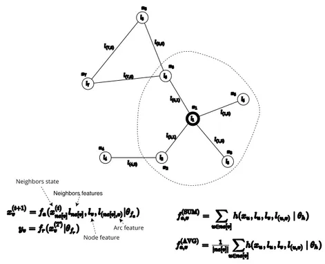
x(t+1)_v = fa(x(t)_ne[v], lne[v], lv, l(ne[v],v)|θfa) (2.10) where ne[v] are the neighbors of v and lv, lne[v] ∈ Rm, l(ne[v],v) ∈ Rd

en-code additional information (sometimes referred as labels) on the node v, on its neighbors and on the arcs connecting them. The vectors θfa collect the function parameters (i.e. the weights of the neural networks implementing the functions) that are adapted by the learning procedure.

It should be noted that the state transition function fa(·)may depend on

a variable number of inputs, given that the nodes v ∈ V may have different degrees de[v] = |ne[v]|. It is for this reason that the authors proposed the implementations reported in Table 2.1 and represented in Figure 2.4, that inspired the arc-level message passing scheme of MPNNs.

The h(·) function, commonly implemented by an MLP, acts at arc-level receiving as input the concatenation of its arguments (for example, in the first case the input consists of a vector of s + 2m + d entries, with l(u,v)∈ Rd and

lu ∈ Rm). The plain aggregation of the arc-level messages yields the node

state at the current iteration. Another interesting property of such functions is the invariance with respect to permutations of the nodes in ne[v], unless some predefined ordering is given for the neighbors of each node.

Once the state transition function application has been iterated T times, GNNs employ a readout output function, whose nature depends on the task at hand, by leveraging the final node states x(T )

i , as yv = fr Ä x(T )_v | θ_frä, (2.11a) yG = fr Ä {x(T )_v , v ∈ V } | θfr ä , (2.11b)

where yv is the node level output in the node-focused case, whereas yG is

the graph level output in the graph-focused case. The vectors θfr collect the weights of the neural networks implementing the readout function. The state transition function fa(·) is recursively applied on the graph nodes, yielding

an information diffusion mechanism whose range depends on T . In fact, by stacking t times the aggregation of 1-hop neighborhoods by fa(·), a node is

able to directly receive messages coming from nodes that are distant at most t-hops.

To draw a parallel with MPNNs, the number t may be seen as the depth of the GNN and thus each iteration can be considered a different layer of the GNN. In this case, however, all the layers (i.e., iterations) share the same fa(·). Furthermore, this same function is computed leveraging at each time

step the initial node features, potentially avoiding oversmoothing or washing away node feature information [52].

Given these considerations, a sufficient number of layers seems the key to produce a node state informed of the whole graph topology. In the original GNN model [53], Eq. (2.10) is iterated until convergence of the state repre-sentation, i.e. until x(t)

v ≃ x(t−1)v , ∀v ∈ V. This scheme corresponds to the

computation of the fixed point of the state transition function fa(·) on the

input graph. As stated by the Banach fixed-point theorem, in order to guar-antee the convergence of this phase, the transition function is required to be a contraction map [54].

2.2

Learning by BackPropagation

Deep Neural Nets are usually trained leveraging a procedure that aims at op-timizing a differentiable loss function, denoted by V (·), which gives a measure

Neighbors state

Neighbors features

Node feature Arc feature

Figure 2.4: The Graph Neural Network model. of how good are the prediction capabilities of the current model.

As briefly mentioned in Chapter 1, the common training pipeline is com-posed by a two-stage process aiming at the optimization of the loss function [22]. In the former phase the derivatives of the error function with respect to the weights, which we denote with ∇wV, are evaluated. In the latter

phase, advanced optimization schemes, inspired by gradient descent [23, 24], are employed to adjust the network parameters towards values yielding an improvement of the performances [3].

The first stage of this process, i.e. the parameters derivative computa-tion, leverages Automatic Differentiation techniques and the data-flow com-putational model of ANNs presented in Section 2.1. The instantiation of Automatic Differentiation in neural networks is known as BackPropagation [25, 26, 23], which has become the "de-facto" standard to compute derivatives (as sketeched in Figure 2.5).

T

Figure 2.5: BackPropagation on a generic computational graph exploiting the Chain Rule (in red).

In the following, without any loss of generality, we will show the derivation of the BackPropagation algorithm (BP) in a supervised setting, where we are given N supervised pairs (x0,i, yi), i = 1, . . . , N, where x0,i and yi denote

the input features and the target values of the i-th example, respectively. Moreover, we consider a Multi Layer Perceptron (MLP) with H hidden layers as an instantiation of a generic neural architecture described by a Directed Acyclic Graph (DAG), following the notation introduced in Section 2.1.

If we denote the prediction of the model for the pattern i with with y′ i =

σ(WHxH,i), the function V (yi, yi′) computes the loss on the i-th supervised

pair, and, when summed up for all the N pairs, it yields the objective function that is minimized by the learning algorithm. In the case of classic neural networks, the variables involved in the optimization are the weights Wℓ, ∀ℓ.

Without any loss of generality, we will refer to the Squared Error cost function: VSE= 1 2 N ∑︂ i=1 (yi− y′i)2 (2.12)

The goal is the computation of the derivative of the loss function with respect to the weights. Firstly, we consider the evaluation of the loss function derivative with respect to the weight matrix WH, collecting the weights linking

layer H to the output layer, which will be denoted as H + 1. ∂V ∂WH = N ∑︂ i=1 ∂(1₂(yi− y′i)2) ∂WH = − N ∑︂ i=1 (yi− yi′) ∂y_i′ ∂WH (2.13)

The last term can be computed exploiting the chain rule ∂y_i′ ∂WH = ∂σ(WHxH) ∂WH = ∂σ(WHxH,i) ∂WHxH,i ∂WHxH,i ∂WH = σ′(WHxH,i)xTH,i (2.14) Hence, we obtain ∂V ∂WH = − N ∑︂ i=1 (yi− yi′)σ′(WHxH,i)xTH,i (2.15)

We introduce the notation

δH+1= (yi− y′i)σ ′

(WHxH,i) (2.16)

where δi are commonly referred to as errors. Substituting it into Eq.

(2.15), we obtain ∂V ∂WH = − N ∑︂ i=1 δH+1xTH,i (2.17)

Subsequently, we evaluate the derivative of the loss function with respect to the weights of the underneath layer, WH−1, obtaining:

∂V ∂WH−1 = N ∑︂ i=1 ∂(1₂(yi− y_i′)2) ∂WH−1 = − N ∑︂ i=1 (yi− yi′) ∂y_i′ ∂WH−1 (2.18)

We evaluate the derivative of the last term using once again the chain rule ∂y′_i ∂WH−1 = ∂σ(WHxH,i) ∂WHxH,i ∂WHxH,i ∂WH−1,i = σ′(WHxH,i)WHT ⊙ ∂xH,i ∂WH−1,i (2.19)

where, exploiting one last time the chain rule: ∂xH,i ∂WH−1,i = ∂σ(WH−1xH−1,i) ∂WH−1,i = ∂σ(WH−1xH−1,i) ∂WH−1xH−1,i ∂WH−1xH−1,i ∂WH−1 = = σ′(WH−1xH−1,i)xTH−1,i

Substituting into Eq. (2.18) we obtain − N ∑︂ i=1 (yi− y′i)σ ′ (WHxH,i)WHT ⊙ σ ′ (WH−1xH−1,i)xTH−1 (2.20)

Leveraging Eq. (2.16) we define the error of the current layer as

δH = (δH+1WHT) ⊙ σ′(WH−1xH−1,i) (2.21)

and finally we get, substituting into Eq. (2.20) ∂V ∂WH−1 = − N ∑︂ i=1 δHxTH−1 (2.22)

This results can be generalized to the derivative computation of a generic layer ℓ : ∂V ∂Wℓ−1 = − N ∑︂ i=1 δℓ,i· xTℓ−1,i, δℓ,i = σ′(Wℓ−1xℓ−1,i) ⊙ Ä W_ℓTδℓ+1,i ä , (2.23) that are the popular equations for updating weights and the Backpropa-gation deltas.

From Eq. (2.23) it is quite clear the dependence of the BP algorithm on the sequential nature of the computations. The weight derivatives are obtained thanks to the backward propagation of the errors δifrom the uppermost layers.

In order to compute the derivatives of the loss function with respect to the early layers weights, it is necessary to backpropagate the errors through all the subsequent layers. Thus, in this sense BP is a Non-local algorithm.

The derivatives of the network parameters are exploited into the second stage of the learning process mentioned at the beginning of this section, the update of the network parameters. Techniques such as Stochastic Gradient Descent (SGD) operate in learning epochs. In each of them, firstly a mini-batch, a subset of training examples, is used to evaluate the loss function and then compute all the weight gradients through BP. Afterwards, the model

parameters are updated moving towards the minima of the loss function, along the direction of the descent of the gradient :

∆Wt+1= Wt− η∇_WtV (·) (2.24)

where η denotes the update pace or learning rate [22]. 2.2.1 Learning in Structured Networks

The end-to-end differentiation capability characterizing the BackPropagation algorithm fosters its application to several kinds of architectures and meth-ods. While the CNNs data-flow can be simply translated into a feed-forward one and directly dealt with by an extension of BP, that takes into account the propagation of the errors through the pooling operator, the application to structured dynamical architectures such as RNNs or GNNs is not straight-forward. In the context of recurrent structures, the recursive definition of the update equation introduces loops into the network computational graph, that is in practice unrolled in time along the input sequential structure to be processed. This method allows us to define the BackPropagation Through Time (BPTT) algorithm [18]. The recurrent layer is unfolded many times as the number of time steps to be processed, with each step sharing the same parameters. For this reason, the total gradient is given by accumulating of the gradients computed at each time step.

The same consideration holds for the GNN model [35], whose convergence procedure up to the fixed point of the state transition function shares a dy-namical unrolling procedure similar to that of RNNs, backpropagating the gradient errors on the GNN unfolded following the graph topology. For this reason this model in recent surveys falls under the umbrella of Recurrent GNNs (RecGNNs).

One interesting consideration in the context of learning in very deep net-works via BackPropagation is the vanishing gradient problem. Applying recur-rent architectures to long sequences implies the creation of very deep unrolled networks. When using BPTT, due to the usage of the chain rule and Eq. (2.23), the computation of the gradients at a given time step depends on the propagation of the error through all the subsequent steps, that implies the multiplication by the network output derivative at each step. The usage of

non-linearities, whose output belongs to a limited range (0, 1) with a satu-rating behaviour, such as the sigmoid, results in the product of many small values, that causes a quick decay of the error signal towards zero. Hence, the term vanishing gradient has been used to enlighten the fact that the contri-bution of early steps of the unrolled computational graph is quite likely to become negligible.

The introduction of the ReLU activation function can alleviate this prob-lem, but also affects very deep networks with the opposite issue of exploding gradients, caused by the same gradient product diverging due to the unre-stricted function output space.

2.2.2 Complexity Analysis

The success of the Backpropagation algorithm is mostly due to its ability to perform the gradient computation in a very efficient manner. In particular, the forward flow of information inside the model, for a single input pattern, is dominated by the weight matrices products needed for the neural activation computation, resulting in a O(|W |) complexity.

The same applies for the backward pass, where once again the weight ma-trices are leveraged in order to backpropagate the δℓ, resulting in the same

complexity of O(|W |). All the competing methods, such as computing deriva-tives by finite differences, require a greater computational complexity.

In the context of the GNN learning procedure, there are synchronous up-dates among all nodes and multiple iterations for the node state embedding, with a computational complexity for each parameter update of O(T (|V | + |E|)), where T is the number of iterations, |V | the number of nodes and |E| the number of edges [35].

2.3

Regularization

The usage of mapping functions parametrized by many learnable variables favours the creation of separating hyperplanes that highly adapt to the lower dimensional manifolds populated by the input patterns, somehow memoriz-ing the characteristics of the trainmemoriz-ing data. However, such behaviour may hinder the generalization capabilities of the model. Deep Neural Nets, often

constituted by million of parameters, deeply suffer from this overfitting issue, and often the trained models are not capable to generalize satisfactorily their performance to the test data. In order to alleviate overfitting, some regular-ization methods have been devised, that extend the learning problem with additional soft-constraints that guide the optimization process restricting the set of allowed parameters, thus limiting their degrees of freedom.

For the purpose of this Thesis, two methods will be exploited, given the learnable parameter vector w and the loss function V (·):

L1-norm regularizer Reduces the parameters search space adding a

penalty, weighted by α > 0, in order to help the model to focus on a smaller number of paths. The loss function is transformed:

Vˆ (·) = V (·) + α∥w∥ (2.25)

L2-norm regularizer The parameters are softly enforced to not diverge

from zero, avoiding any excessive adaptation to the training data, transforming the loss function:

Vˆ (·) = V (·) + α 2∥w∥

2 _(2.26)

This regularizer leads to the weight decay scheme.

2.4

The Lagrangian formalism

In the previous Sections, various Neural Network architectures and their learn-ing mechanisms have been described via the unifylearn-ing concept of computational graph model. Each one of the submodules constituting such graph, i.e. each node vi∈ V from G = (V, E), can be seen as an independent component in the

data-flow. Therefore, in the following Chapters neural architectures will be treated as a collection of submodules, whose interconnection and processing scheme is defined via constraints. This entails several advantages in the com-putational, memory and learning point of view. The information data flow happening in the networks computational graph will be defined in the con-text of constraint satisfaction. In order to deal with constrained optimization, many techniques have been explored [55].