A simulation study on two analytical techniques for alternating treatments designs
Rumen Manolov
Department of Social Psychology and Quantitative Psychology,
Faculty of Psychology, University of Barcelona (Spain)
Author Note
Correspondence concerning this article should be addressed to Rumen Manolov, Departament de
Psicologia Social i Psicologia Quantitativa, Facultat de Psicologia, Universitat de Barcelona, Passeig de la Vall d’Hebron, 171, 08035-Barcelona, Spain. Telephone: +34934031137. E-mail:
Abstract
Alternating treatments designs (ATDs) are single-case experimental designs entailing the rapid
alternation of conditions and the specific sequence of conditions is usually determined at
random. The visual analysis of ATD data entails comparing the data paths formed by connecting
the measurements from the same condition. Apart from visual analyses, there are at least two
quantitative analytical options also comparing data paths. On option is a visual structured
criterion (VSC) regarding the number of comparisons for which one conditions has to be
superior to the other in order to consider that the difference is not due only to random
fluctuations. Another option, denoted as ALIV, computes the mean difference between the data
paths and uses a randomization test to obtain a p value. In the current study, these two options
are compared, along with a binomial test, in the context of simulated data, representing ATDs
with a maximum of two consecutive administrations of the same condition and a randomized
block design. Both VSC and ALIV control Type I error rates, although these are closer to the
nominal 5% for ALIV. In contrast, the binomial test is excessively liberal. In terms of statistical
power, ALIV plus a randomization test is superior to VSC. We recommend that applied
researchers complement visual analysis with the quantification of the mean difference, as per
ALIV, and with a p value whenever the alternation sequence was determined at random. We
have extended an already existing website providing the graphical representation and the
numerical results.
Key words: single-case designs, alternating treatments design, Type I error, statistical power, autocorrelation
Introduction
Alternating treatments designs (ATD) are a type of single-case experimental designs (SCED)
that allow for rapid changes in the conditions in which the target behavior is measured.
According to reviews of published SCED studies, ATDs represent approximately 6% to 16% of
the designs used (Hammond & Gast, 2010; Shadish & Sullivan, 2011; Smith, 2012). Moreover,
ATDs are similar to the N-of-1 trials used in health research (Carriere, Li, Mitchell, & Senior,
2015), as they include several alternations from an A (baseline) phase to a B (intervention) phase
and also in reversed order. The main characteristics of ATDs have been dealt with extensively
elsewhere (Barlow & Hayes, 1979; Wolery, Gast, & Ledford, 2014). One of the main features
that we will focus on here is the possibility to determine the sequence of conditions at random. In
case randomization is used, we could distinguish three kinds of design: (a) ATDs defined as
completely randomized designs allow any sequence of conditions (e.g., AAABBBBBAA); (b)
ATDs including randomized blocks, also called sometimes randomized block designs, entail
choosing at random the first condition in a pair of conditions (e.g., AB-BA-AB-AB-BA); and (c)
ATDs including restricted randomization (Onghena & Edgington, 1994), in which the sequence
can contain a maximum of two consecutive administrations of the same condition (e.g.,
AABBABBAAB). For this latter type of ATDs, the restriction mentioned is the most common
one (Heyvaert & Onghena, 2014; Kratochwill et al., 2013; Wolery et al., 2014). Regarding the
requirements for ATDs, a minimum of five repetitions of the alternating sequence has been
suggested (Kratochwill et al., 2010), which entails and is well-aligned with the need for at least
five measurement occasions per condition (Kratochwill et al., 2010; Wolery et al., 2014).
obtained in a previously performed review of published ATD literature (Manolov & Onghena,
2017): the median of measurements per condition was 5.5, whereas the mean was 6.64.
In terms of data analysis, visual inspection is suggested as a first choice (Barlow, Nock, &
Hersen, 2009), but there have also been proposals for using quantifications. Actually, a recent
review of published ATD research (Manolov & Onghena, 2017) revealed that most studies
compute the difference between the means of the conditions compared, as well as a measure of
variability. Additionally, there have been proposals for using an adapted version of Percentage of
nonoverlapping data (Wolery et al., 2014) or for using piecewise regression (Moeyaert, Ugille,
Ferron, Beretvas, & Van Den Noortgate, 2014) or local regression with nonparametric smoothers
(Solmi, Onghena, Salmaso, & Bulté, 2014).
Finally, two more recent proposals focus on the same kind of comparison that is usually
carried out in visual analysis, namely, the degree to which the data path1 for one condition is
different from (and superior to) the data path of the other condition (Ledford, Lane, & Severini,
2018). The visual structured criterion (VSC; Lanovaz, Cardinal, & Francis, 2017) assesses
whether the number of comparisons for which one condition is superior can be considered to
represent more than random fluctuations. In that sense, the comparison performed in VSC is
ordinal and the empirically-derived cut-off points presented by Lanovaz et al. (2017) could be
understood as critical values for identifying statistically significant results. Therefore, the VSC
assesses the presence of an effect. In contrast, the comparison involving actual and linearly
interpolated values abbreviated as ALIV (Manolov & Onghena, 2017) assesses the magnitude of
1 The data path is defined as the line that connects the measurements from the same condition. Therefore, the data path includes both actually obtained values (i.e., the points being connected) and the line that connects the point thereby interpolating the values for the condition that could have been obtained for a measurement occasion in which the other condition was administered. See Figure 1 introduced later in the text.
effect, by focusing on the average amount of distance between the data paths. Unlike the
common difference in means, ALIV uses actually obtained values and interpolated value
(located on the data path), providing a difference for each measurement occasion and afterwards
computing the average of these differences. Alternatively, ALIV could be understood as a mean
difference in which greater weight is assigned to the values from one condition, which are
surrounded by more values from the other condition (see Manolov & Onghena, 2017, for more
details).
For ALIV, the statistical significance of the average difference can be obtained using a
randomization test. The valid application of such a test requires that the sequence of conditions is
actually determined at random, prior to gathering the data and that the randomization scheme
used in the design is the same as the one used for obtaining the reference (randomization
distribution). This latter condition entails that if an ATD with restricted randomization, with a
maximum of two consecutive administrations of the same condition, is used to gather the data,
the randomization performed for obtaining the statistical significance should also be the one
corresponding to such an ATD and not, for instance, the randomization for an ATD with
randomized blocks (see Onghena & Edgington, 1994, 2005, for more details).
Regarding the existing evidence on the performance of ALIV and VSC, the former has not
been formally tested yet, whereas the latter was tested in the context of an ATD with systematic
alternation of conditions (i.e., ABABABABAB). The main findings of the study on VSC are the
control of Type I error rates when there are at least five measurements per condition and an
adequate power (i.e., 0.80) for an effect size expressed as a standardized mean difference of 2,
The main aims of the present research are (a) to extend the amount of evidence available on
the VSC with ATDs with restricted randomization (hereinafter, ATD-RR) and ATDs with
randomized blocks (ATD-RB); and (b) to obtain initial evidence on the performance of ALIV
used together with a randomization test (hereinafter ALIV+RT) for the same kinds of design.
The comparison in the performance is done in terms of Type I error rates (i.e., relative frequency
of false alarms: indicating a statistically significant difference when no intervention effect
actually exists) and in terms of statistical power (i.e., rate of detection of actually existing effects
as statistically significant).
Method
Rationale for the Simulation
Given that the aim is to explore Type I error rates and statistical power, using simulated data was
the obvious choice, given that it allows knowing (i.e., specifying) whether there is actually an
intervention effect or not. Simulation was also used in the initial study on VSC (Lanovaz et al.,
2017) and has extensively been used for studying the performance of randomization tests with
other test statistics (i.e., mean difference instead of ALIV) across several SCEDs: ABAB
(Ferron, Foster-Johnson, & Kromrey, 2003), multiple baseline (Ferron & Ware, 1995), and ATD
(Levin, Ferron, & Kratochwill, 2012).
The data generation model used was an adaptation of the commonly used model, proposed by Huitema and McKean (2000): 𝑦𝑡 = 𝛽0+ 𝛽1𝑇 + 𝛽2𝐷 + 𝛽3𝐷(𝑇 − (𝑛𝐴 + 1)) + 𝜀𝑡, where 𝛽0 is the
intercept at the moment prior to the first measurement occasion, 𝛽1 is the parameter for the
general linear trend, 𝛽2is the parameter for an average difference in level, 𝛽3 is the parameter for
the difference in slope, 𝑇 is the time variable and taking integer values from 1 to the number of
measurement occasions, 𝐷 is a dummy variable representing the change in level and taking the
value of 0 for the A condition and 1 for the B condition. The adaptation consisted in droping the terms for the change in slope and, thus, the model was reduced to 𝑦𝑡 = 𝛽0+ 𝛽1𝑇 + 𝛽2𝐷 + 𝜀𝑡.
The error term 𝜀𝑡 was specified to follow a commonly used (e.g., Ferron, Moeyaert, Van Den
Noortgate, & Beretvas, 2014; Levin, Lall, & Kratochwill, 2011) first-order autoregressive process: 𝜀𝑡 = 𝜌1𝜀𝑡−1+ 𝑢𝑡, where 𝜌1 is the autocorrelation parameter and the 𝑢𝑡 term is the
random disturbance.
All the simulations were performed using the R software (https://cran.r-project.org). For
obtaining all possible randomizations in a systematic way for ATD-RB and for alternating
treatment designs with the same number of measurement occasions for each condition and a
restriction of a maximum of two consecutive measurement occasions per condition the SCDA
plug-in for R was used (Bulté & Onghena, 2013). For obtaining all possible randomizations in a
systematic way for alternating treatment designs with an unequal number of measurement
occasions for each condition and a restriction of a maximum of two consecutive measurement
occasions per condition the SCRT 1.1 stand-alone software (Onghena & Van Damme, 1994) was
Simulation Parameters
In determining the simulation parameters, our intention was to match the conditions studied by
Lanovaz et al. (2017) as the present research is an extension of their study. Nevertheless, there
are some differences. First, as stated in the Introduction, we focused on ATD-RR and ATD-RB
rather than on systematic alternation. Second, regarding the number of conditions being
compared, Lanovaz et al. (2017) included scenarios with 2, 3, and 4 conditions, with no major
effect on the results. Therefore, in the current study, we only compared two conditions. Third, in terms of series length, Lanovaz et al. (2017) included 6 to 24 measurements (𝑛 = 6,8, … ,24),
with both conditions being equally represented (𝑛𝐴 = 𝑛𝐵). In the current study, the minimum
number of measurements included in the present simulation study is 5, given that this is also the
minimum required for achieving five repetitions of the alternating sequence, as required by the
WhatWorks Clearinghouse Standards (Kratochwill et al., 2013). In that sense, the series lengths
included were between 10 and 24 for ATD-RB and between 10 and 22 for ATD-RR, given that
for the latter it was not possible to obtain the systematic listing of all possible randomizations for 𝑛𝐴 = 𝑛𝐵= 12 in several hours.
Regarding the simulation parameters that were established in the same way as in Lanovaz et al. (2010), the average baseline level was set to 10 (i.e., 𝛽0 = 10), there was no general trend
simulated in the data (i.e., 𝛽1 = 0), and the intervention effect simulated was a change in level
(𝛽2 ≠ 0), not a change in slope (𝛽3 = 0). Specifically, regarding the effect size β2 simulated, the
values used were 1, 2 and 3. These effect sizes are similar to the ones used in a recent simulation
on randomization tests (Levin, Ferron, & Gafurov, 2017). Moreover, the effect size values cover
would represent a small effect, whereas 2 (i.e., between 1 and 2.5) would be a medium effect and 3 (i.e., above 2.5) would be a large effect. The autocorrelation parameters (𝜌1) were set to range
from −0.3 to 0.6 in steps of 0.1, also coinciding with the ones studied by Levin et al. (2012).
Regarding the random disturbance ut term, we specified it to follow a normal distribution with a
mean of zero and a standard deviation equal to 1. The simulation study on randomizations tests
by Michiels, Heyvaert, and Onghena (2017) showed that the differences between independent
normal error and an independent uniform error.
In summary, for ATD-RR there were 19 combinations of series lengths (𝑛) and number of
measurements per condition (𝑛𝐴 and 𝑛𝐵), 10 different values of the autocorrelation parameter 𝜌1,
3 different effect size values (considering that we halted the simulations for 𝛽2 = 3 when a
ceiling effect was observed already for 𝑛𝐴 = 𝑛𝐵 = 6) , for a total of 19 × 10 × 3 = 570
experimental conditions2. For ATD-RB, the difference was in that there were only 8 series
lengths, for all of which 𝑛𝐴 = 𝑛𝐵, leading to a total of 8 × 10 × 3 = 240 experimental
conditions. As a comparison, in the simulation by Levin et al. (2012) on similar designs 300
conditions were studied, whereas Levin et al. (2017) studied 54 conditions when investigation
randomization tests for multiple baseline designs. 1,000 iterations per experimental condition
were carried out, which is similar to previous simulation studies on randomization tests (e.g.,
Ferron & Ware, 1995) and other analytical techniques for SCED data (e.g., Arnau & Bono, 2004;
Beretvas & Chung, 2008). This number of iterations was set in order to make the investigation
feasible, because the use of R as statistical platform and our willingness to obtain exact p values
2 For ATD-RR, we also generated data for unequally represented conditions, specifically, when one condition had one measurement more than the other condition – the results for odd number of measurement occasions are not shown here. For ATD-RB, such situations do not make sense, as there are always pairs of conditions, within which the order is chosen at random.
through intensive computation (i.e., a randomization test) makes the simulation of a single
experimental condition rather slow (e.g., taking more than an hour when 𝑛 = 14 measurements).
Data Analysis
Three ways of comparing the conditions in the ATDs were used, on the basis of the fact that both
entail excluding the first and last measurements for which only one data path is present. This
idea is more easily represented by a couple of examples (constructed using
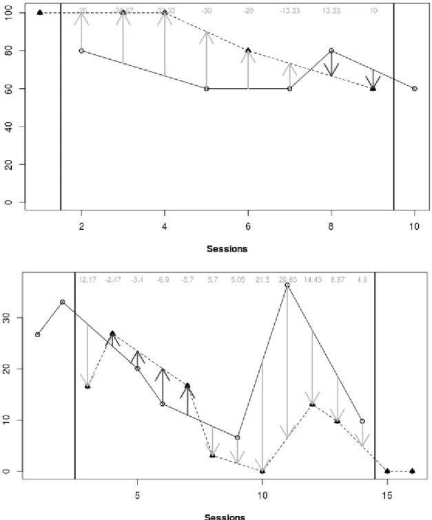
https://manolov.shinyapps.io/ATDesign/). The upper panel of Figure 1 shows two data paths
with five measurement occasions per condition, whereas the lower panel shows two data paths:
one condition takes place on seven measurements occasions and the other on nine. The
comparisons performed in VSC and ALIV are the ones marked with arrows, illustrating how
according to the number of consecutive administrations of the same condition, the number of
Figure 1. Comparison of data paths, illustrating the exclusion of first and last measurements. Upper panel: data by Yakubova and Bouck (2014), aim to increase the target behavior. Lower panel: data by Eilers and Hayes (2015), aim to decrease the target behavior.
ALIV computes the difference between the two data paths for each measurement occasion.
Afterwards, the average of these differences is computed. In order to obtain the statistical
significance of the outcome, ALIV is computed for all possible sequences that could have been
obtained at random. These ALIV values form the reference (randomization) distribution. The
actual outcome is located in the randomization distribution and the p value is the proportion of
ALIV values that are as large as or larger than the outcome. That is, a one-tailed test is
performed under the assumption that the researcher should know the direction of the difference
before carrying out the experiment (Levin et al., 2017).
VSC focuses on the same measurement occasions as ALIV. It counts the number of
occasions for which the condition B is superior (here greater) than the condition A. Afterwards,
this number is compared to a cut-off value presented by Lanovaz et al. (2017): if it is greater than
the cut-off value, it is concluded that there is evidence of the superiority of condition B. Lanovaz
et al. (2017) present cut-off values for VSC only for data series with equally represented
conditions, leading to even-number lengths (10, 12, 14, etc.), which is why we focus on the same
situations in the current text3.
The third means of comparison was based on the count obtained in VSC and the binomial
distribution. The probability of achieving as many successes or more in the number of
comparisons performed is obtained via the binomial distribution (the number of comparisons is
3 In the only supplementary material were all results are presented in tables (https://osf.io/yr8tg/), we also included results for ATD-RR and odd-number series lengths (11, 13, 15, etc.), for conditions unequally represented conditions. When deciding the cut-off values for VSC, we preferred a
conservative approach, using for each odd-number length n (11, 13, etc.) the cut-off value established for 𝑛 + 1 measurements (i.e., 12, 14, and so forth, respectively). However, given that such approach might be at odds with the intention to increase statistical power, the results are not commented here.
the number of trials and the probability of success at random is 0.5). If this binomial probability
is equal to or lower than .05, it is concluded that there is evidence of the superiority of condition
B. The inclusion of the binomial test was in order to check whether a simple solution to
obtaining p values, not requiring the use of VSC or ALIV, would prove to be appropriate.
Type I error rates were estimated as the proportion of p values (for ALIV and for the
binomial model) or the proportion of results above cut-off values (for VSC) out of all 1,000 iterations of conditions with absence of effect (𝛽2 = 0). For an adequate control of Type I error
rates, our intention was to use Serlin’s (2000) criterion for robustness, 𝛼 ± 25%𝛼, requiring
Type I error rates between 0.0375 and 0.0625, which is a in between Bradley’s (1978) stringent
and liberal criteria. Nevertheless, according to Robey and Barcikowski with 1,000 iterations, Bradley’s (1978) liberal criterion has to be followed, 𝛼 ± 50%𝛼, requiring proportions between
0.025 and 0.075. Statistical power is estimated as the same proportion but computed for
conditions with effect simulated (𝛽2 ≠ 0). Power is judged to be appropriate if it is at least 0.80,
following Cohen (1992).
Results
Type I Error Rates
Effect of the number of measurements for independent data. For both ATD-RR and ATD-RB the Type I error rates are controlled by VSC and ALIV+RT, regardless of the number
of measurements. (see the left panels of Figure 2). Actually, Type I error rates were controlled for all conditions tested (i.e., when 𝑛 ≥ 10). In contrast, the Type I error rates for the binomial
test were systematically greater than the upper limit of the liberal criterion, 0.075: the false alarm
Type I error rates with the number of measurements. Thus, it could be stated that the binomial
test applied to the number of comparisons for which the data path of one condition is superior to
the data path of the other condition is inappropriate even for independent data.
Effect of autocorrelation. The presence of autocorrelation does not seem to be related with systematic changes in the Type I error for either of the three tests (see the right panels of Figure
2 for an example). Thus the results commented for independent data are also applicable here.
The graphical illustrations provided focus on the shortest series length, but given that the effect
of the number of measurements is only slight, these illustrations provide an appropriate summary
Figure 2. A selection of results for Type I error rates for alternating treatments designs with restricted randomization (ATD-RR) and with randomized blocks (ATD-RB). Legend: black dotted line: ALIV plus randomization test; dark grey dashed line: binomial test; grey solid line: visual structured criterion (VSC)
Statistical Power
Effect of the number of measurements for independent data. As expected, statistical power increases with the number of measurements (see Figure 3). When 𝛽2 = 1, power never
reaches 0.8 for either of the tests and designs. When 𝛽2 = 2, a power of 0.8 is reached for all
three tests for ATD-RB already for 𝑛 = 12. Also for 𝛽2 = 2 and 𝑛 = 12, the ALIV+RT and the
binomial test reach power higher than 0.8. When 𝛽2 = 3, all three tests reach a power of 0.8 for
ATD-RB already for 𝑛 = 10. For ATD-RR, ALIV+RT and the binomial test reach this power
for 𝑛 = 10 and VSC for 𝑛 = 12.
In general, power is highest for the binomial test (which does not control for Type I error
rates), whereas it is lowest for VSC. For VSC, power is clearly lower for ATD-RR than for
Figure 3. A selection of results for statistical power as a function of the number of measurements; for alternating treatments designs with restricted randomization (ATD-RR) and with randomized blocks (ATD-RB). Legend: black dotted line: ALIV plus
Effect of autocorrelation. Positive autocorrelation is associated with higher statistical power (see Figures 4 and 5). Considering that positive autocorrelation does not lead to higher Type I
error rates, such conditions cannot be labelled as jeopardizing the performance of VSC and
ALIV+RT. In contrast, data with negative autocorrelation are unfavorable for these techniques.
However, the average corrected autocorrelation reported for ATDs by Shadish and Sullivan (2011) is approximately zero (−0.01).
Figure 4. A selection of results, for n=10, for statistical power as a function of the degree of autocorrelation; for alternating treatments designs with restricted randomization (ATD-RR) and with randomized blocks (ATD-RB). Legend: black dotted line: ALIV plus randomization test; dark grey dashed line: binomial test; grey solid line: visual structured criterion (VSC).
Figure 5. A selection of results, for n=20, for statistical power as a function of the degree of autocorrelation; for alternating treatments designs with restricted randomization (ATD-RR) and with randomized blocks (ATD-RB). Legend: black dotted line: ALIV plus randomization test; dark grey dashed line: binomial test; grey solid line: visual structured criterion (VSC).
Discussion
The present study provides initial simulation evidence on the performance of ALIV (Manolov &
Onghena, 2017) plus a randomization test and it provides further evidence on the performance of
VSC (Lanovaz et al., 2017) for ATD-RR and ATD-RB. Additionally, the study also extends the
evidence available on the performance of randomization tests with ATDs: (a) Levin et al. (2012)
studied systematically alternating designs (e.g., ABABABABABAB) with 12 and 24
measurement occasions; (b) Michiels et al. (2017) studied the conditional power (Keller, 2012)
for ATD-RR and ATD-RB with 12 to 40 measurement occasions; and both (a) and (b) used the
mean difference (not ALIV) as a test statistic. In what follows, we compare the current results
with these previous findings.
Lanovaz et al. (2017), focusing on systematic ATD found that VSC controlled the Type I error rate for 𝑛 ≥ 10. Additionally, Type I error rates decreased with autocorrelation (i.e., there
was a negative relation). Our findings for VSC applied to ATD-RR and ATD-RB, both with
random alternation of conditions, are consistent, in terms of Type I error rates being controlled.
Autocorrelation does not seem to have a clear positive or negative relation with false alarm rates. Statistical power reached 0.80 for 𝛽2 = 2, but not for 𝛽2 = 1; regardless of the number of
measurements. Power increased with autocorrelation. Our findings concur with the positive relation between power and autocorrelation, but for VSC a power of 0.80 for 𝛽2 = 2 is only
reached when there are 12 measurements in an ATD-RB and 16 measurements in an ATD-RR.
Thus, the current results concur with previous findings for systematic ATDs that the main
strength of VSC is ensuring that false alarm rates are controlled, whereas power may be
Levin et al. (2012) found that Type I error rate was controlled for the systematic ATD when
the autocorrelation was positive autocorrelation, whereas for ATD-RB it was always controlled.
Our findings for the randomization test using ALIV as test statistic show that the false alarm rate
is always controlled for both the ATD-RR and the ATD-RB. According to Levin et al. (2012), the statistical power for 𝛽2 = 2 and 𝑛 = 12, statistical power reached 0.8 for ATD-RB for
practically all degrees of autocorrelation tested and it was above 0.8 for the systematic ATD. Our findings for 𝛽2 = 2 and 𝑛 = 12 using ALIV as test statistic are practically identical to those
reported by Levin and colleagues (2012). Therefore, the correspondence between the current
findings and previous evidence is high and the conclusions about the performance of the
randomization test can be generalized beyond systematic ATDs and beyond the mean difference
as a test statistic.
Michiels et al. (2017) found that the conditional power for RR is higher than for
ATD-RB and our findings are consistent for ALIV as a test statistic. Moreover, despite some notable
differences between the two studies (i.e., test statistic, conditional vs. unconditional power
studied, two-sided vs. one-sided alternative hypothesis), both suggest that a medium-sized effect
(according to the benchmarks proposed by Harrington & Velicer, 2015) such as 2 standard
deviations can be detected as statistically significant with sufficient power for ATD-RR with as
few as 12 measurement occasions, whereas small effects such as 1 standard deviation require
more than 30 measurement occasions.
The current evidence suggests that VSC with the cut-off values derived for systematic alternation
(i.e., ABABABABAB) does not produce excessive false alarm rates even for ATD-RR and
RB. In terms of statistical power, we found that it was higher for RB than for
ATD-RR. We speculate that this finding might be related to the type of ATD for which the VSC were
developed (systematic) and the sequences that can be obtained in ATD-RB and ATD-RR. For a
systematic ATD, there is necessarily only one administration of the A or B conditions in the
beginning and in the end of the sequence (i.e., for n=10, ABABABABAB or BABABABABA).
For an ATD-RB, this is also the case; for instance, for n=10, a sequence such as
ABABBABAAB can be obtained, but the sequence AABABABABB cannot be obtained (but it
is possible under ATD-RR). Both the systematic sequence ABABABABAB and the randomized
block sequence ABABBABAAB (which is also acceptable in an ATD-RR) entail eight
comparisons, whereas the ATD-RR sequence AABABABABB would entail only six
comparisons. Therefore, for the same number of measurement occasions, for some random
sequences but not for all of them, the number of comparisons can be different. This could explain
the differences in power, given that when fewer comparisons are performed, the VSC requires a
greater percentage of superiority of one condition over the other in order to detect the presence of
an intervention effect. Therefore, applied researchers are encouraged to use VSC for either
systematic ATDs or ATD-RB.
Overall, the Type I error rates for ALIV plus a randomization test are closer to the nominal
value of .05 and this test also presents greater statistical power than the VSC. In order to be able
to use the inferential information, we recommend using randomization in the design, ALIV as a
descriptive measure of the difference between data paths and a randomization test for estimating
Regarding the usefulness of ALIV as a descriptive measure (i.e., an effect size in raw or
unstandardized terms), it is not subjected to presence of randomization in the design. Given that
a comparison between data paths is performed, ALIV is appropriate for ATDs, but not for
multiple-baseline designs or ABAB designs. In relation to adapted ATDs in which nonreversible
behaviors are studied, ALIV can be applied to part of the information obtained (e.g., the
percentage of steps executed correctly under two conditions compared), but it would not be
useful to quantify other critical aspects, such as the rapidity of learning, the extent of
maintenance and generalization, or the breath of learning (Wolery et al., 2014). Thus, we
encourage researchers to consider all pieces of evidence and we also echo recent calls for greater
prominence of social validity assessment (Snodgrass, Chung, Meadan, & Halle, 2018).
Regarding the inferential use of ALIV, the possibility to obtain a p value via a randomization
test applied to the ALIV outcome is not intended be a substitute for visual analysis. Moreover,
statistical significance should not be understood in terms of inference from an individual to a
population, but rather in relation to the null hypothesis of no differential effect of the intervention
(Edgington, 1967). We rather recommend that visual inspection be used together with
considering the descriptive value of ALIV and the p value. In that sense, we concur with
previous recommendations for the joint use of visual and statistical analysis (e.g., Franklin,
Gorman, Beasley, & Allison, 1996; Harrington & Velicer, 2015). If all pieces of evidence
coincide that there is a difference between the conditions, an inference of a causal effect of the
intervention on the target behavior would be justified in presence of a random determination of
the alternating sequence (Kratochwill & Levin, 2010).
The application of ALIV and the randomization test has been made feasible thanks to the
web application for ATD data analysis https://manolov.shinyapps.io/ATDesign/. In the newly
created tab, the statistical significance of ALIV can be obtained for ATD-RR and ATD-RB
having 3 or more measurement occasions per condition, although such data short series may be
deemed insufficient (Kratochwill et al., 2010; Wolery et al., 2014). Additionally, it should be
noted that the validity of the p values obtained is subjected to randomization actually being used
in the determination of the alternation sequence.
The p values obtained are the result of listing systematically all possible randomizations for
ATD-RR with up to 11 measurements per condition and for ATD-RB with up to 12
measurements per condition (i.e., the same cases studied in the present simulation). For longer
series, the p values are based on 1,000 randomly selected sequences, which are used for
constructing the randomization distribution. In that sense, for these longer series, the p value
obtained is not an exact p value, but a p value approximated by Monte Carlo sampling. Using
1,000 random samples for estimating the p value is well-aligned with previous research (Hayes,
1996; Levin et al., 2012; Michiels et al., 2017).
Implications for Methodologists
We consider that it is important that methodologists offer tools that could be potentially
attractive to applied researchers, apart from being methodologically sounds. In that sense, ATDs
offer a unique opportunity, given that randomization has been shown to be common in these
designs (Manolov & Onghena, 2017). Moreover, proposals such as VSC and ALIV are closely
related to the graphical representation of the data, which is the basis of visual analysis, because
design options (randomization in determining the condition for each measurement occasion) and
an empirically-tested quantification based on the data features object of visual analysis, another
relevant ingredient of a potentially attractive analytical procedure is a user-friendly free software.
However, it is yet to be verified whether these expected advantages of an analytical proposal
such as ALIV plus a randomization test are perceived as such by applied researchers.
Limitations and Future Research
The current paper only focuses on analytical procedures that compare data paths (i.e.,
combinations of actual and interpolated values). Other analytical options included comparing
only actually obtained measurements (e.g., Wolery et al., 2014) or comparing intercepts and
slopes, that is, only the estimates of the parameters of the models underlying the actual data
(Aerts, 2015).
In terms of the evidence provided here, the simulation conditions included data with no trends
and they can be expanded by including trends in the data paths. For instance, further
comparisons can be performed for crossing data paths (i.e., an upward trend in one condition,
starting from a lower initial level, and a downward trend in the other condition, starting from a
higher initial level) and for data paths that are increasing separated with each successive
measurement occasion (i.e., an upward trend in one condition, starting from a higher initial level,
and a downward trend in the other condition, starting from a lower initial level).
Moreover, the evidence provided in the current text is solely based on simulated data.
power, obtaining information regarding the former aspect is also possible using real data and
extended baselines (Lanovaz et al., 2017; Lanovaz, Huxley, & Dufour, 2017).
A different line of research can focus on studying the degree to which applied researchers are
open to incorporating p values in their assessment of the difference between conditions in an
ATD. They are likely to be fond of descriptive measures such as ALIV, considering the results of
the review (Manolov & Onghena, 2017) showing that most of the ATD published studies
References
Aerts, X. Q. (2015). Time series data analysis of single subject experimental designs using
Bayesian estimation. Doctoral dissertation. Retrieved November 13, 2017 from
https://digital.library.unt.edu/ark:/67531/metadc804882/m2/1/high_res_d/dissertation.pdf
Arnau, J., & Bono, R. (2004). Evaluating effects in short time series: Alternative models of
analysis. Perceptual and Motor Skills, 98, 419-432.
Barlow, D. H., & Hayes, S. C. (1979). Alternating treatments design: One strategy for comparing
the effects of two treatments in a single subject. Journal of Applied Behavior Analysis, 12,
199–210.
Barlow, D. H., Nock, M. K., & Hersen, M. (2009). Single case experimental designs: Strategies
for studying behavior change (3rd ed.). Boston, MA: Pearson.
Beretvas, S. N., & Chung, H. (2008). An evaluation of modified R2-change effect size indices
for single-subject experimental designs. Evidence-Based Communication Assessment and
Intervention, 2, 120-128.
Bradley, J. V. (1978). Robustness? British Journal of Mathematical and Statistical Psychology,
31, 144-152.
Bulté, I., & Onghena, P. (2013). The single-case data analysis package: Analysing single-case
Carriere, K. C., Li, Y., Mitchell, G., & Senior, H. (2015). Methodological considerations for
N-of-1 trials. In J. Nikles & G. Mitchell (Eds.), The essential guide to N-N-of-1 trials in health
(pp. 67-80). New York, NY: Springer.
Cohen, J. (1992). A power primer. Psychological Bulletin, 112, 155-159.
Edgington, E. S. (1967). Statistical inference from N=1 experiments. The Journal of Psychology,
65, 195–199.
Edgington, E. S., & Onghena, P. (2007). Randomization tests (4th ed.). London, UK: Chapman
& Hall/CRC.
Eilers, H. J., & Hayes, S. C. (2015). Exposure and response prevention therapy with cognitive
defusion exercises to reduce repetitive and restrictive behaviors displayed by children with
autism spectrum disorder. Research in Autism Spectrum Disorders, 19, 18–31.
Ferron, J. M., Foster-Johnson, L., & Kromrey, J. D. (2003). The functioning of single-case
randomization tests with and without random assignment. The Journal of Experimental
Education, 71, 267-288.
Ferron, J. M., Moeyaert, M., Van den Noortgate, W., & Beretvas, S. N. (2014). Estimating
causal effects from multiple-baseline studies: Implications for design and analysis.
Psychological Methods, 19, 493-510.
Ferron, J. M., & Ware, W. (1995). Analyzing single-case data: The power of randomization tests.
Franklin, R. D., Gorman, B. S., Beasley, T. M., & Allison, D. B. (1996). Graphical display and
visual analysis. In R. D. Franklin, D. B. Allison, & B. S. Gorman (Eds.), Design and analysis
of single-case research (pp. 119–158). Mahwah, NJ: Erlbaum.
Harrington, M., & Velicer, W. F. (2015). Comparing visual and statistical analysis in single-case
studies using published studies. Multivariate Behavioral Research, 50, 162–183.
Hayes, A. F. (1996). Permutation test is not distribution-free: Testing H0: ρ = 0. Psychological
Methods, 1, 184-198.
Heyvaert, M., & Onghena, P. (2014). Randomization tests for single-case experiments: State of
the art, state of the science, and state of the application. Journal of Contextual Behavioral
Science, 3, 51–64.
Huitema, B. E., & McKean, J. W. (2000). Design specification issues in time-series intervention
models. Educational and Psychological Measurement, 60, 38-58.
Keller, B. S. (2012). Detecting treatment effects with small samples: The power of some tests
under the randomization model. Psychometrika, 77, 324-338.
Kratochwill, T. R., Hitchcock, J. H., Horner, R. H., Levin, J. R., Odom, S. L., Rindskopf, D. M.,
& Shadish, W. R. (2013). Single-case intervention research design standards. Remedial and
Special Education, 34, 26-38.
Kratochwill, T. R., & Levin, J. R. (2010). Enhancing the scientific credibility of single-case
Lanovaz, M., Cardinal, P., & Francis, M. (2017, November 2). Using a visual structured criterion
for the analysis of alternating-treatment designs. Behavior Modification. Advance online
publication. https://doi.org/10.1177/0145445517739278
Lanovaz, M. J., Huxley, S. C., & Dufour, M. M. (2017). Using the dual‐criteria methods to
supplement visual inspection: An analysis of nonsimulated data. Journal of Applied Behavior
Analysis, 50, 662-667.
Ledford, J. R., Lane, J. D., & Severini, K. E. (2018). Systematic use of visual analysis for
assessing outcomes in single case design studies. Brain Impairment, 19, 4-17.
Levin, J. R., Ferron, J. M., & Gafurov, B. S. (2017). Additional comparisons of
randomization-test procedures for single-case multiple-baseline designs: Alternative effect types. Journal of
School Psychology, 63, 13-34.
Levin, J. R., Ferron, J. M., & Kratochwill, T. R. (2012). Nonparametric statistical tests for
single-case systematic and randomized ABAB…AB and alternating treatment intervention
designs: New developments, new directions. Journal of School Psychology, 50, 599-624.
Levin, J. R., Lall, V. F., & Kratochwill, T. R. (2011). Extensions of a versatile randomization test
for assessing single-case intervention effects. Journal of School Psychology, 49, 55-79.
Manolov, R., & Onghena, P. (2017, March 16). Analyzing data from single-case alternating
treatments designs. Psychological Methods. Advance online publication.
http://dx.doi.org/10.1037/met0000133
Michiels, B., Heyvaert, M., & Onghena, P. (2017, April 7). The conditional power of
A Monte Carlo simulation study. Behavior Research Methods. Advance online publication.
doi: http://dx.doi.org/10.3758/s13428-017-0885-7
Moeyaert, M., Ugille, M., Ferron, J., Beretvas, S. N., & Van Den Noortgate, W. (2014). The
influence of the design matrix on treatment effect estimates in the quantitative analyses of
single-case experimental designs research. Behavior Modification, 38, 665–704.
Onghena, P., & Edgington, E. S. (1994). Randomization tests for restricted alternating treatments
designs. Behaviour Research and Therapy, 32, 783–786.
Onghena, P., & Edgington, E. S. (2005). Customization of pain treatments: Single-case design
and analysis. Clinical Journal of Pain, 21, 56–68.
Onghena, P., & Van Damme, G. (1994). SCRT 1.1: Single-case randomization tests. Behavior
Research Methods, Instruments, & Computers, 26, 369.
Robey, R. R., & Barcikowski, R. S. (1992). Type I error and the number of iterations in Monte
Carlo studies of robustness. British Journal of Mathematical and Statistical Psychology, 45,
283-288.
Serlin, R. C. (2000). Testing for robustness in Monte Carlo studies. Psychological Methods, 5,
230-240.
Shadish, W. R., & Sullivan, K. J. (2011). Characteristics of single-case designs used to assess
intervention effects in 2008. Behavior Research Methods, 43, 971–980.
Smith, J. D. (2012). Single-case experimental designs: A systematic review of published research
Snodgrass, M. R., Chung, M. Y., Meadan, H., & Halle, J. W. (2018). Social validity in
single-case research: A systematic literature review of prevalence and application. Research in
Developmental Disabilities, 74, 160-173.
Solmi, F., Onghena, P., Salmaso, L., & Bulté, I. (2014). A permutation solution to test for
treatment effects in alternation design single-case experiments. Communications in Statistics
- Simulation and Computation, 43, 1094–1111.
Wolery, M., Gast, D. L., & Ledford, D. (2014). Comparison designs. In D. L. Gast & J. R.
Ledford (Ed.), Single subject research methodology in behavioral sciences: Applications in
special education and behavioral sciences (pp. 297-345). London, UK: Routledge.
Yakubova, G., & Bouck, E. C. (2014). Not all created equally: Exploring calculator use by
students with mild intellectual disability. Education and Training in Autism and