Università Politecnica delle Marche
Scuola di Dottorato di Ricerca in Scienze dell’Ingegneria Curriculum in Ingegneria Informatica, Gestionale e dell’ Automazione
Kinematic Control Algorithms for
Cooperative Dual-arm Systems via
Redundancy Resolution
Ph.D. Dissertation of:
dott. Davide Ortenzi
Advisor:
Chiar.mo Prof. Sauro Longhi
Coadvisor:
dott. Andrea Monteriù dott. Alessandro Freddi
Curriculum Supervisor:
Università Politecnica delle Marche
Scuola di Dottorato di Ricerca in Scienze dell’Ingegneria Facoltà di Ingegneria
"Fatti non foste a viver come bruti,
ma per seguir virtute e canoscenza”
Divina Commedia,
Dante Alighieri.
Acknowledgments
The present study has been supported by several people, who have helped to improve important skills.
First of all, I would thank my tutor, Prof. Sauro Longhi, for giving me the opportunity to carry out my research also at a prestigious foreign university, such as Aalto University of Helsinky.
Moreover, all my results obtained during the research activity have been made possible thanks to two fundamental people as my supervisors: Andrea and Alessandro. I would like to thank them for all their precious and tireless help for everything, especially during the writing of our publications, many of which completed together late at night. However, the most important thing that I received from their research activities concerns the passion for this work, which often requires a lot of sacrifice and motivation.
I would thank Prof. Ville Kyrki, who welcomed me into his research group and supported my research during my visiting time in Finland. From this ex-perience, I have learned the organization and methodology that he has always demonstrated in his work. Moreover, I would thank Raj, with whom I pleas-antly collaborated and all the colleagues in the office, as Mattia and Roel, who made my period in Finland really pleasant.
A great thank to Patrizia and her talent, because her illustrations help to clarify the basic concepts of my research topics.
I thank my colleagues of department, which have become also my friends. They have always supported me, with their professional experience in order to improve the quality of my research activity, especially at the beginning of this PhD course. I think that my research results would not be so pleasant, without the enthusiasm of (in alphabetic order) Francesco, Giovanni, both Luca, Lucia, Lucio, Luigi and Sabrina.
For last one, but most important one, I thank my girlfriend Chiara, because, in spite of the big distance that separates us, she still continues to support me tirelessly in all my changes, of today and tomorrow...
Ancona, Marzo 2017
Abstract
This thesis tackles the problem of kinematic control for cooperative dual-arm systems via redundancy resolution. First the redundancy analysis of two co-operative manipulators is presented, which shows how they can be considered as a single redundant manipulator, through the use of the relative Jacobian matrix. Then the Jacobian null space technique is considered: in this way the kinematic redundancy can be resolved by applying the principal local optimiza-tion techniques used for the single manipulator case; moreover several tasks with different execution priority levels can be performed at the same time (e.g. obstacle avoidance, manipulability index maximization or joint position con-straints satisfaction). The kinematic resolution is then specifically addressed to both prevent and take into account possible faults. In detail, since violation of joint position constraints may damage a manipulator, a joint position limit avoidance strategy is proposed. This strategy is able to satisfy all joint limits even when the number of redundant motions are no longer sufficient to ensure them with a classical approach, by locally and temporary changing the desired end-effectors motion when redundant motions are not available. Finally, a fault tolerance algorithm is proposed, which use the degree of redundancy both to maximize the local optimum fault tolerance configuration, and to overcome the loss of the end effector velocity due to fault occurrence, by use of the sat-uration null space method. Several simulated and experimental examples are illustrated, which demonstrate the high flexibility of the proposed algorithms, which can implemented on different kind of cooperative manipulators.
Sommario
Questa tesi affronta il problema del controllo cinematico di due manipolatori cooperanti, attraverso la risoluzione della ridondanza cinematica. In primo lu-ogo, la tesi propone una descrizione dell’analisi della ridondanza dovuta alla cooperazione dei manipolatori, poichè essi possono essere considerati come un unico manipolatore ridondante, mediante il metodo dello Jacobiano rela-tivo. Successivamente, viene studiata la tecnica di risoluzione della ridondanza basata sulla proiezione di diversi compiti nello spazio nullo dello Jacobian, in modo da eseguire contemporaneamente diversi compiti, aventi differenti livelli di priorità. Tali compiti possono migliorare la cooperazione dei due manipo-latori, come ad esempio, evitare gli ostacoli posti in prossimità, massimizzare l’indice di manipolabilità o rispettare i vincoli di posizione presenti nei giunti. In particolare, la violazione di vincoli di posizione dei giunti è dettagliatamente studiata, poichè tale condizione può indurre a molteplici criticità, fra le quali il danneggiamento del sistema stesso. Pertanto, é proposta una strategia di controllo che permette di rispettare tutti i limiti dei giunti, anche qualora il numero di movimenti ridondanti non fosse più sufficiente a garantirli mediante un approccio classico. Tale tecnica degrada, parzialmente e temporaneamente, le prestazioni del movimento assegnato ai due terminali, al fine di rispettare tutti i vincoli di giunto, anche quando i moti ridondanti non sono disponibili. Infine, viene proposto un algoritmo di tolleranza del guasto, che impiega il grado di ridondanza del sistema sia per ottimizzare localmente una configu-razione dei manipolatori robusta al guasto, che per limitarne i suoi effetti sulle loro prestazioni. Alcuni esempi di possibili applicazioni sono stati realizzati sia in simulazione che sperimentalmente. Essi dimostrano l’elevata flessibilità degli algoritmi proposti che possono essere adeguatamente implementati su diverse tipologie di manipolatori.
Contents
1 Introduction 1 1.1 Motivations . . . 1 1.2 Literature review . . . 3 1.3 Contributions . . . 5 1.4 Thesis structure . . . 52 Kinematic redundant manipulators 7 2.1 Manipulator mobility . . . 7 2.2 Spaces definition . . . 9 2.2.1 Joint space . . . 9 2.2.2 Cartesian space . . . 9 2.2.3 Workspace . . . 10 2.2.4 Task space . . . 10
2.3 Kinematic redundancy definition . . . 10
2.4 Differential kinematics . . . 12
2.4.1 Geometric Jacobian . . . 13
2.4.2 Analytical Jacobian . . . 15
2.4.3 Inverse differential kinematics . . . 17
3 Redundancy resolution via local optimization 21 3.1 Jacobian pseudo-inverse method . . . 21
3.2 Jacobian null space method . . . 24
3.2.1 Jacobian null space projection matrix . . . 24
3.2.2 Gradient projection method . . . 26
3.2.3 Objective functions . . . 27
3.2.4 Saturation in the null space method . . . 27
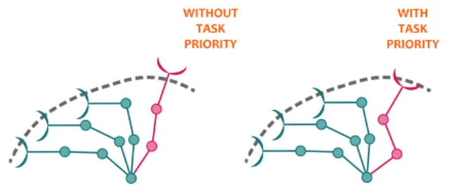
3.2.5 Hierarchical priority execution task . . . 29
4 Kinematic modelling of cooperative manipulators 33 4.1 Relative Jacobian method . . . 33
Contents
5 Proposed kinematic control algorithms for obstacle and joint limits
avoidance 39
5.1 Control algorithm for obstacle avoidance . . . 39
5.1.1 Case study . . . 39
5.1.2 Task Description . . . 39
5.1.3 Simulation results . . . 43
5.2 Control algorithm for joint limits avoidance . . . 46
5.2.1 Proposed joint position limits avoidance strategy . . . . 47
5.2.2 First case study . . . 49
5.2.3 Second study case . . . 53
5.2.4 Supervisor controller for redundancy management . . . 58
5.2.5 Third study case . . . 60
6 Proposed fault tolerant algorithms 65 6.1 Relative manipulability index . . . 65
6.2 Optimization of fault tolerant configuration . . . 67
6.3 Proposed fault tolerant configuration algorithm . . . 68
6.4 Joint fault management with the SNS method . . . 69
6.5 Case study . . . 70
6.5.1 Results . . . 71
6.5.2 Discussion . . . 73
7 Conclusions and future works 75 7.1 Conclusions . . . 75
7.2 Future works . . . 76
List of Figures
2.1 Three-link planar arm (revised version of Figure 2.20 from [55]) 8 2.2 Calculation of i−th joint velocity contribution to the end-effector
velocity (revised version of Figure 3.2 from [55]) . . . 14
2.3 Block diagram of the close loop inverse kinematics (partial re-production of Figure 3.11 from [55]) . . . 18
3.1 Example of non-repeatable motion in the joint space . . . 23
3.2 Relation between joint velocity space and end-effector velocity space . . . 24
3.3 Geometric view on Jacobian null space . . . 25
3.4 Example of SNS application . . . 29
3.5 Example of hierarchical priority execution task . . . 30
4.1 Two cooperative manipulators (partial reproduction of Figure 1 from [26]) . . . 34
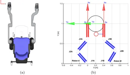
4.2 Block diagram of the relative Jacobian pseudo-inverse algorithm 37 5.1 Concept of the wheelchair with two manipulators within an AAL scenario . . . 40
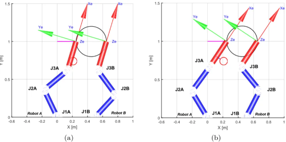
5.2 Top view of the system (a) and initial planar manipulators con-figuration (b) . . . 40
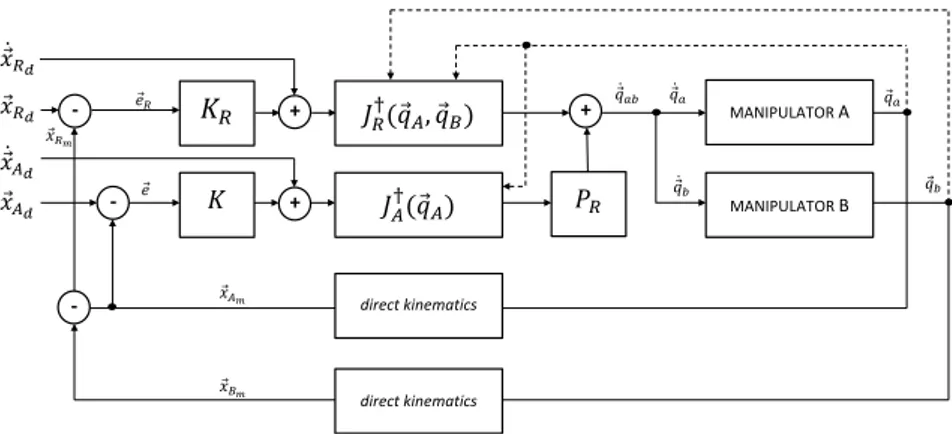
5.3 Block diagram of two cooperative manipulators . . . 43
5.4 Final manipulators configuration without (a) and with (b) ob-stacle avoidance task. . . 44
5.5 Joint angle position without (a) and with (b) obstacle avoidance task . . . 44
5.6 Relative end-effectors position error (a) and orientation error (b) 45 5.7 End-effector A position along the path (a) and the path following error (b) . . . 45
5.8 Minimum distance between manipulators and obstacle . . . 46
5.9 Activation function for one component wi of W matrix. . . . . 48
5.10 Operating principle of the joint limits avoidance strategy. . . . 49
5.11 Manipulator configurations: (a) initial, (b) Case I and III final configuration, (c) Case II final configuration.) . . . 50
List of Figures
5.12 A (B) manipulator joint position space relative to qA1-qA2 (a)
(qB1-qB2 (b)). . . 52
5.13 A and B manipulators Cartesian path for the three considered simulation cases. . . 53
5.14 Joint velocity space with repulsive velocity for A manipulator and B manipulator. . . . 54
5.15 Two robot manipulators holding a woodblock to perform tightly coordinated cooperative operations. . . 55
5.16 Heterogeneous two-robot system: coordinate frame transforma-tion for the relative Jacobian formulatransforma-tion. . . 55
5.17 Coordinated manipulation results of tightly-coupled manipula-tors under joint constraints (Case B and C). . . 56
5.18 Cooperative performance of tightly-coupled manipulators for the Cases (Case A-C), refer to Table5.3. . . 57
5.19 Controller treats joint limits enforced in manipulators. . . 58
5.20 Operating principle of the supervisor controller. . . 59
5.21 Operating principle of the joints avoidance strategy. . . 60
5.22 Study case setup (a) and coordinate transformation of the Bax-ter arms (b) . . . 61
5.23 Controller treats joint limits enforced in manipulators. . . 63
5.24 Coordinated manipulation results. . . 63
5.25 Cooperative performance of tightly-coupled manipulators. . . . 64
6.1 3 DoF planar manipulator with fault tolerant configuration with respect to joint one (q1) (revised version of Figure 2 from [52]) 66 6.2 Starting configuration of the dual arm system . . . 70
6.3 Relative manipulability indices for 50% reduction of maximum joint velocity . . . 71
6.4 Relative manipulability indices for 80% reduction of maximum joint velocity . . . 71
6.5 Joint velocity when the maximum ˙q1 velocity is reduced of 50% at t=5s . . . 72
6.6 Joint velocity when the maximum ˙q3 velocity is reduced of 50% at t=5s . . . 72
6.7 Final manipulators configuration, when a 80% maximum veloc-ity loss on (a) ˙q1and (b) ˙q3 occurs at t=5s . . . 73
List of Tables
5.1 Joint limits. . . 50
5.2 Decomposition of the task into prioritized subtasks. . . 51
5.3 Experimental cases. . . 53
5.4 Joint limit parameters. . . 56
5.5 Description of the experimental considered cases. . . 62
Chapter 1
Introduction
Dual-arm manipulation systems have been attracting a growing from the sci-entific community over the last few years. Although a universal accepted def-inition does not exist, a good starting point is provided [1], where dual arm manipulation is presented as the cooperation of two robotic systems physi-cally interacting with an object, moving or reshaping it. The use of multiple cooperative manipulators offers several advantages in many different contexts [2]. Potential applications for cooperative manipulation include, but are not limited to, the manufacturing industry [3, 4, 5], hazardous environments such as nuclear sites [6, 7, 8], underwater [9, 10] and space [11, 12]. Cooperation can bring economical benefits since a wide range of tasks can be accomplished through the use of multiple simpler and less expensive heterogeneous robots [13].
The dual-arm manipulation system was firstly introduced to replace workers in dangerous manufacturing processes. Early robotic manipulators were con-structed by Goertz in the 1940s for handling radioactive goods [14]. Later, they were employed for marine and space exploration, where the dual arm manipu-lators were noticeably improved. In 1969, the NASA’s Johnson Space Center introduced anthropomorphic dual arm teleoperators, due to the analogies with human operations [15].
Today, the modern technological progress and the increasing acceptance of technology by users have encouraged the scientific community to focus on the development of dual-arm manipulators able to work in user centered envi-ronments, such as surgery[16] and Ambient Assisted Living (AAL) applica-tions [17]. An example of AAL application consists in dual-arm manipulators mounted on a wheelchair, which can assist disabled people to reach and handle objects, or to perform more complex tasks [18, 19, 20].
1.1 Motivations
Cooperation between two robotic arms manipulating an object is a challeng-ing task from an engineerchalleng-ing perspective, since their relative motions have to
Chapter 1 Introduction
be properly controlled in order to perform the desired operations. Moreover, the two arms and the object realize a closed kinematic where the degrees of motion of the system are greater than those which are generally required to perform the task, therefore the inverse kinematics problem admits an infinite number of solutions [21]. For this reason the dual-arm manipulation context, the redundant variables can be employed to perform tasks, such as collision avoidance [22], or satisfy specific performance criteria, such as singularities avoidance [23], mechanical joint limits avoidance [24] or improvement of ma-nipulability along a chosen direction [25]. Since the control of cooperative manipulators is more complex than the control of a single manipulator, I de-cided to employ a method based on the relative Jacobian matrix. This method permits to consider two redundant manipulators like a unique redundant ma-nipulator, whose number of joints is equal to the sum of each manipulator’s joints, while the end-effector motion variables correspond to the relative mo-tion between the two end-effectors. This method presents several advantages with respect to the individual control of each manipulator. Firstly, a dual-arm system modelled according to the relative Jacobian method can be controlled by the same algorithms used for controlling single manipulators. Secondly, the compact expression of the relative Jacobian matrix [26] is simple to calculate when Jacobians of the individual manipulators are known and, if a manipula-tor is replaced with another one, it is sufficient to change its Jacobian without the need of complex calculus. Therefore the research activity presented in this thesis is focused on this method. In particular the main objective of this the-sis is to extend the classical redundancy resolution algorithms for controlling dual-arm system, composed by homogeneous and heterogeneous manipulators. Moreover, since some cooperative dual-arm manipulators have been designed to perform tasks in harsh environments, they have to complete an assigned task even in presence of faults. In such a scenario, a dual-arm system can be defined as fault tolerant [27]. There are several sources of faults that can compromise the correct motion of manipulators. The main faults can be classified into five categories: Free-Swinging Joint Faults (FSJFs) [28], Locked Joint Faults (LJFs) or joint failure [29], Partial Loss of Joint Torque Faults (PLJTFs) [30], incorrectly measured Joint Position Faults (JPFs) and incorrectly measured Joint Velocity Faults (JVFs) [31]. The first three categories consist in a partial or total loss of joints motion, while the other two comprises joint sensors faults. The probability of occurrence of one of these faults on a robot is inversely related to the reliability of its components [32]. For this reason, a first fault tolerant approach consists in using high quality components, i.e. perfectness [33], which dramatically increase the system cost. Regarding to the PLJTFs, a low-cost fault tolerant system is proposed in this thesis. The basic idea consists of designing a kinematic controller based on redundancy resolution algorithm, 2
1.2 Literature review which allows both to maximizes the local optimum fault tolerance configuration (before joint fault) and to overcome the loss of the end effector velocity due to fault occurrence (after joint fault).
1.2 Literature review
Although only a few works focused on inverse kinematic control of dual arms motion, such problem has been addressed extensively in literature for the sin-gle manipulator case. The related research is mainly based on global and local optimization of a specific objective function. In particular, the global opti-mization permits to calculate the optimal path which satisfies a performance criteria (off-line mode) [34], like avoiding obstacles whose positions are known a priori, while the local optimization permits to calculate the current desired joints velocity in order to locally satisfy the performance criteria (real time
mode) [35].
The simplest local optimization technique is represented by the pseudo-inverse solution [36], which provides the joint velocity with the minimum norm among those satisfying the task constraint. This techniques do not permit to use the redundant joints for any secondary task, which is instead possible by adopting the so called task augmentation method [37]. The task augmentation method consists in augmenting the task vector to tackle additional objectives by implementing two different methods: extended Jacobian [38, 39] and aug-mented Jacobian [40]. The disadvantage of these two techniques is due to occurrence of singularities when the Jacobians associated with the additional objectives are linearly dependant [38, 41]. In order to overcome these problems, the Jacobian null space technique was proposed in [42]. This method consists of projecting a specific objective function (secondary task) into the Jacobian null space of another task with higher execution priority, in order to obtain a hierar-chical task priority structure, as described in [43, 44]. Since the joint velocities required by secondary tasks generate self-motions in the robot (changing the current manipulator configuration), they do not affect the performance of the task with highest priority, namely primary task.
A widely used technique of Jacobian null space is the Gradient Projection Method (GPM), which projects the gradient of a specific objective function in the null space of Jacobian associated with the desired task, in order to maximize/minimize it. The main drawback of GPM is the redundant motion needed to optimize the objective function (e.g. in the joint limits avoidance task, all joint positions are kept close to the mid-range joint position). In order to limit the number of redundant motions, other approaches operate only on those joints whose positions are close to the respective limits [45]. A recent work [46] projects a joint limit avoidance function based on Prescribed Performance
Chapter 1 Introduction
Control methodology (PPC) into the Jacobian null space of the desired task. However, since the dimension of the Jacobian null space depends on the number of the available redundant motions, PPC generally does not guarantee the execution of the secondary task. On the other hand, some algorithms based on Jacobian null space method ensure this execution by degrading the performance of primary task. One of these algorithms is described in [47] and consists of the division of the main task into several subtasks. Single subtasks can be removed and recovered by a supervisor controller in order to ensure a sufficient number of redundant motion to the secondary task. A different algorithm is the Saturation in the Null Space (SNS) algorithm [48], which considers the joint velocity limits avoidance as secondary task. In particular, this technique projects the exceeded joint velocity into the null space of the main task Jacobian matrix, namely partial Jacobian matrix, composed by the not-saturated joints velocity. When there are not sufficient redundant motions to guarantee the joint velocity constraints, the desired primary task velocity is reduced. Recently this algorithm was applied in the context of two cooperative manipulators affected by joint constraints [49]. The study involves the cooperation of two KUKA lightweight manipulators based on relative Jacobian method.
Focusing on the joint fault tolerance study, several method can be considered in the literature. In particular, a widely applied method consists in transform-ing a FSJF into a LJF, so that they are managed in the same way [50, 51], while the PLJTFs is kinematically modelled as a reduction of the maximum joints velocity due to a partial torque loss of its servomotor [30]. An efficient approach to compensate these types of faults in the end effector consists in the use of redundant degrees.
The manipulators’ configuration during a fault is crucial in fault tolerant applications. In fact, the degradation of the system performances depends on which joint of the manipulators is affected by the fault [51]. If the joint that provides the greater contribution to the end effector motion is faulty, then the performance will heavily drop. A classical example is the human arm which has to execute the task “drink”. It is clearly a redundant system because it has 7 DoF, but it is not fault tolerant respect to an elbow joint failure, since it is the only joint that can reduce the distance between the shoulder and the wrist. These critical configurations can be avoided by projecting the gradient of a suitable objective function into the Jacobian null space, in order to avoid bad joint positions before a fault/failure occurs [34]. Another approach is to maximize the manipulability index by calculating a proper objective function [25]. This method allows to obtain a local optimum configuration, because it involves a minimal reduction of the manipulability index for any joint failure. A possible way to know the amount of manipulability after a failure is to compute the relative manipulability index [52] which is the ratio between the 4
1.3 Contributions manipulability index after and before a failure. The research activity of this thesis about the fault tolerant applications is based on this last approach.
1.3 Contributions
Although several works focusing on the motion constraints and fault tolerant applications have been performed by several redundancy resolution algorithms in single manipulator case, only few works considered them in a cooperative manipulation scenario. Therefore the proposed research activity allowed to con-sider such methods for cooperative manipulators by using the relative Jacobian method.
Therefore, the research activity described in this thesis have led the following innovative contributions with respect to the state of the art:
• Implementation of the hierarchical execution task architecture based on relative Jacobian method [53];
• Analysis and development of a kinematic controller that provides coordi-nated motions and joint limit avoidance during the cooperation between a redundant and non-redundant manipulators;
• Development of a novel joint position limits avoidance strategy, which is able to satisfy all joint limits of homogeneous redundant manipulators, even when there are not available redundant motions;
• Development of a joint fault tolerance algorithm, which is able to guar-antee the correct cooperation of two planar manipulators when the max-imum velocity of a joint is reduced [54].
1.4 Thesis structure
The thesis has the following structure: Chapter II presents the knowledge about the kinematic redundancy with the introduction of the inverse differen-tial kinematics problem; Chapter III summarizes the theoretical background about the redundancy resolution algorithm that are subsequently used in the proposed kinematic controller. The derivation of the compact relative Jaco-bian formulation and its implementation in the kinematic control is proposed in Chapter IV, while the proposed algorithms with respect to the motion con-straints cases are described in Chapter V. Chapter VI describes the proposed fault tolerance algorithm, which has been tested on two planar cooperative manipulators. Conclusions and future works complete the thesis in Chapter VII.
Chapter 2
Kinematic redundant manipulators
This chapter focuses on some fundamental definitions necessary to well un-derstand the kinematic redundancy problem in the cooperative manipulation control framework.2.1 Manipulator mobility
The kinematically redundant manipulators are particular mechanical structures that possess more motion variables then those required to perform the specific task. This requires to first it is firstly necessary to analyse the manipulator mobility.
In robotics, the number of independent variables necessary to determine completely the system configuration in space is defined as Degrees of Freedom DoFs (or Degrees of Motion DoMs). This definition is different from that used to describe the pose of a rigid body (space’s DoF) in a space n-dimensional, by means of independent coordinates. In order to calculate the DoFs of a generic mechanism, namely F , it is possible to implement the formula in (2.1), which depends on several kinematic parameters:
F = λ(j − 1) −
n
∑
i=1
ci (2.1)
where ci is the imposed kinematic constraints of the i − th joint, n and j are
the number of joints and rigid links possessed by the mechanism (base link enclosed), while λ is the number of space’s DoFs.
Since for each joint, the sum of the number of constraints ci and permitted
degree of freedom fi have to be equal to the space’s DoF (λ = ci+ fi), it is
possible to obtain the total number of system constraints as:
n ∑ i=1 ci= n ∑ i=1 (λ − fi) = jλ − n ∑ i=1 fi (2.2)
Chapter 2 Kinematic redundant manipulators
𝑝�
𝑝�
𝑦₀
𝑦
𝑦₁
𝑦₂
𝑦₃
𝑥₀
𝑥
𝑥₁
𝑥₂
𝑥₃
𝑃
𝑞�
𝑞�
𝑞�
𝛼�
𝛼�
𝛼�
Figure 2.1: Three-link planar arm (revised version of Figure 2.20 from [55])
Grubler formula (when λ = 3):
F = λ(j − n − 1) +
n
∑
i=1
fi (2.3)
A possible application about (2.3) is to calculate the DoF of the planar manipulator shown in Figure 2.1 in accordance with Grubler formulation
The planar manipulator in Figure 2.1 is composed by j = 3 links and n = 3 joints placed on a planar space (λ = 3). Since all joints are rotative, they allow only the relative rotation between two consecutive links fi = 1, but not their
relative translation ci = 2, so that the manipulator DoFs is equals to three,
F = 3.
This result implies an important property about the mobility of manipulators having open-chain structure. In fact, for open chain manipulators, the DoFs are equal to the number of joints n (F = n), hence in the following chapters the DoF of a manipulator will be implicitly expressed by its number of joints
n.
2.2 Spaces definition A system composed by two planar cooperative manipulators having the same structure shown in Figure 2.1 has a DoF equals to six, (F = 2∗n = 6). However when they cooperate on a same object, a closed chain is realized and the DoF is smaller then the total number of joints, F < n. A possible demonstration can be given by applying (2.3) for a specific cooperation, in which the two end-effectors can change their relative orientation but not their relative positions. This type of cooperation can be kinematically modelled as a revolute joint belonging to the closed chain.
Therefore, the obtained structure has n = 7 but its DoF is equal to four, because 3 joint positions (passive joints) depend on the other 4 joints (active joints). Therefore, it is possible to assert that the loss of DoFs obtained during the cooperation depends on the number of kinematic constraints that are intro-duced from it. The motion of two cooperative manipulators will be examined in details in chapter 4.
2.2 Spaces definition
2.2.1 Joint space
The joint space (also called the configuration space) denotes the the space in which the n-dimensional vector of joint variables, q, is defined as [55]:
⃗ q = ⎡ ⎢ ⎢ ⎢ ⎢ ⎣ q1 q2 .. . qn ⎤ ⎥ ⎥ ⎥ ⎥ ⎦ (2.4)
where the i-th component qiof the vector q corresponds to the angular position
of i-th joint θi, qi= θi. Since the dimension of q is equal to the total number
of joints that are present in the structure, it is also equal to the DoFs of a open chair manipulator as discussed in the previous section. The joint space allows to obtain a unique description of the current configuration assumed by a manipulator and thus of its end effector pose via direct kinematics calculation.
2.2.2 Cartesian space
The Cartesian space is the space in which is defined the m-dimensional vector
xe(with m ≤ 6), in which are reported the variables that describe the position and the orientation of the end-effector [55]:
⃗ xe= [ ⃗ pe ⃗ φe ] (2.5)
Chapter 2 Kinematic redundant manipulators
where ⃗pe and ⃗φeindicate the Cartesian coordinate and minimum orientation representation (i.e. Euler angles) of the end-effector respect to the base frame. The Cartesian space is very useful for trajectory planning (path and execu-tion time) in the space, because the task variables are defined in this space, rather than joint space. However the end effector pose expressed in Carte-sian space depends on joint positions (Joint space) via the direct kinematics relation, which can be expressed as
⃗
xe= ⃗k(⃗q) (2.6)
where the vectorial function ⃗k, which is generally not linear, allows to calculate
the end effector pose in Cartesian space from the knowledge of joints position.
2.2.3 Workspace
When the joints position are varied across their entire operational range, the origin of the end-effector frame [55] describes a points region on the Cartesian space, which is called the workspace. Generally the workspace can be classified in reachable space and dexterous space. The latter defines the points region that the origin of the end effector frame can reach by several orientations, while the former is the region that the end effector frame can reach by at least orientation. Therefore the reachable space coincides with workspace, while the dexterous space is a subset of the previous one.
The workspace of a single manipulator depends on its geometry and joint position limits. However when two cooperative manipulators makes a closed kinematic chain the workspace is smaller than without cooperation, because it also depends on the type of cooperation and the distance between two manip-ulator bases.
2.2.4 Task space
The task space is the space in which is defined a r-dimensional vector ⃗xr, that is composed by the variables that are necessary to describe the end effector pose in order to perform the desired task [55]. The maximum number of variables is equal to the number of the Cartesian space variables (r ≤ m). This definition is very important to determine when a manipulator is redundant, as described in the next section.
2.3 Kinematic redundancy definition
Given the previous definitions, it is now possible to define formally the kine-matic redundancy of a robotic manipulator, as well as defined in [55].
2.3 Kinematic redundancy definition
Kinematic Redundancy A open-chain manipulator is kinematically redundant
when the number of DoFs n is greater than the number of variables r that are necessary to describe a given task (dimension of the task space),
n ≥ r.
Intrinsic Redundancy A manipulator is defined as intrinsically redundant when
the number of DoFs n is greater than the number of variables m relative to the Cartesian space in which the manipulator operates, n > m.
Functional Redundancy A manipulator is functionally redundant when the
number of DoFs n is equal to the dimension of the Cartesian space m (n = m), but the dimension of task space r is smaller than that of the Cartesian Space m, (from which it follows n > r).
The first is the main definition of redundancy, which demonstrates the de-pendence of the redundancy on the dimension of the specific task. Therefore the same manipulator can be redundant with respect to a specific task and non-redundant with respect to another task. This definition can be classified in two sub-categories: intrinsic and functional redundancy. In detail, the in-trinsic redundancy definition does not depend on the dimension of the task space, which can be equal or less than that of the Cartesian space, since it is sufficient that kinematic structure of the robot has a number of DoFs grater than those request from Cartesian. On the other hand, the functional redun-dancy definition refers to the specific case where the kinematic structure of the robot has a number of possible motions equal to the number of the Cartesian space variables, but some of these are not necessary to perform the specific task. The following example provides a better understanding of the differences among the three redundancies. Considering the planar manipulator in figure 2.1 with 3 joints, which has to only translate and rotate an object (r = 3) on a plane (m = 3). Such manipulator is neither intrinsically redundant (n = m) nor functionally redundant (m = r), but it can become functional redundant by obtaining (m > r). A possible way to consider the manipulator like re-dundant consists of specifying only the translation of the object on the plane and not its orientation. Therefore, the planar manipulator is not intrinsically redundant, because its kinematic structure is not changed (n = m), but since the specific task requires only two variable of the Cartesian Space (r < m), then the manipulator becomes functional redundant with respect to this task (n > r). This propriety is able to make a manipulator redundant by reducing the number of task variables, permits to satisfy other secondary tasks (e.g. objective function) and it will be used in the following chapter. Finally, it is possible to define the Degree of redundancy of a redundant manipulator as the number of redundant motions dr that are possessed by the system, which is
Chapter 2 Kinematic redundant manipulators calculated as shown in (2.7).
dr = n − r. (2.7)
2.4 Differential kinematics
The inverse of the kinematic equation in (2.6) is very useful to determine the joint positions of a manipulator from the desired end-effector poses. Therefore, the resolution of the inverse kinematic problem is very important to translate a desired trajectory defined in the Cartesian space to motions defined in joint space, in order to actualize the desired motion. However, while the direct kinematic equation permits to obtain uniquely the end-effector pose by joint position variables, the inverse kinematic problem admits a closed form solution only for manipulators having simple kinematic structure. In fact, since the direct kinematic in (2.6) is not linear, it introduces some limitations when:
• The end effector assumes a particular position and orientation in the Cartesian space;
• It is not possible to combine the end-effector position and orientation to several joint variables set;
• The manipulator is redundant.
A possible solution concerns of introducing a linear transformation matrix that permits to project the joint velocity space into the Cartesian velocity space (direct differential kinematics) and vice-versa (inverse differential kine-matics). Such linear transformation is a r × n dimensional matrix, which is called Jacobian, J , and it depends on the current configuration ⃗q assumed by
the manipulator. The Jacobian is of two different types:
Geometric Jacobian When the end effector velocity vector ˙⃗xe(t) is defined in
terms of linear velocity ˙⃗pe(t) and angular velocity ⃗ω(t), the
transforma-tion matrix is called geometric Jacobian, J (⃗q(t)) [55].
Analytic Jacobian When the end effector orientation velocityφ(t) is expressed⃗˙
as the time derivative of the Euler angles, the transformation matrix is called analytic Jacobian JA(⃗q(t)) [55].
2.4 Differential kinematics
2.4.1 Geometric Jacobian
The direct differential kinematics can be calculated by geometric Jacobian ma-trix as shown in (2.8): ˙ ⃗ xe(t) = [ ˙⃗p e(t) ⃗ ωe(t) ] = [ JP(⃗q(t)) JO(⃗q(t)) ] ˙ ⃗ q(t) = J (⃗q(t)) ˙⃗q(t) (2.8)
where JP is the (dim( ˙⃗pe) × n) - dimensional matrix relative to the joint
ve-locity vector contribution to the translation veve-locity vector ˙p⃗e, while JO is the
(dim( ˙⃗ωe) × n) - dimensional matrix mapping the joint velocity vector into the angular velocity vector ⃗ωe.
Since J depends on the kind of joints constituting the manipulators (revolute, prismatic, etc...), it is first of all necessary to choose them. In this study the joints considered are of revolute type, because the manipulators that will be described have only revolute joints.
In order to calculate the geometric Jacobian, it possible to considerate sepa-rately the linear velocity contribution JP and the angular velocity contribution JO. The first one can be obtained by differentiating the end effector position
⃗
pewith respect to time as shown below:
˙ ⃗ pe= n ∑ i=1 ∂⃗pe ∂qi ˙ qi= n ∑ i=1 JPiq˙i= JP⃗q(t)˙ (2.9)
where the subscript i indicates the i − th joint. Therefore, (2.9) shows how
˙
⃗
peis obtained as sum of the JPiq˙i terms, each of which represents the linear
velocity contribution given by i − th joint to the end-effector.
In accordance with Figure 2.2, the linear velocity contribution of each revo-lute joint, JPiq˙i, can be obtained by following expression:
JPiq˙i= ⃗ωi−1,i× ⃗ri−1,e= ˙qi⃗zi−1× (⃗pe− ⃗pi−1) (2.10)
where the subscript i − 1, i indicates a coordinate transformation from i − th link frame to (i − 1) − th link frame. Finally, from (2.10) it is possible to obtain the final JPi expression:
JPi = ⃗zi−1× (⃗pe− ⃗pi−1) (2.11) where zi indicates the versor relating to the i − th revolute joint axes.
The calculation of angular velocity contribution JO can be obtained by
ex-pressing the end-effector angular velocity as:
ωe= n ∑ i=1 ωi−1,i= n ∑ i=1 JOiq˙i= JO⃗q(t)˙ (2.12)
Chapter 2 Kinematic redundant manipulators 𝑧𝑧₀ 𝑥𝑥₀ 𝑦𝑦₀ 𝑝𝑝⃗𝑖𝑖−1 𝑟𝑟⃗𝑖𝑖−1,𝑒𝑒 𝑝𝑝⃗𝑒𝑒 𝑧𝑧⃗𝑒𝑒 𝑧𝑧⃗𝑖𝑖−1 𝑂𝑂�⃗𝑖𝑖−1
Figure 2.2: Calculation of i − th joint velocity contribution to the end-effector velocity (revised version of Figure 3.2 from [55])
from which it is possible to characterize the angular velocity contribution JOiq˙i
by using of simple kinematic relation from the rigid body motion theory in [55]
JOiq˙i= ˙qi⃗zi−1 (2.13)
and thus:
JOi = ⃗zi−1 (2.14)
Geometric Jacobian of a 3-DoFs planar manipulator
As practical example of (2.11) and (2.14), the geometric Jacobian of the three-links planar manipulator (Figure 2.1) is reported in below in accordance with [55] J (q) = [ ⃗ z0× (⃗p3− ⃗p0) ⃗z1× (⃗p3− ⃗p2) ⃗z2× (⃗p3− ⃗p2) ⃗ z0 ⃗z1 ⃗z2 ] (2.15)
where the position vectors of each link are obtained by direct kinematic equa-14
2.4 Differential kinematics tion and they result to be:
⃗ p0= ⎡ ⎢ ⎣ 0 0 0 ⎤ ⎥ ⎦ p⃗1= ⎡ ⎢ ⎣ a1cos(q1) a1sin(q1) 0 ⎤ ⎥ ⎦ ⃗p2= ⎡ ⎢ ⎣ a1cos(q1) + a2cos(q1+ q2) a1sin(q1) + a2sin(q1+ q2) 0 ⎤ ⎥ ⎦ ⃗ p3= ⎡ ⎢ ⎣
a1cos(q1) + a2cos(q1+ q2) + a3cos(q1+ q2+ q3)
a1sin(q1) + a2sin(q1+ q2) + a3sin(q1+ q2+ q3) 0
⎤ ⎥ ⎦,
(2.16)
while the versors of the revolute joint axes are equal to:
⃗ z0= ⃗z1= ⃗z2= [ 0 0 1] T (2.17) Therefore it is possible to obtain the geometric Jacobian as1:
J =
⎡ ⎢ ⎣
−a1s1− a2s12− a3s123 −a2s12− a3s123 −a3s123
a1c1+ a2c12+ a3c123 a2c12+ a3c123 a3c123
1 1 1
⎤ ⎥
⎦ (2.18)
which is a (3 × 3)-dimensional matrix, because the manipulator has 3 joints,
n = 3, while its end-effector on the plane has 2 translation motion variables
along X, Y axes and 1 angular motion variable with respect to the revolute joint z-axis joint, so that m = 3.
If the end-effector orientation is not of interest for the specific task, it is possible to consider only the positional part JP, which is obtained from the J
matrix by extracting the first two rows.
J = JP =
[
−a1s1− a2s12− a3s123 −a2s12− a3s123 −a3s123
a1c1+ a2c12+ a3c123 a2c12+ a3c123 a3c123 ]
(2.19)
Therefore J in (2.19) is a lower rectangular matrix with dimension equals to (2 × 3) and the manipulator becomes functional redundant in accordance with the definition stated in section 2.3.
2.4.2 Analytical Jacobian
The calculation method of the previous Jacobian J is based on a geometric procedure that determinates the velocity contribution of each joint to the linear
1where the notations c
i...j and si...j represent cos(qi+ . . . + qj) and sin(qi+ . . . + qj),
Chapter 2 Kinematic redundant manipulators and angular velocity components of the end-effector.
However, when the end-effector orientation is defined by a minimum number of parameters (Euler angles) ⃗φe, it is very advantageous to calculate the
Jaco-bian matrix by differentiating the direct kinematic relation k(⃗q) with respect
to the joint variable, as shown below
JA(⃗q) = ∂k(⃗q)
∂⃗q (2.20)
where JA(⃗q) is called the Analytical Jacobian. Therefore the direct differential
kinematics in (2.8) can be rewritten as
˙ ⃗ xe(t) = [˙ ⃗ pe(t) ˙ ⃗ φe(t) ] = [ JP(⃗q(t)) Jφ(⃗q(t)) ] ˙ ⃗ q(t) = JA(⃗q(t)) ˙q(t)⃗ (2.21)
where JP and Jφare the Jacobian that provide the linear and angular velocities
contribution to end effector, respectively.
JP = ∂⃗pe
∂q Jφ =
∂ ⃗φe
∂q (2.22)
From 2.22, it is possible to affirm that the JA is generally different from J ,
becauseφe⃗˙ , that represents the rotation velocity vector of end-effector frame, does not coincides with the angular velocity vector ⃗ωe. However the Jφ(⃗q) is
not easy to calculate because ⃗φeis not directly accessible, but it is extracted from the rotation matrix of end-effector orientation frame with respect to ma-nipulator base frame.
Therefore it is possible to establish the transformation matrix T between the geometric Jacobian JP and analytic Jacobian JA as shown in (2.23)
J = TA(⃗φe)JA with TA(⃗φe) =
[
I 0
0 T (⃗φe)
]
(2.23)
where T (⃗φe) is the transformation matrix between angular velocity and the
time derivative of the Euler angles as shown in (2.24).
ωe= T (⃗φe)φe⃗˙ (2.24)
The transformation matrix T is affected by a representation singularity if the end-effector orientation angles make the determinant of T equals to zero, so that the matrix cannot be inverted. In other words, some angular velocity
ωe cannot be expressed by means of φe⃗˙ , when the orientation of end effector 16
2.4 Differential kinematics assumes critical Euler angles.
However there are some type of manipulators for which the geometric and analytical Jacobians are completely equivalent. Such equivalence depends on the manipulator’s geometry, and in detail, when the DoFs of the structure can assign rotation to the end-effector only respect to a unique fixed axes in the space. A typical example is the planar manipulator shown in Figure 2.1, whose geometry allows the end-effector to solely rotate with respect to z0.
In general the analytical Jacobian should be adopted whenever it is nec-essary to refer to differential quantities of variables defined in the Cartesian space, while geometric Jacobian should be used when it is necessary to refer to quantities of clear physical meaning.
2.4.3 Inverse differential kinematics
Since generally the task motion variables are defined in the operative space desired by using the r − dimensional end-effector vector ˙⃗xd, kinematic inverse
algorithms are necessary to obtain the manipulator joints velocity vector, which represents the reference input of the manipulator. If the manipulator is not redundant (n = r), the joints velocity vector ˙⃗q(t) can be calculated by inverting
the Jacobian (note that the present study is focused on the analytic Jacobian, but it can be repeated similarly for the geometric Jacobian)
˙
⃗
q(t) = JA−1(⃗q(t)) ˙⃗xd(t) (2.25)
If the initial joint position ⃗q(0) is known, it is possible to calculate the new
manipulator configuration ⃗q(t) by time integration of the joint velocity
⃗ q(t) = ∫ t 0 ˙ ⃗ q(s)ds + ⃗q(0) (2.26)
Since the inverse kinematic algorithms generally run on digital processors, the joint position is discretized into ⃗q(tk) (where k indicates the k-th discrete time
instant) by discrete-time numerical approximation of the continuous-time inte-gral shown in (2.26). In the following the mathematical approach will be based on discrete-time. In order to obtain an accurate discrete-time approximation of (2.26), an high-order algorithm is required. However, an high-order algorithm implicates an undesired large finite time delay in real time applications, which can be reduced by shortening the time step ∆t [40]. A good choice consists in a first order algorithm as the Euler forward rectangular method, which can give an acceptable accuracy of the numerical integration with suitable ∆t value. The Euler forward rectangular method is used to transform the integral shown
Chapter 2 Kinematic redundant manipulators in (2.26) in the following recursive form
⃗
qk ≈ ⃗qk−1+ JA−1(⃗qk−1) ˙⃗xdk−1∆t (2.27)
where ⃗qk indicates the calculated joints position at the time instant k, while
˙
⃗xdk−1 is the desired end-effector motion at the time instant k − 1. In spite of the kind of implemented interpolation, the obtained end effector pose ⃗xek,
by direct kinematic functions, is different from the desired end-effector pose
⃗xdk, because any numerical integration is mainly affected by two sources of error. The first consists in an unavoidable drifting error, which increases at each numerical integration step, while the second depends on the uncertainty in the initial value of the joints position. Thus, the pose error ⃗ek can be defined
as
⃗
ek = ⃗xdk− ⃗xek (2.28)
Defining the joint velocity vector as a function of the error of the end-effector pose ˙q⃗k(⃗ek), it is possible to ensure the convergence of the pose error to zero.
This choice permits to find several inverse kinematics algorithms which are based on the use of a feedback correction term called Closed-Loop Inverse Kinematics (CLIK) [56]. A well known first-order kinematic algorithm is the Jacobian inverse, which permits to calculate ˙⃗qk as formally defined in [53, 55]
˙
⃗
qk= JA−1(⃗qk)( ˙⃗xdk+ K⃗ek) (2.29)
therefore, (2.29) can be inserted in the control algorithm, whose block diagram representation is shown in Figure 2.3.
Inverse Jacobian K Direct Kinematics ̇ ̇ + -++ 𝑥𝑥⃗̇𝑑𝑑 𝑥𝑥⃗𝑑𝑑 𝑒𝑒⃗ 𝑞𝑞⃗̇ 𝑞𝑞⃗ 𝑥𝑥⃗𝑒𝑒
Figure 2.3: Block diagram of the close loop inverse kinematics (partial repro-duction of Figure 3.11 from [55])
in which K is a constant positive-define gain matrix. Since ˙⃗qk = JA−1(⃗qk) ˙⃗xk,
2.4 Differential kinematics (2.29) can be rewritten as follows
JA−1(⃗qk)( ˙⃗ek+ K⃗ek) = 0 → lim
k→∞∥⃗ek∥ = 0 (2.30)
where the velocity of the pose error convergence depends on the eigenvalues of matrix K, so that larger eigenvalues values correspond to faster pose error convergence. However, the convergence velocity cannot be chosen arbitrarily due to the limitations imposed by the ∆t. Finally, if the initial error pose is equal to zero, i.e., ⃗ek=0= 0, then the feed-forward action ensures a zero error
along the whole trajectory.
When the manipulator is redundant, the inverse differential kinematics in (2.29) cannot be implemented, because the Jacobian matrix is a lower rectan-gular matrix (its dimension is r × n with r < n). Therefore its inversion admits multiple solutions and a criteria of solution choice should be adopted, as it is described in the next chapter.
Chapter 3
Redundancy resolution via local
optimization
This chapter presents the redundancy resolution methods that were considered during my research activity to solve the inverse differential kinematic problems of the redundant manipulator. Indeed when a manipulator is redundant, its Jacobian matrix JA has more columns than rows (r < n) and thus infinite
solutions exist to (2.29), hence a chosen solution criteria is required. The redundancy resolution methods allows to obtain the desired solution among all those possible, via local optimization of a performance criterion or other tasks having lower priority execution than the main task (or primary tasks).
The great advantage of local optimization methods consists in their sim-ple redundancy resolution form, which permits the real-time calculation of the
k − th desired joint velocity vector ˙⃗qk in order to optimize locally a function objective w(⃗qk). Since the solutions obtained are based only on current manip-ulator information, such as configuration and desired end-effector velocity, the local optimal solution is not guaranteed over long tasks (e.g., if the performance criterion is based on the manipulability measure, the singularity avoidance is not guaranteed along the whole manipulator motion). However, the local op-timization methods have a low computational effort that permits their use in the inverse differential kinematic scheme of real-time application.
3.1 Jacobian pseudo-inverse method
The first local redundancy resolution method consists of finding the solution that locally minimize the norm of joint velocity vector, ∥ ˙⃗q∥. The reason of
this choice is due to high joint velocity values that occur when a manipulator assumes a configuration close to the singularity. In accordance with [55], it is possible to find a particular solution ˙⃗qk, which minimizes a quadratic cost
Chapter 3 Redundancy resolution via local optimization
and analytic Jacobian JA associated with a given manipulator configuration.
g( ˙⃗q) = 1
2
˙
⃗
qTW ˙⃗q (3.1)
In particular, the (3.1) shows a suitable (n × n) weighting matrix, which is a symmetric positive definite matrix. The (3.1) can be solved by using of
Lagrange multipliers method, by introducing the following modified cost
func-tional g( ˙q, ⃗⃗ λ) =1 2 ˙ ⃗ qTW ˙q + ⃗⃗ λT( ˙⃗xd− JA⃗q)˙ (3.2)
where ⃗λ is a unknown (r × 1) vector of multipliers that includes the constraint
(2.29) in the functional to minimize. Therefore the desired solution has to satisfy the following conditions:
( ∂g ∂ ˙⃗q )T = 0 ( ∂g ⃗ λ )T = 0. (3.3)
The solution obtained from the first condition is equal to W ˙⃗q − JT⃗λ = 0,
which can be rewritten as
˙
⃗
q = W−1JAT⃗λ (3.4)
because W is invertible. From (3.4), it is possible observe that this solution is a minimum, indeed ∂2g
∂2⃗q˙ = W is positive definite. On the other side, the second
condition in (3.3) provides the following constraint:
˙
⃗
xd= JAq⃗˙ (3.5)
which corresponds to direct kinematics. Combining the two solutions, it is possible to obtain the following relation:
˙
⃗
xd= JAW JAT⃗λ (3.6)
By assuming that analytical Jacobian JA has full rank, the JAW JAT is an
square matrix with dimension equals to (r × r) and rank r, so that, it is invert-ible. Finally, by solving the (3.6) respect with ⃗λ, it is possible to determine
the expression shown in (3.7).
⃗
λ = (JAW JAT)−1⃗xd˙ (3.7)
Therefore, the desired optimal solution is obtained by replacing the 3.7 into 22
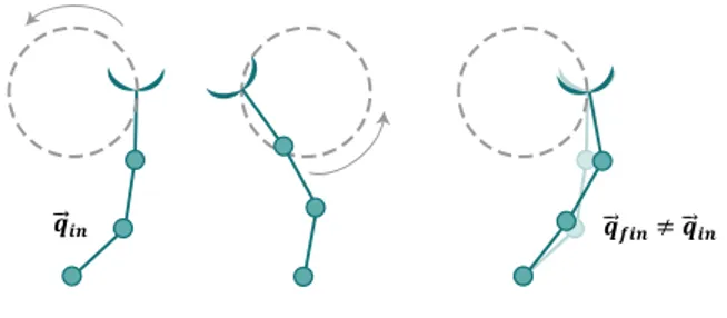
3.1 Jacobian pseudo-inverse method
�𝒒𝒒�⃗𝒇𝒇𝒇𝒇𝒇𝒇≠ �𝒒𝒒�⃗𝒇𝒇𝒇𝒇
�𝒒𝒒�⃗𝒇𝒇𝒇𝒇
Figure 3.1: Example of non-repeatable motion in the joint space
(3.4) as shown bellow:
˙
⃗
q = W−1JAT(JAW JAT)−1⃗x˙d. (3.8)
Pre-multiplying both sides of (3.8) by JA, it is possible to demonstrate that
it satisfies the differential kinematics defined in (2.29). In order to locally minimize the norm of solution, ∥ ˙q∥, it is possible to impose the weighting⃗
matrix W equals to the identity matrix I:
˙
⃗
q = JA†⃗xd˙ (3.9)
As shown in (3.9), the minimum solution is obtained by JA† matrix, which is
defined as the right pseudo-inverse of JA in accordance with Moore-Penrose
properties. It is obtained as follows
JA†= JAT(JAJAT)−1 (3.10)
However the pseudo-inverse of the Jacobian can be computed only when the matrix has full rank, so that, it becomes meaningless when the manipulator is at a singular configuration (the Jacobian matrix contains linearly dependent equations) or also in the neighbourhood of a singularity. Indeed, since it is well known that the computation of the inverse Jacobian matrix requires the determinant matrix value, it becomes a relatively small value in the neighbour-hood of a singular configuration, so that, the joint velocity take high velocity values. In this case, the Singular Value Decomposition (SVD) of JA can be a
valid approach to overcome the problem above described in [55]. An alternative method consists of calculating the Damped Least-Squares (DLS) inverse of the Jacobian matrix JA#, as following defined:
Chapter 3 Redundancy resolution via local optimization
JA#= JAT(JAJAT+ k2I)−1 (3.11)
where k is a damping factor. However, even when the Jacobian has full rank, the (3.10) does not guarantee the repeatability of the end-effector motion. In particular, the example shown in Figure 3.1) demonstrates the loss of motion repeatability (in the joint space) of a planar manipulator, whose final manip-ulator configuration qf in assumed after one tour is different from the initial
manipulator configuration qin. Moreover, it is yet affected by drift error due to
Euler integration (it is directly proportional to simple time value δt). For this reason it is possible to introduce the Jacobian pseudo-inverse JA†(⃗qk) into the
(2.29) in order to obtain the following CLIK expression based on the Jacobian pseudo inverse formulation.
˙
⃗
qk= JA†(⃗qk)( ˙⃗xdk+ K⃗ek) (3.12)
3.2 Jacobian null space method
3.2.1 Jacobian null space projection matrix
The simple CLIK pseudo-inverse in (3.12) does not allow to manage the redun-dant joint motions (motion variables that are not required by the task), which could be used to perform some performance criteria (or secondary tasks), such as: joint limits avoidance, obstacle avoidance and manipulability index opti-mization.
In order to ensure the performance of the primary task, a possible strategy consists in projecting the redundant joints velocity vector requested by the secondary tasks, namely ˙⃗q+k, in the Jacobian null space, N (JA), which is a
subspace of JA having a dimension equals to the degree of redundancy dr, as
defined in (2.7). Since the Jacobian null space is an orthogonal space of the
𝑥𝑥⃗̇𝑑𝑑∈ 𝑅𝑅𝑟𝑟
𝑞𝑞⃗̇ ∈ 𝑅𝑅𝑛𝑛
𝐽𝐽𝐴𝐴
𝑵𝑵( 𝑱𝑱𝑨𝑨 ) 𝑹𝑹(𝐽𝐽𝐴𝐴)
0
Figure 3.2: Relation between joint velocity space and end-effector velocity space
3.2 Jacobian null space method 𝑥𝑥⃗̇ = 𝐽𝐽𝐴𝐴𝑞𝑞⃗̇ 𝐽𝐽𝐴𝐴†𝑥𝑥⃗̇𝑑𝑑 𝑞𝑞⃗̇∗ 𝑞𝑞⃗̇0 𝑃𝑃𝑞𝑞⃗̇0 𝑥𝑥⃗̇ = 𝟎𝟎 𝑞𝑞̇1 𝑞𝑞̇2
Figure 3.3: Geometric view on Jacobian null space
Jacobian image space, namely R(JA), the joint velocities in Jacobian null space
do not produce any velocity on the end-effector. Indeed these joint velocities are linearly mapped by the analytical Jacobian to the end-effector velocity value equals to zero in the Jacobian image space (or Jacobian rank space), as demonstrated in Figure 3.2.
In order to project a secondary task defined by ˙⃗q+k vector into the Jacobian null space of the primary task, it is possible to use the n × n dimensional projector matrix P , such that
JA(⃗qk)Pkq⃗˙
+
k = 0 (3.13)
In particular the P can be obtained at each time instant by:
Pk= I − JA†(⃗qk)JA(⃗qk) (3.14)
where I indicates the identity matrix of suitable dimensions, while the rank of the P matrix is equal to the redundancy degree dr.
The P matrix possesses several properties, as being symmetric (pji = pij),
idempotent (P2= P ) and Hermitian (P−1= P ).
By adding the orthogonal projection of ˙⃗q0in (3.12), it is possible to obtain
the new CLIK expression
˙
⃗
q∗k = JA†(⃗qk)( ˙⃗xdk+ K⃗ek) + Pk⃗q˙0k (3.15)
where the ˙⃗q∗ksolution is different from the one obtained from (3.12), because now it is the minimal norm joints velocity solution that satisfies both the
pri-Chapter 3 Redundancy resolution via local optimization
mary task and the secondary tasks. In particular, a better understanding of (3.12) can be given by the geometric representation in Figure 3.3 (where the
JA†is replaced with J#). In detail, the Figure 3.3 shows a 2-dimensional Joint space, in which the final solution ˙⃗q∗ (red vector) is obtained by the vectorial sum of two vector: the first one is the joint velocity vector with minimum norm (orange vector), while the second one is the orthogonal projection of the secondary task velocity into the Jacobian null space (green vector). Therefore, it is possible to note that the final solution is closest to ˙⃗q0.
3.2.2 Gradient projection method
In the previous section, the ˙⃗q0 vector has been assumed to be arbitrary. A typical choice of ˙q⃗+0
k value is based on the Gradient Projection Method (GPM)
[42]. In detail, this method permits of projecting the gradient of a specific objective function w(⃗qk) (in the joints space), into the Jacobian null space
relative to the primary task. Therefore the ˙⃗q0 results to be equal to:
˙ ⃗ q+0k = ka∇w(⃗qk) = ka ( ∂w(⃗qk) ∂⃗q )T (3.16) where ka is a real scalar value which indicates the gain, and it is a positive
value when w(⃗qk) has to be maximized, otherwise is a negative value if w(⃗qk) has to be minimized [42]. However, the choice of the ka is critical for the
performance of the redundancy resolution. In particular, a small value of the step size may slow down the minimization of the performance criteria w(⃗qk),
while a its large value may even lead to an increase it. An appropriate value of
ka could be chosen by using of in a simplified line search technique as described
in [57].
By replacing the (3.16) in (3.15), the complete GPM expression is obtained:
˙
⃗
q∗k= JA†(⃗qk)( ˙⃗xdk+ K⃗ek) + Pk(ka∇qw(⃗qk)) (3.17)
However the Jacobian pseudo-inverse JA†is yet present in (3.17), hence the
GPM can be computationally intensive, because the SVD has to be generally used. In case the rank of the Jacobian is equal to the task dimension, an alternative method for solving the (3.17) is based on the observation that the redundancy degree is dr. Therefore, the search of the optimum solution ˙⃗q∗k
can be more efficiently performed within a reduced space of the joint variables, which lead to the Reduced Gradient Method RGM ([58]), when rank(JA) =
r. The great advantage of RGM is the use of the simple Jacobian inversion
JA−1that makes it analytically simpler and numerically faster than GPM, but
requires the search for a non-singular minor of the robot Jacobian. 26
![Figure 2.1: Three-link planar arm (revised version of Figure 2.20 from [55])](https://thumb-eu.123doks.com/thumbv2/123dokorg/2969045.27151/28.680.142.512.95.508/figure-three-link-planar-revised-version-figure-from.webp)
![Figure 2.2: Calculation of i − th joint velocity contribution to the end-effector velocity (revised version of Figure 3.2 from [55])](https://thumb-eu.123doks.com/thumbv2/123dokorg/2969045.27151/34.680.142.508.115.331/figure-calculation-velocity-contribution-effector-velocity-revised-version.webp)