3D MHD modeling of twisted coronal loops

2020-07-14T09:01:42Z

Acceptance in OA@INAF

3D MHD modeling of twisted coronal loops

Title

Reale, Fabio; ORLANDO, Salvatore; Guarrasi, M.; Mignone, A.; Peres, Giovanni;

et al.

Authors

10.3847/0004-637X/830/1/21

DOI

http://hdl.handle.net/20.500.12386/26437

Handle

THE ASTROPHYSICAL JOURNAL

Journal

830

3D MHD MODELING OF TWISTED CORONAL LOOPS

F. Reale1,2, S. Orlando2, M. Guarrasi3, A. Mignone4, G. Peres1,2, A. W. Hood5, and E. R. Priest5

1

Dipartimento di Fisica & Chimica, Università di Palermo, Piazza del Parlamento 1, I-90134 Palermo, Italy;fabio.reale@unipa.it 2

INAF-Osservatorio Astronomico di Palermo, Piazza del Parlamento 1, I-90134 Palermo, Italy

3

CINECA—Interuniversity consortium, via Magnanelli 6/3, I-40033, Casalecchio di Reno, Bologna, Italy

4

Dipartimento di Fisica Generale, Università di Torino, via Pietro Giuria 1, I-10125, Torino, Italy

5

School of Mathematics and Statistics, University of St. Andrews, St. Andrews, KY16 9SS, UK Received 2016 April 11; revised 2016 June 27; accepted 2016 July 16; published 2016 October 4

ABSTRACT

We perform MHD modeling of a single bright coronal loop to include the interaction with a non-uniform magnetic field. The field is stressed by random footpoint rotation in the central region and its energy is dissipated into heating by growing currents through anomalous magnetic diffusivity that switches on in the corona above a current density threshold. We model an entire single magnetic flux tube in the solar atmosphere extending from the high-β chromosphere to the low-β corona through the steep transition region. The magnetic field expands from the chromosphere to the corona. The maximum resolution is∼30 km. We obtain an overall evolution typical of loop models and realistic loop emission in the EUV and X-ray bands. The plasma confined in the flux tube is heated to active region temperatures (∼3 MK) after ∼2/3 hr. Upflows from the chromosphere up to ∼100 km s−1fill the core of theflux tube to densities above 109cm−3. More heating is released in the low corona than the high corona and isfinely structured both in space and time.

Key words: Sun: activity– Sun: corona Supporting material: animations

1. INTRODUCTION

Coronal loops are magneticflux tubes where million-degree plasma is confined and are the building blocks of the magnetically closed part of the solar corona. Understanding them means understanding how the corona is structured and powered (see Reale2014, for a review). Each coronal loop is known to evolve fairly independently of nearby ones because the major mass and energy transport processes occur only along the magnetic field lines. This remains true when a coronal loop is modeled as a bundle of thinnerfibrils. Although the fibrils show overall a collective behavior, each of them is thermally isolated from the others. On this basis, coronal loops have been largely investigated as single isolated systems by means of one-dimensional models, where the main role of the magnetic field is to guide the mass and energy transport. This approach has been successful in describing the basic physical processes and many features observed in loops (e.g., Priest 1978; Rosner et al. 1978; Hood & Priest 1979a; Nagai 1980; Doschek et al.1982; Peres et al. 1982; Nagai & Emslie 1984; Fisher et al. 1985; MacNeice 1986; Hans-teen1993; Priest et al.1998; Antiochos et al.1999; Reale et al. 2000b; Bradshaw & Mason2003; Müller et al.2003; Cargill & Klimchuk 2004; Bradshaw & Cargill 2006; Reale & Orlando2008; Guarrasi et al.2010; Reale & Landi2012).

Triggering a loop brightening inside these one-dimensional single-loop models is by an energy input inside a tenuous and cool initial coronal atmosphere. The heating makes the temperature increase rapidly all over the loop because of the efficient thermal conduction, and drives a strong overpressure rapidly down to the dense chromosphere. The chromosphere expands upward andfills the coronal part of the loop with hot denser plasma, so that the loop brightens. The following evolution depends on the duration of the heat release. Continuous heating allows the loop to reach quasi-equilibrium conditions at the highest possible density. With a short heat

pulse the plasma cooling becomes important: after the heating, the temperature decreases rapidly by very efficient conduction, but the density decreases much more slowly, leading to an overdensity over most of the loop’s life. The loops are observed to be bright on timescales longer than the cooling times(e.g., Rosner et al.1978); the question is whether the heat release is really gradual and long lasting, or is instead made of a sequence of short and localized heat pulses distributed in the loop cross-section(Klimchuk2006; Reale2014). In the latter case, the real structure of a loop would be that of a bundle of thinner flux tubes whose thickness is determined by the transverse size of the heat pulse. Evidence for overdensity(e.g., Lenz et al.1999; Winebarger et al.2003), multithermal plasma distribution (e.g., Warren et al. 2011), and some very hot plasma (e.g., Reale et al.2009; Miceli et al.2012; Testa & Reale2012) supports an impulsive heat release, and the question is now turning to how the energy is stored and released, what is the frequency of the pulses, what is the charging mechanism, what is the local conversion mechanism, and whether by the dissipation of waves or by resistive reconnection. Intermittent heating and/or fine structuring is also predicted and discussed by some wave dissipation models, either Alfvén(van Ballegooijen et al.2011; Asgari-Targhi & van Ballegooijen 2012; Asgari-Targhi et al. 2013; van Ballegooijen et al. 2014; Cranmer & Woolsey 2015) or kink modes (Antolin et al. 2014; Magyar & Doorsselaere2016).

A second complementary two-dimensional or three-dimen-sional approach investigates the way the freed magnetic energy powers coronal flux tubes. The stress of a magnetic flux tube has been studied due to twisting (e.g., Rosner et al. 1978; Golub et al.1980; Baty2000; Klimchuk et al.2000; Török & Kliem2003) and braiding of the field lines (López Fuentes & Klimchuk 2010; Bingert & Peter 2011; Wilmot-Smith et al. 2011). Most efforts have been devoted to studying the conditions and effects of the resulting kink instability (Hood

& Priest 1979b; Zaidman & Tajima 1989; Velli et al. 1990; Baty 2000; Gerrard et al. 2001; Török et al. 2004; Bareford et al. 2016), and to the resulting formation of current sheets (Velli et al. 1997; Kliem et al. 2004) and relaxation due to several dissipation mechanisms (Hood et al. 2009; Bareford et al. 2013). MHD simulations have shown the possible importance of local instabilities in the coronal magneticfield to trigger cascades to large-scale energy release (Hood et al.2016).

A third approach is a large-scale one that ranges from the low chromosphere to the corona. It takes the magnetograms and the observations of photospheric granules, and of their dynamics, as boundary conditions to determine the structure and evolution of the upper atmosphere. This approach is able to describe the formation and powering of coronal loops in a qualitative or semi-quantitative way (Gudiksen & Nordlund 2005a; Bingert & Peter 2011), including the emergence of flux tubes by magnetic twisting (Martínez-Sykora et al.2008,2009), so as to reproduce several observed features, such as a constant cross-section (Peter & Bin-gert 2012), and to help interpret and use data analysis tools (Testa et al. 2012). Recent work has supported episodic and structured heating due to the fragmentation of current sheets and/or turbulent cascades (Hansteen et al. 2015; Dahlburg et al.2016).

Evidence for coherent widespread twisting of magneticflux tubes has been found on the solar disk (Wedemeyer-Böhm et al. 2012; De Pontieu et al.2014) and well studied (Levens et al.2015) from optical and UV observations. This represents a natural stressing mechanism of the magnetic field that eventually leads to a relaxation and a release of magnetic energy (e.g., Rosner et al.1978; Golub et al.1980; Klimchuk et al.2000; López Fuentes et al.2003).

Here we set up a numerical experiment for a coronal magnetic flux tube that is anchored in the chromosphere and progressively twisted by the rotation of the plasma at the footpoints. Our approach is a step forward from one-dimensional loop modeling to allow an active role for the magneticfield, including the expansion of the field lines in the transition region and the energy production from field dissipation. Our choice has been to assume a relatively simple setup but still including many ingredients of a loop heated by magnetic dissipation. A coherent rotation of the footpoints with some moderate perturbation allows us to have some control on the effects in such a complex MHD system. As new achievements with respect to other previous MHD modeling of twisted loops, our modeling includes a highly non-uniform solar atmosphere and magnetic field with the boundary in the chromosphere. A fundamental target of our work is to reproduce the full typical evolution of a coronal loop, including the chromospheric evaporation driven by magnetic heating excess. This is not an easy task because it requires high spatial resolution (Bradshaw & Cargill 2013) in a three-dimensional (3D) MHD framework. Our model also aims at accurately describing the temperature stratification and evolution to synthesize observables for diagnostics and direct comparison with observations.

We consider a complete loop atmosphere with a corona connected to two thick chromospheric layers by thin transition regions, immersed in a magnetic field. The magnetic field is arranged to be mostly uniform in the corona and strongly tapering in the chromosphere, where the ratio of thermal to

magnetic pressure switches from low to high values (β > 1). Therefore, our model accounts for the interaction with the magnetic field including the critical region where β changes regime. The model also includes heating mechanisms that derive from the dissipation of the magneticfield. The heating is basically determined by the anomalous diffusivity that reconnects the magneticfield above a current density threshold. The currents grow because of the progressive twisting of the magneticfield. The field is twisted by random rotational plasma motions at the loop footpoints, which drag thefield. We show that this magnetic stress and dissipation drives a typical coronal loop ignition, structuring, and evolution.

2. THE MODEL

We consider a box containing a single coronal loop. For simplicity of modeling, the loop is then straightened into a magnetic flux tube rooted in the photosphere through two chromospheric layers at opposite sides of the box(top and bottom boundaries; Guarrasi et al.2014). These two layers can be treated independently since the loop footpoints are far from each other and therefore located in independent regions of the chromosphere and photosphere. We consider only the gravity component along theflux tube and, in particular, that of a curved (semicircular) flux tube, i.e., it decreases to zero at the midpoint. This assumption holds as long as the twisted region has a small cross-section with respect to the tube length, as it is in this case.

Our domain is a 3D cylindrical box (r, f, z). The box is much broader than the cross-section of the loop. The evolution of the plasma and magnetic field in the box is described by solving the full time-dependent MHD equations including gravity(for a curved loop), thermal conduction (including the effects of heatflux saturation), radiative losses from optically thin plasma, and an anomalous magnetic diffusivity.

The MHD equations are solved in the non-dimensional conservative form: · ( ) ( )  r r ¶ ¶t + u =0 1 · ( ) ( )  r _{r r} ¶ ¶ + - + = u uu BB I g t Pt 2 · [ ( ) ( · )] · [( · ) ] · · ( ) ( )    r _r h r ¶ ¶ + + -= - ´ + - - L + u B v B J B u g F E t E P n n T Q 3 t c e H · ( ) ( · ) ( )   h ¶ ¶ + - = - ´ B uB Bu J t 4 · ( )  B=0 5 where · ( ) = + B B P p 2 6 t ( )  p = ´ J c B 4 7 · · ( )  r = + u u + B B E 2 2 8 ∣ ∣ ( ) = + F F F F F 9 c sat sat class class ˆ ( ˆ · ) [ ˆ ( ˆ · )] ( ) ∣∣    = + ^ -Fclass k b b T k T b b T 10

∣Fclass∣= ( ˆ ·b T) (2 k_∣∣2-k_^2)+k_^2T2 (11) ( ) fr = Fsat 5 ciso 12 3

are the total pressure(Pt), induced current density (J), and total energy density E (internal energy ò, kinetic energy, and magnetic energy), respectively, p is the thermal pressure, t is the time, nH and ne are the hydrogen and electron number density, respectively, ρ=μmHnH is the mass density, μ=1.265 is the mean atomic mass (assuming metal abundance of solar values, Anders & Grevesse 1989), mH is the mass of hydrogen atom, u is the plasma velocity, B is the magneticfield, ˆb is the unit vector along the magnetic field, g is the gravity acceleration vector for a curved loop, I is the identity tensor, T is the temperature, η is the magnetic diffusivity, Fcis the thermal conductiveflux (see Equations (9)–

(12)), the subscripts ∣∣ and ^ denote, respectively, the parallel and normal components to the magneticfield,k =K T5 2_and

( )

r =

^ ^

k K 2 B T2 1 2 _{are the thermal conduction coefficients} along and across the field, K =9.2´10-7 _and

= ´

^

-K 5.4 10 16 _{(cgs units), ciso is the isothermal sound} speed,f=1 is a free parameter, and Fsatis the maximumflux magnitude in the direction of Fc.L T represents the optically( )

thin radiative losses per unit emission measure derived from the CHIANTI v.7.0 database (e.g., Dere et al. 1997; Reale et al. 2012; Landi et al. 2013) assuming coronal element abundances (Feldman1992). Q=4.2×10−5erg cm−3s−1is a volumetric heating rate sufficient to sustain a static corona with an apex temperature of about 8×105 K, namely a background atmosphere adopted as initial conditions, accord-ing to the hydrostatic loop model by Serio et al.(1981; see also Guarrasi et al. 2014). An estimate of this heating rate can be derived from loop scaling laws(Rosner et al.1978; Reale2014) that can be rearranged intoQ~10-3T L

-6 3.5

9 2

, where T6and L9 are the temperature and the loop half-length in units of 106K and 109cm, respectively.

This heating rate is much lower than the one produced by coronal twisting. We use the ideal gas law, p=(γ − 1) ρò. We assume negligible viscosity, except for that intrinsic in the numerical scheme.

The calculations are performed using the PLUTO code (Mignone et al. 2007,2012), a modular, Godunov-type code for astrophysical plasmas. The code provides a multiphysics, algorithmic modular environment particularly oriented toward the treatment of astrophysical flows in the presence of discontinuities of the kind present in the case treated here. The code is designed to make efficient use of massive parallel computers using the message-passing interface library for interprocessor communications. The MHD equations are solved using the MHD module available in PLUTO, configured to compute intercell fluxes with the Harten–Lax–Van Leer approximate Riemann solver, while second order in time is achieved using a Runge–Kutta scheme. A Van Leer limiter for the primitive variables is used. The evolution of the magnetic field is carried out adopting the eight wave formulation introduced by Powell et al. (1999), which maintains the solenoidal condition ( ·B=0 at the truncation level.)

PLUTO includes optically thin radiative losses in a fractional step formalism (Mignone et al. 2007), which preserves the second-order time accuracy, since the advection and source

steps are at least second-order accurate; the radiative loss Λ values are computed at the temperature of interest using a table lookup/interpolation method. The thermal conduction is treated separately from advection terms through operator splitting. In particular, we adopted the super-time-stepping technique(Alexiades et al.1996), which has been proved to be very effective to speed up explicit time-stepping schemes for parabolic problems. This approach is crucial when high values of plasma temperature are reached (as during flares), the explicit scheme being subject to a rather restrictive stability condition (i.e., Dt(Dx)2 2h _{where η is the maximum} diffusion coefficient), since the thermal conduction timescale τcond is typically shorter than the dynamical one τdyn (e.g., Orlando et al.2005,2008).

Our main simulations required about 30 million hours on 32000 cores of the CINECA/FERMI Blue-Gene high-performance computing system.

2.1. The Loop Setup

We describe a box that contains a typical active region loop, with total length of the coronal section 2L=5×109cm, which is driven to a temperature T∼3×106K. The loop atmosphere includes a coronal part that is connected to the chromosphere through a steep transition region. In our configuration the corona is between two independent chromo-spheric layers, at opposite sides of the geometric domain. Initially, the loop is relatively tenuous and cool: its atmosphere is plane-parallel and hydrostatic (Serio et al. 1981) with an apex temperature about 8×105K. In the transition region the temperature drops to 104 K in less than 108 cm. The temperature is uniform at 104 K in the chromosphere. The density correspondingly increases from ∼108cm−3 in the corona to ∼1011cm−3 in the upper chromosphere and ∼1014_cm−3_{in the lower chromosphere.}

We consider a magneticfield that expands upward along the loop because of the change ofβ regime from the chromosphere to the corona. To obtain this as initial condition for our modeling, we follow the same procedure as in Guarrasi et al. (2014), i.e., we carry out a preliminary 2.5D simulation in cylindrical geometry that starts from a magneticfield with field lines running parallel along the loop. This initial magneticfield links the two chromospheres, but its intensity and the background pressure are more intense in the central part of the loop(around the symmetry axis) than in the surroundings. In this simulation, we let this system evolve, and it relaxes to a new equilibrium: the magnetic field expands considerably in the corona, because the internal total pressure is higher than outside, until the system is again in equilibrium, i.e., the maximum plasma velocities are not larger than a few km s−1 everywhere in the domain. Finally, we map the 2.5D simulation output into the 3D domain.

At the end of this preliminary step, the loop is in a new equilibrium: the plasma stratification is very similar to the previous hydrostatic one, but now the magnetic field lines expand from chromosphere to the corona around the loop central axis. The magneticfield intensity decreases from ∼300 G at the bottom of the chromosphere to∼60 G in the transition region and to∼12 G (still sufficient to confine the loop plasma) at the top of loop, i.e., in the middle of the domain. The area expands by a factor of six from the bottom of the chromosphere to the top of the transition region, another factor of two in the first 3000 km above the transition region, and a further factor of

two to the top of the loop (middle of the domain). Figure 1 shows the equilibrium conditions from which we start the loop twisting. In this and the followingfigures the loop is presented as “straightened” with the two footpoints and chromospheric layers at the top and bottom of thefigure, and the coronal loop between. The magneticfield is more intense around the central axis and the atmosphere readjusts there to a slightly higher coronal temperature and lower density than those reported at the beginning of this section(the initial atmosphere around the central axis is shown as black lines in Figure9). The field lines clearly show the tapering from the corona to the chromosphere. The computational domain is 3D cylindrical (r, f, z, Figure 1). In order to obtain a good compromise between adequate resolution and reasonable coverage of the azimuthal (f) domain we model only one quadrant with periodic boundary conditions. We also skip the singular central axis, and consider an inner boundary radius r0>0. In the end, the domain range is -zM< <z zM along the loop axis where

zM=3.1×109cm,r0=7 ´107 r rM=3.5´109 cm across the loop, and0f90 in the azimuthal direction.

To describe the transition region at sufficiently high resolution (Bradshaw & Cargill 2013), the cell size there (∣ ∣ »z 2.4´109 _{cm) decreases to dr~dz~3´10}6 _cm. The resolution is uniform in the angle f, i.e., f » d 0 . 35.

We adopt reflective boundary conditions at r=r0, i.e., close to the symmetry axis; reflective boundary conditions at r=rM; periodic boundary conditions at f= 0 and f =90 ; and reflective boundary conditions but with reverse sign for the tangential component of the magneticfield at z=±zM.

2.2. Loop Twisting

The aim of this work is to trigger heating and brightening of a coronal loop through progressive stressing of the magnetic field twisted at the footpoints. The dissipation is due to anomalous magnetic diffusivity, and grows because the twisting amplifies induced electric currents. The twisting is driven by a rotational plasma motion at both footpoints. The

driver is photospheric and the rotational motion is set at the lower and upper boundaries of the domain, which can be considered as the boundaries between the photosphere and the chromosphere.

The basic rotation profile is that of a rigid body around the central axis, i.e., the angular speed is constant in an inner circle and then decreases linearly in an outer annulus. More specifically, at the lower and upper boundaries, the velocity component alongf is defined as

( ) ( )

å

where the sign is positive (negative) at the lower (upper) boundary, ( ) w = ´ < - < < > ⎧ ⎨ ⎪ ⎩⎪ v R r R R r R R r R r R 1 2 2 0 2 . max max max

max max max max

max

The parametersαiare random numbers between 0 and 30:

[ ]

a = 23, 9, 0.6, 15, 19, 13 and vmax=5 km s−1 _{and Rmax=3000 km.}

The angular speed ω was chosen so that the maximum tangential speed is v(0, Rrot, t)=5 km s−1, in agreement with typical photospheric granule speeds(Muller et al.1994; Berger & Title 1996). The rotation period of each footpoint is Trot≈1 hr. The rotational motion is the same but in the opposite direction at the other boundary, i.e.,

( )= - ( )

v Zmax, ,r t v 0, ,r t . Since we have equal but opposite motions at the two footpoints, the relative rotation speed of one footpoint with respect to the other is twice, i.e., 10 km s−1, and the rotation period is half, i.e., ∼1/2 hr. The input Poynting flux through each rotating footpoint grows linearly to Fx∼3.1×107 erg cm−2s−1 at the final time t∼2500 s. Thefinal total rotation angle is ≈2.7π.

For a more realistic speed pattern, we perturb the velocity through a combination of random sinusoidal functions that depend on f and r. The amplitude of these perturbations is 20%. The rotation velocityfield is shown in Figure2.

2.3. The Plasma Resistivity

For our reference simulation of this work we consider an anomalous plasma resistivity that is only switched on when the magnitude of the current exceeds a critical value as in the following(Hood et al.2009):

∣ ∣ ∣ ∣ ( )  h= h < ⎧ ⎨ ⎩ ⎫ ⎬ ⎭ J J J J 0 14 0 cr cr

where we assumeη0=1014cm2s−1 and Jcr=75 A cm−2. With this assumption the minimum heating rate above switch-on is H=h₀(4p∣ ∣Jcr c)2 »0.1erg cm−3 s−1, corresp-onding to a maximum temperature of ∼6 MK for an equilibrium loop with half-length 2.5×109cm, according to the loop scaling laws (Rosner et al.1978). Below the critical current, a minimum numerical resistivity is anyway present, but it does not produce perceptible heating during the simulation. For comparison, we made a simulation also with a constant and uniform resistivity in the corona(Bingert & Peter2011); we set η=1013

cm2s−1, which corresponds to a magnetic Reynolds number RM∼1 for typical speeds of ∼10 km s−1 and scale Figure 1. Temperature (left, [MK], linear scale) and density (right, [109_cm−3_],

logarithmic scale) color map in a transverse plane across the loop axis, before the footpoints begin to rotate and twist the magneticfield. The chromosphere is red in the density map and blue in the temperature map. The magneticfield lines are marked(green lines).

lengths of ∼100 km. In the chromosphere we assume a perpetual perfect equilibrium of energy losses and gains, and therefore we assume a resistivity η=0 there. Although the currents are larger in the chromosphere, their dissipation would not increase the chromospheric temperature significantly because of the very high heat capacity of the dense chromo-spheric plasma. On the other hand, the current dissipation

would weaken considerably the magneticfield, and we have no way to replenish it from below as in the real Sun. Our choice allows us to maintain a sufficiently strong magnetic field throughout the simulation and thus to sustain the coronal heating for a sufficiently long time to reach high temperatures.

3. THE RESULTS

We model the 3D MHDflux tube (loop) evolution until the loop plasma reaches a maximum temperature T∼4 MK, i.e., in the time range 0<t<2500 s.

The footpoint rotation starts at time t=0. The rotation drags the magneticfield anchored at the footpoint and the field lines begin to twist since β∼100 there (Figure 3). The twisting propagates upward at the Alfvén speed, whose profile along the flux tube is shown in Figure3. Below the corona, the Alfvén speed varies steeply from ∼2 to ∼2000 km s−1. The perturbation takes about 200 s to propagate along a vertical distance of∼7000 km to above the transition region, i.e., with an average speed of∼35 km s−1.

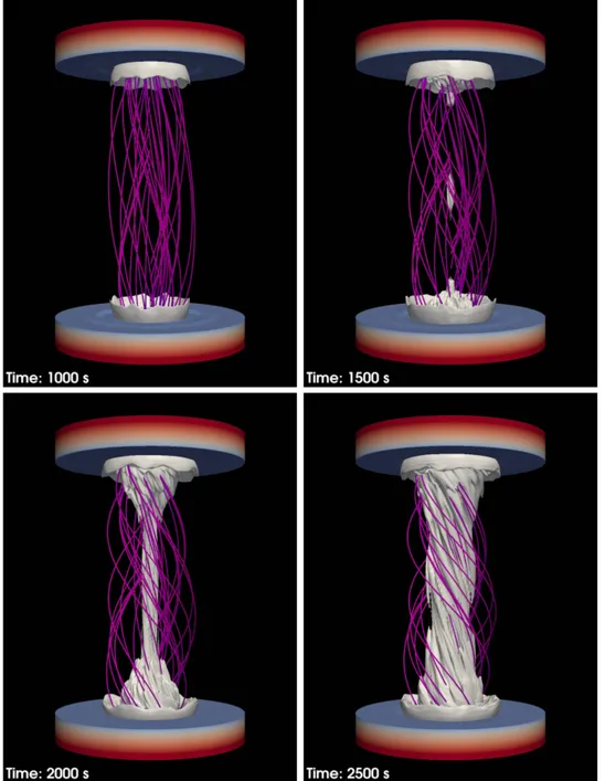
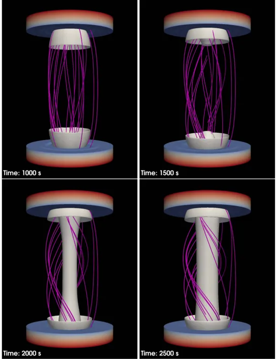
The progressive twisting of the magnetic field makes the current density gradually increase as well, according to Equation(7). It takes several minutes for the current to grow above the critical value in the corona, which triggers the dissipation into heating. Figure 4 shows snapshots of current surfaces at four progressive times during the evolution. The figure shows the current surfaces at the critical value for dissipation. Although the computational domain extends over an angle of 90°, for the sake of clarity we replicate the image to cover all 360°. The currents are more intense in the low part of theflux tube, where the magnetic field expands and the twisting is driven. The current density first increases in the shell boundary layer of the twisted region (i.e., at r ∼ 6000 km), where there is a shear between twisted and untwisted region (t = 1000 s). Later, the current intensity increases more significantly in the core of the flux tube, as the twisting becomes more and more effective(t = 1500, 2000 s). Current intensification propagates from the footpoints upward all along theflux tube.

As a consequence of the random twisting, the current does not grow uniformly, but it develops into long irregular structures along the field lines, best visible at the final time (t = 2500 s). As soon as the current threshold for dissipation is exceeded, the magnetic field lines progressively reconnect in the corona, where the heating is released. According to Figure 2. Rotation velocity field. Top: color map of vf; middle: velocity profile

along r forf=45° (along the dashed line in the top panel) with (dashed line) and without(solid line) random perturbations; bottom: velocity profile along f for r=3×108_{cm(along the dotted line in the top panel) with (dotted line)} and without(solid line) random perturbations.

Figure 3. Profile of plasma β (solid) and Alfvén speed (dashed) along the central axis of the domain.

Schindler et al. (1988), a signature of the reconnection is the integral of the parallel component of the electric field along the magneticfield lines (

ò

of light. Typical values of the electric field can be estimated from the Ohm’s law and using the critical current ∣ ∣E =4ph_{0 cr}∣ ∣J c2 ~p105 _{statV/cm. We find that the integral} progressively rises with time from∼1013to∼1015statV, where the heating is on (and zero elsewhere), confirming substantial reconnection.

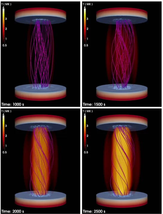
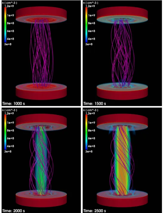
Figures 5 and 6 show snapshots of the plasma temperature and density at the same times as Figure 4. The temperature

begins to increase significantly at t∼1500 s and, first, in a shell at the boundary of the twisted region, because of the shear between twisted and untwisted layers. The heating of this outer shell remains quite low throughout the subsequent evolution and the shell is not significantly activated. With some delay, the inner part of the twisted magnetic cylinder is heated and the heating there is more efficient. The inner twisted region becomes hotter quite uniformly all along the flux tube axis because of the efficient thermal conduction along the field lines in the corona. The evolution of the density is more gradual, i.e., it increases significantly at later times. The density increases because the heating produces an overpressure inside the twisted Figure 4. Current density surfaces (white) at the critical value for dissipation (∣ ∣ =Jcr 75A cm−2) at four different times during the twisting of the coronal loop. The images result from the replication of the original 90°domain. Only the region around the central axis is shown. The twisting is around the central vertical axis and the chromosphere appears as two thick solid(colored) disks at the top and bottom of the domain. Magnetic field lines are also shown (pink lines, see Animation 1 in the online journal).

region, and therefore an expansion of the dense lower layers upward to the tenuous corona, the so-called chromospheric evaporation.

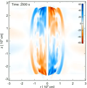
The plasma moves along the magnetic field lines and the twisting of thefield makes the motion a spiraling one, adding a significant component along f. Figure 7 clearly shows this spiraling component of the upflows from the chromosphere, which would produce blue- and redshifts if the loop is viewed from the side, as found in recent observations of twisting motions(De Pontieu et al.2014).

The density never grows much above∼3× 108cm−3in the outer shell of the twisted tube. In the core, instead, the coronal density gradually increases to higher values(∼109cm−3), filling the space between the chromospheres. In the end, a proper

coronal loop forms, with a dense and hot inner cylindrical region and a thin and more tenuous shell. Looking carefully, especially at the footpoints, at time t=2500 s, it is possible to distinguish some fine structuring, due to the jagged current dissipation (Figure4). The fine structure is less remarkable up in the corona both because of the efficient thermal conduction along the field lines and because of the cross-field dispersal driven by the reconnection(Schrijver2007).

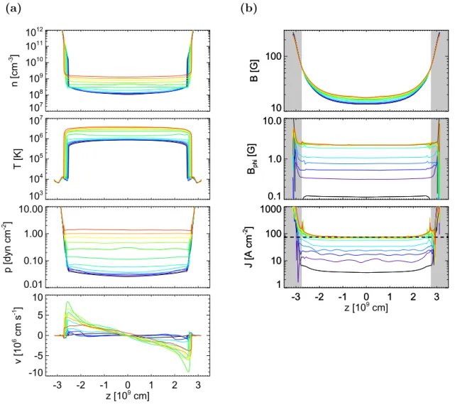
Figure 8 shows radial profiles of the density, temperature, pressure, magneticfield intensity, azimuthal component of the magneticfield, and current density at the top of the loop and at the end of our simulation. The inner region is the one with the highest values of most quantities, as expected. The first four profiles show a decay from the central axis, to reach a value Figure 5. Temperature rendering at the same times and in the same domain as in Figure4. The units are[106K]. Magnetic field lines are also shown (pink lines, see Animation 2 in the online journal).

close to the ambient one at r>109cm. The density decreases more rapidly, because the heating is more effective close to the central axis. The temperature decreases instead more smoothly, as is also perceptible in Figure5. The azimuthal component of the magnetic field provides information about the twisting along the loop. The profile at the loop apex is very similar to the unperturbed rotation profile shown in Figure 2 (middle panel), but widens to a larger radius because of the expansion of the magneticfield. The current density profile is flat around the critical value for dissipation, Jcr, to r∼3×108cm, which is also where the density is the highest. A secondary peak of T, p, n, and J is found at r∼1.2×109cm, and drops at the boundary between the twisted and untwisted region. The pressure halves at r∼4–5×108cm, which may be taken as

an effective loop width. The magneticfield is amplified by a factor of 1.5 around the central axis.

Figure 9 shows profiles of plasma density, temperature, pressure, and vertical velocity, and of the total magneticfield intensity, the azimuthal component of the magneticfield, and the current density near the central vertical axis of the magnetic flux tube at equi-spaced times. The central axis is a very good approximation of afield line at any time, so we are also looking at the evolution along a field line. From Figure9(a) the loop plasma remains quite steady for a relatively long time at the beginning of the simulation, when the twisting is still unable to provide current dissipation. After several hundreds of seconds (pale blue, green lines), the current density increases above the threshold for dissipation in the low corona (i.e., for Figure 6. Density rendering at the same times and in the same domain as in Figure4. The units are[109cm−3]. Magnetic field lines are also shown (pink lines, see Animation 3 in the online journal).

∣ ∣ »z 2.6´109_{cm), as shown in Figure9(b), while this occurs} earlier at larger radial distances from the central axis. Above this threshold, the heating turns on impulsively, and the density, temperature, and pressure all begin to increase rapidly.

The profiles are typical of the evolution from standard loop models(e.g., Reale et al.2000a; Warren et al. 2002; Spadaro et al.2003; Guarrasi et al.2014). The temperature and density appear to increase almost simultaneously because the evapora-tion of chromospheric plasma occurs in times smaller than the time spacing of thefigure (e.g., Reale2014). The evaporation speeds are higher close to the footpoints. They increase initially up to almost 100 km s−1and then begin to settle down to more moderate values below 50 km s−1.

Once the heat release has started, the thermal pressure increases regularly and eventually grows above 1 dyne cm−2in the corona. Figure 9(b) shows that the magnetic field is progressively twisted, i.e., B_f increases, uniformly in the corona. It also shows that the total coronal magnetic field increases as well by about 50%, while it does not at the footpoints. The twisting of the magneticfield leads to a boost of the current density in the corona, which is the origin of the heating.

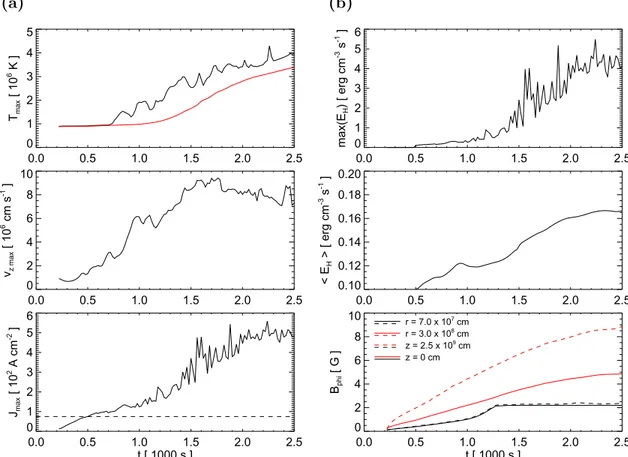
Figure 10(a) shows the evolution of the maximum loop temperature, maximum vertical speed and maximum current density in the region where the dissipation is allowed, i.e., above the transition region. The maximum current density has an increasing trend until t∼2000 s, although with strong fluctuations at late times. Then it seems to become steady. The threshold for dissipation is reached at t=th≈500 s and at the end of the simulation the maximum value is above 500 A cm−2. Figure9(b) shows that these high values are localized in the low corona.

The maximum temperature is initially steady at∼1 MK and it begins to increase with an irregular trend at time t≈700 s, taking about t∼1000 s to settle around the maximum of ∼4 Figure 7. Color map of the velocity component [km s−1_{] along f in a}

transverse plane across the loop axis(see Figure1) at time t=2500 s (blue is

outward from thefigure, red is inward).

Figure 8. Radial profiles of (a) density, temperature, and thermal pressure, and (b) magnetic field intensity, azimuthal component of the magnetic field, and modulus of the current density, at the top of the loop(z = 0), for f=45°, and at time t=2500 s. The current threshold for dissipation is marked (dashed line).

MK, a hot active region loop. In spite of the slight delay, the overall temperature trend resembles quite closely the one of the maximum current. The top panel of Figure10(a) shows also the average temperature at the loop apex, which gives an idea of the average conditions of the loop. This temperature begins to rise for t>1000 s and reaches a value above 3 MK at the end time, typical of active region loops. From Figure10(a) we see that the maximum temperature does not rise as long as the resistivity is off. Therefore, the effect of the enhanced magnetic tension due to the twisting is low, at least in the corona.

The maximum vertical speed provides information about the strength of the evaporation. It begins to increase readily at t≈thand takes about 1000 s to settle to∼80–100 km s−1, with a slightly decreasing trend for t>1500 s. These relatively high values of speed are typical of impulsive evaporation, driven by a continuous sequence of heat pulses (e.g., Patsourakos & Klimchuk 2006).

Figure 10(b) shows the evolution of the maximum heating rate and of the heating rate averaged only over the heated cells, i.e., with EH> 0 and r<109cm. The evolution of the maximum heating rate resembles closely that of the maximum

current density(Figure10(a)), with spikes reaching very high values(∼5 erg cm−3 s−1). Each spike represents an impulsive energy release. The duration of each pulse is less than a minute, and these are the high-energy tails of a distribution that provides the average heating rate produced by the twisting and shown in the bottom panel of Figure10(b). This average rate increases by about 60% throughout the simulation. In the last panel, Figure 10(b) shows the evolution of the azimuthal component of the magneticfield Bf, i.e., of the twisting, at two different heights along the loop (apex and just above the transition region) and at two different radial distances from the central loop axis(close to the axis and 3000 km apart). At first B_finvariably increases at all position, more rapidly far from the axis because the rotation is faster there. At time t∼1300 s it saturates close to the loop axis, because of the dissipation. Farther from the axis the curves saturate much later, close to the end of the simulation. There, B_fgrows less at the apex than at the bottom, because of the field expansion, i.e., the field is weaker at the top than below. Close to the axis, instead, the expansion is small and the field component grows more uniformly.

Figure 9. Evolution of (a) the plasma density, temperature, thermal pressure, and vertical velocity, and (b) of the total magnetic field intensity, the azimuthal component of the magneticfield, and the current density, close to the central vertical axis of the twisted flux tube. The profiles are spaced by 200 s and the color coding marks the time progression, from black(t = 0) to red (t = 2500 s). Positive velocity is to the right, i.e., upward from the left footpoint. The critical current density and the region where the resistivity is zero are marked(horizontal dashed line and gray strips, respectively).

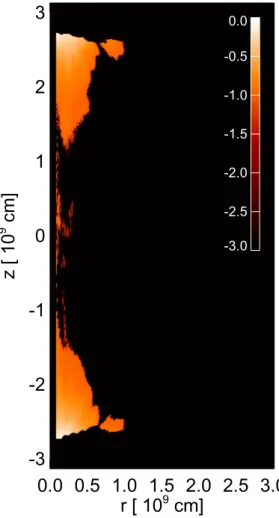
Figure 11 shows information about the distribution of the heating release at thefinal time, which can be compared to the current distributions shown in Figures 4 and 9. The figure shows the cross-section of the heating distribution across the central axis in the r−z plane. The heating is clearly broader and more intense near the loop footpoints, and some minor quantity is released along the central axis. Some heating is also released for r>5×108cm, only close to the footpoints. Figure12shows the temperature and density and the emission predicted from a slice across the loop central axis in two EUV (SDO/AIA 171 Å and 335 Å) channels and in one X-ray (Hinode/XRT Ti_poly) channel. In the 171 Å channel, sensitive to plasma at∼1 MK, the loop is practically invisible. We only see a faint halo in the outer shell and bright layers at the footpoints. This is expected because the loop plasma is mostly at temperatures around 2–3 MK, and therefore only the thin transition region emits in this channel. The 335Å channel is more sensitive to plasma hotter than 2 MK and the loop is fully visible and bright in this channel. For the same reason it is analogously bright in the X-ray band: here only the central region is bright because this channel is more sensitive to higher temperature plasma. The emission predicted in these two channels is fairly uniform in the body of the loop, and the loop appears as monolithic. Some inhomogeneity and tapering is present close to the footpoints.

3.1. Comparison with Constant Resistivity and Uniform Rotation

To understand the role of the selected heated mechanism, we have compared the reference simulation above with another identical one(hereafter CRS) except for two issues: (a) the resistivity is constant and always on in the corona (see Section 2.3), with no current threshold, and a value η=1013_cm2_s−1_{, i.e., 10 times lower than the switch-on} value(Section 2.3); (b) the velocity field at the footpoints is not random, i.e., there is a uniform rotation motion. This choice implies a radial symmetry around the central vertical axis, and we actually obtain a radially symmetric evolution. According to this simulation, theflux tube is gradually heated to coronal temperature and filled with plasma from the chromosphere. All this evolution occurs more gradually and uniformly than in the reference simulation. Figure 13 shows that the current density grows from the loop footpoints upward and eventually it is uniformly high all along the loop axis. Thefine structure that we see in Figure4is purely due to the perturbations of the rotation motion at the footpoints, which are not present in the simulation of Figure13. Figure14 shows other interesting features from the comparison with the reference case (Figure 10). The temperature regime is analogous, so the comparison is sound, but the reference case shows higher peaks, above 4 MK. The reference Figure 10. Evolution of (a) the maximum temperature, vertical velocity, and coronal maximum current density in the simulated box, and (b) of the maximum heating rate per unit volume(top), the averaged heating over cells with EH> 0 and r<109cm(middle, black solid lines), and of the azimuthal component of the magnetic field Bf, forf=45°, at the two labeled heights z along the loop, i.e., apex (solid) and just above the transition region (dashed) and at the two labeled radial distances r from the central axis, i.e., close to the axis(black) and 3000 km far away (red). In panel (a) the average temperature at the loop apex (red line) and current threshold for dissipation(horizontal dashed line) are also shown.

simulation also yields much higher evaporation speeds and currents(more than twice as high on average). This difference is due to the presence of the threshold for current dissipation,

which lets the magneticfield be stressed more and energy be released more impulsively.

4. DISCUSSION AND CONCLUSIONS

This work describes a possible scenario of a coronal loop heated by magnetic field stressing. This is an evolution from the standard one-dimensional single- or multi-strand loop modeling(see Section1) and a step forward in self-consistent MHD loop modeling. Single-loop models describe the hydrodynamics of a coronal atmosphere linked to the chromo-sphere through a steep transition region confined in a curved flux tube. The curvature appears only in the formulation of the gravity. The plasma moves and transports energy only along the tube, under the effect of a prescribed heating function. Here we maintain the same plasma atmosphere but we immerse it in an ambient “cylindrical” magnetic field, which expands from the chromosphere up into the corona, as in Guarrasi et al. (2014). We no longer consider a prescribed heating function, but the heating is a consequence of stressing the magneticfield. This provides a self-consistent conversion of magnetic energy into heat. Our choice has been to start from simple, but realistic, assumptions on magnetic stressing and energy conversion: the magneticfield is stressed through the twisting driven by rotational footpoint motion in layers where plasma β?1; twisting is believed to be quite usual in the solar atmosphere (Wedemeyer-Böhm et al. 2012; De Pontieu et al. 2014). The rotation motion is perturbed as expected in the solar surface, and this is fundamental to break the symmetries and let currents fragment into sheets (Nickeler et al.2013; Rappazzo et al.2013). The sheets are progressively intensified by the twisting and this occurs more at the loop footpoints where the magnetic field is tapered, crossing the transition region to the chromosphere. In this scenario we have hypothesized a switch-on dissipation mechanism. Heating from a very high anomalous resistivity is released as soon as the current density grows above a given threshold (Hood et al. 2009), which we set to 2.25×1011 esu s−1cm−2, to mimic possible turbulent cascades or MHD avalanche Figure 11. Cross-section in the r–z plane across the loop central axis of the

volumetric heating rate, EH, at t=2500 s (log scale).

Figure 12. From left to right: cross-sections of the temperature and density, and of the synthetic emission (log scale), in the SDO/AIA 171 Å and 335 Å channels and in the Hinode/XRT Ti_poly filter band, at t=2500 s. The emission units are DN cm−1s−1pix−1.

(Rappazzo & Parker 2013; Hood et al. 2016). Since here we address mostly the coronal evolution, the heating is assumed (in common with some previous simulations) to be active in the corona only, just because otherwise the magnetic field in the chromosphere is rapidly dissipated and we have found no way to refurbish it.

Our single-loop study supports other findings from MHD modeling of solar atmosphere boxes (e.g., Hansteen et al.2015), and provides fine details. We start from a tenuous and cool atmosphere. Where the current grows above the threshold in the corona, the plasma begins to heat above 1 MK. The heating is more steady and efficient around the loop central axis, where the temperature rises above 3 MK on average in about half an hour. At the same time, the increasing pressure gradients determine the expansion of the chromospheric layers and the tube fills with denser plasma. The density gradually

rises above 109cm−3. This evaporation is in agreement with standard single-loop models. From comparison with an equivalent simulation with ever-present anomalous resistivity, we have ascertained that the presence of the switch-on heating that leads to a factor-of-two larger evaporation speeds, even in the late steady state. This is therefore a major difference between a gradual and an impulsive heating mechanism. Another important difference is the presence of overheated plasma. At variance from the gradual-heating simulation, the switch-on heating produces some amount of plasma signi fi-cantly hotter than the average, as expected from impulsive heating(Klimchuk2006) and recently detected in bright active regions(e.g., Reale et al.2009,2011; Miceli et al.2012; Testa & Reale2012).

The heating is more intense where the magneticfield is more intense, i.e., close to the footpoints, where it expands more. Figure 13. Current density for the simulation with constant coronal resistivity and unpertubed footpoint rotation to be compared with Figure4.

This is in agreement with other MHD modeling of the solar atmosphere (Gudiksen & Nordlund 2005a,2005b; Bingert & Peter 2011, 2013). The heating is more intense around the central axis where the footpoint rotates and the twisting of the magnetic field is effective. The energy release determines a progressive dissipation of the magneticfield, through the local reconnection of sheared field lines. With our choice of magnetic diffusivity, this dissipation drives the plasma to density and temperature typical of active regions already at moderate twisting angles, far from the conditions to trigger kink instabilities (Hood & Priest1979b,1981; Einaudi & van Hoven1983; Velli et al.1990; Török & Kliem2003).

The kink instability has been suggested as a trigger mechanism for the rapid heating of coronal loops. Hood et al.(2009) have shown that its nonlinear development creates current sheets, and triggers magnetic reconnection. Once reconnection starts, the current sheets fragment, resulting in the dissipation of magnetic energy across the loop cross-section, as it relaxes toward its lowest energy state. Starting from a temperature of only 104K, their results show that plasma heating up to 107K and above is possible. Botha et al. (2011) included thermal conduction so that lower temperatures were obtained.

In addition to previous twisting models, our description includes the chromosphere and the transition region at reasonable resolution. Another important ingredient is the expansion of the magneticfield from the chromosphere to the corona(Rosner et al.1978), which, together with the change of

β regime in the chromosphere, stresses the importance of the nonlinear interaction of the plasma and the magneticfield. Our model is also able to describe a significant mass transfer from the chromosphere to the corona, an essential feature for comparison with the observed loops brightness. The plasma produces realistic emission in X-ray and EUV bands. Its evaporation and the twisting drive significant spiraling motions as recently extensively observed(De Pontieu et al.2014).

Our choice here is to produce loop heating with a relatively ordered magnetic stressing, i.e., the progressive random twisting due to footpoint rotation. So we are not describing an entirely chaotic magnetic stress, determined by random photospheric motions that lead to magnetic braiding (López Fuentes & Klimchuk 2010; Bingert & Peter 2011; Wilmot-Smith et al. 2011). Our approach allows us to keep a tighter grasp on the physical effects that lead to the loop evolution, still maintaining a reasonable description of possible coronal drivers(Rosner et al.1978).

An entirely ordered footpoint rotation would not lead to the formation of structured currents and heating. As mentioned above, an essential ingredient to havefine structure is a random motion at the footpoints. The derivingfine structure is both in space and time. We see filamentary structures on the cross-scale of a few hundreds of kilometers, but also a structured heating with spikes that reach the scale of proper flare intensities, with durations on the scale of a few tens of seconds. Evidence for loopfine structure is widespread(e.g., Vekstein2009; Guarrasi et al.2010; Viall & Klimchuk2011; Antolin & Rouppe van der Voort2012; Brooks et al.2012,2013; Cirtain et al.2013; Peter et al.2013; Testa et al. 2013; Tajfirouze et al.2016a,2016b).

Thefine temporal and spatial structure that develops within our modeling deserves further investigation and will be the subject of future research. In particular, we plan to study the effects of radial motions; different rotation profiles; different magneticfield strengths; and different initial magnetic config-urations, especially those that lead to tectonics heating(Priest et al.2002).

F.R., S.O., and G.P. acknowledge support from italian Ministero dell’Universitàe Ricerca. We acknowledge PRACE for awarding us access to resource FERMI based in Italy at CINECA through the project No. 2011050755 “The way to heating the solar corona: finely-resolved twisting of magnetic loops.” F.R. thanks ISSI Bern for the support to the team “Coronal Heating—Using observables (flows and emission measure) to settle the question of steady versus impulsive Heating.” PLUTO is developed at the Turin Astronomical Observatory in collaboration with the Department of Physics of the Turin University.

REFERENCES

Alexiades, V., Amiez, G., & Gremaud, P. 1996,Int. Journal Num. Meth. in Biomed. Eng., 12, 31

Anders, E., & Grevesse, N. 1989,GeCoA,53, 197

Antiochos, S., MacNeice, P., Spicer, D., & Klimchuk, J. 1999,ApJ,512, 985

Antolin, P., & Rouppe van der Voort, L. 2012,ApJ,745, 152

Antolin, P., Yokoyama, T., & Van Doorsselaere, T. 2014,ApJL,787, L22

Asgari-Targhi, M., & van Ballegooijen, A. A. 2012,ApJ,746, 81

Asgari-Targhi, M., van Ballegooijen, A. A., Cranmer, S. R., & DeLuca, E. E. 2013,ApJ,773, 111

Bareford, M. R., Gordovskyy, M., Browning, P. K., & Hood, A. W. 2016,

SoPh,291, 187

Bareford, M. R., Hood, A. W., & Browning, P. K. 2013,A&A,550, A40

Baty, H. 2000, A&A,353, 1074

Figure 14. As Figure10(a), for the simulation with constant coronal resistivity

Berger, T. E., & Title, A. M. 1996,ApJ,463, 365

Bingert, S., & Peter, H. 2011,A&A,530, A112

Bingert, S., & Peter, H. 2013,A&A,550, A30

Botha, G. J. J., Arber, T. D., & Hood, A. W. 2011,A&A,525, A96

Bradshaw, S., & Cargill, P. 2006,A&A,458, 987

Bradshaw, S., & Mason, H. 2003,A&A,407, 1127

Bradshaw, S. J., & Cargill, P. J. 2013,ApJ,770, 12

Brooks, D. H., Warren, H. P., & Ugarte-Urra, I. 2012,ApJL,755, L33

Brooks, D. H., Warren, H. P., Ugarte-Urra, I., & Winebarger, A. R. 2013,

ApJL,772, L19

Cargill, P., & Klimchuk, J. 2004,ApJ,605, 911

Cirtain, J. W., Golub, L., Winebarger, A. R., et al. 2013,Natur,493, 501

Cranmer, S. R., & Woolsey, L. N. 2015,ApJ,812, 71

Dahlburg, R. B., Einaudi, G., Taylor, B. D., et al. 2016,ApJ,817, 47

De Pontieu, B., Rouppe van der Voort, L., McIntosh, S. W., et al. 2014,Sci, 346, D315

Dere, K. P., Landi, E., Mason, H. E., Monsignori Fossi, B. C., & Young, P. R. 1997, A&AS,125, 149

Doschek, G., Boris, J., Cheng, C., Mariska, J., & Oran, E. 1982,ApJ,258, 373

Einaudi, G., & van Hoven, G. 1983,SoPh,88, 163

Feldman, U. 1992,PhyS,46, 202

Fisher, G., Canfield, R., & McClymont, A. 1985,ApJ,289, 414

Gerrard, C. L., Arber, T. D., Hood, A. W., & Van der Linden, R. A. M. 2001,

A&A,373, 1089

Golub, L., Maxson, C., Rosner, R., Vaiana, G., & Serio, S. 1980,ApJ,238, 343

Guarrasi, M., Reale, F., Orlando, S., Mignone, A., & Klimchuk, J. A. 2014,

A&A,564, A48

Guarrasi, M., Reale, F., & Peres, G. 2010,ApJ,719, 576

Gudiksen, B., & Nordlund,Å. 2005a,ApJ,618, 1020

Gudiksen, B. V., & Nordlund,Å. 2005b,ApJ,618, 1031

Hansteen, V. 1993,ApJ,402, 741

Hansteen, V., Guerreiro, N., De Pontieu, B., & Carlsson, M. 2015, ApJ,

811, 106

Hood, A., & Priest, E. 1979a, A&A,77, 233

Hood, A. W., Browning, P. K., & van der Linden, R. A. M. 2009, A&A,

506, 913

Hood, A. W., Cargill, P. J., Browning, P. K., & Tam, K. V. 2016,ApJ,817, 5

Hood, A. W., & Priest, E. R. 1979b,SoPh,64, 303

Hood, A. W., & Priest, E. R. 1981,GApFD,17, 297

Kliem, B., Titov, V. S., & Török, T. 2004,A&A,413, L23

Klimchuk, J. 2006,SoPh,234, 41

Klimchuk, J. A., Antiochos, S. K., & Norton, D. 2000,ApJ,542, 504

Landi, E., Young, P. R., Dere, K. P., Del Zanna, G., & Mason, H. E. 2013,

ApJ,763, 86

Lenz, D., Deluca, E., Golub, L., Rosner, R., & Bookbinder, J. 1999, ApJL,

517, L155

Levens, P. J., Labrosse, N., Fletcher, L., & Schmieder, B. 2015, A&A,

582, A27

López Fuentes, M. C., Démoulin, P., Mandrini, C. H., Pevtsov, A. A., & van Driel-Gesztelyi, L. 2003,A&A,397, 305

López Fuentes, M. C., & Klimchuk, J. A. 2010,ApJ,719, 591

MacNeice, P. 1986,SoPh,103, 47

Magyar, N., & Doorsselaere, T. V. 2016,ApJ,823, 82

Martínez-Sykora, J., Hansteen, V., & Carlsson, M. 2008,ApJ,679, 871

Martínez-Sykora, J., Hansteen, V., & Carlsson, M. 2009,ApJ,702, 129

Miceli, M., Reale, F., Gburek, S., et al. 2012,A&A,544, A139

Mignone, A., Bodo, G., Massaglia, S., et al. 2007,ApJS,170, 228

Mignone, A., Zanni, C., Tzeferacos, P., et al. 2012,ApJS,198, 7

Müller, D., Hansteen, V., & Peter, H. 2003,A&A,411, 605

Muller, R., Roudier, T., Vigneau, J., & Auffret, H. 1994, A&A,283, 232

Nagai, F. 1980,SoPh,68, 351

Nagai, F., & Emslie, A. 1984,ApJ,279, 896

Nickeler, D. H., Karlický, M., Wiegelmann, T., & Kraus, M. 2013,A&A,

556, A61

Orlando, S., Bocchino, F., Reale, F., Peres, G., & Pagano, P. 2008,ApJ,

678, 274

Orlando, S., Peres, G., Reale, F., et al. 2005,A&A,444, 505

Patsourakos, S., & Klimchuk, J. 2006,ApJ,647, 1452

Peres, G., Serio, S., Vaiana, G., & Rosner, R. 1982,ApJ,252, 791

Peter, H., & Bingert, S. 2012,A&A,548, A1

Peter, H., Bingert, S., Klimchuk, J. A., et al. 2013,A&A,556, A104

Powell, K. G., Roe, P. L., Linde, T. J., Gombosi, T. I., & De Zeeuw, D. L. 1999,JCoPh,154, 284

Priest, E. 1978,SoPh,58, 57

Priest, E. R., Foley, C. R., Heyvaerts, J., et al. 1998,Natur,393, 545

Priest, E. R., Heyvaerts, J. F., & Title, A. M. 2002,ApJ,576, 533

Rappazzo, A. F., & Parker, E. N. 2013,ApJL,773, L2

Rappazzo, A. F., Velli, M., & Einaudi, G. 2013,ApJ,771, 76

Reale, F. 2014,LRSP,11, 4

Reale, F., Guarrasi, M., Testa, P., et al. 2011,ApJL,736, L16

Reale, F., & Landi, E. 2012,A&A,543, A90

Reale, F., Landi, E., & Orlando, S. 2012,ApJ,746, 18

Reale, F., & Orlando, S. 2008,ApJ,684, 715

Reale, F., Peres, G., Serio, S., DeLuca, E., & Golub, L. 2000a,ApJ,535, 412

Reale, F., Peres, G., Serio, S., et al. 2000b,ApJ,535, 423

Reale, F., Testa, P., Klimchuk, J., & Parenti, S. 2009,ApJ,698, 756

Rosner, R., Golub, L., Coppi, B., & Vaiana, G. S. 1978,ApJ,222, 317

Rosner, R., Tucker, W., & Vaiana, G. 1978,ApJ,220, 643

Schindler, K., Hesse, M., & Birn, J. 1988,JGR,93, 5547

Schrijver, C. 2007,ApJL,662, L119

Serio, S., Peres, G., Vaiana, G., Golub, L., & Rosner, R. 1981, ApJ,

243, 288

Spadaro, D., Lanza, A., Lanzafame, A., et al. 2003,ApJ,582, 486

Tajfirouze, E., Reale, F., Peres, G., & Testa, P. 2016a,ApJL,817, L11

Tajfirouze, E., Reale, F., Petralia, A., & Testa, P. 2016b,ApJ,816, 12

Testa, P., De Pontieu, B., Martínez-Sykora, J., Hansteen, V., & Carlsson, M. 2012,ApJ,758, 54

Testa, P., De Pontieu, B., Martínez-Sykora, J., et al. 2013,ApJL,770, L1

Testa, P., & Reale, F. 2012,ApJL,750, L10

Török, T., & Kliem, B. 2003,A&A,406, 1043

Török, T., Kliem, B., & Titov, V. S. 2004,A&A,413, L27

van Ballegooijen, A. A., Asgari-Targhi, M., & Berger, M. A. 2014,ApJ,

787, 87

van Ballegooijen, A. A., Asgari-Targhi, M., Cranmer, S. R., & DeLuca, E. E. 2011,ApJ,736, 3

Vekstein, G. 2009,A&A,499, L5

Velli, M., Hood, A. W., & Einaudi, G. 1990,ApJ,350, 428

Velli, M., Lionello, R., & Einaudi, G. 1997,SoPh,172, 257

Viall, N. M., & Klimchuk, J. A. 2011,ApJ,738, 24

Warren, H., Winebarger, A., & Hamilton, P. 2002,ApJL,579, L41

Warren, H. P., Brooks, D. H., & Winebarger, A. R. 2011,ApJ,734, 90

Wedemeyer-Böhm, S., Scullion, E., Steiner, O., et al. 2012,Natur,486, 505

Wilmot-Smith, A. L., Pontin, D. I., Yeates, A. R., & Hornig, G. 2011,A&A,

536, A67

Winebarger, A., Warren, H., & Mariska, J. 2003,ApJ,587, 439