Facoltà di Ingegneria Corso di Laurea Specialistica in Ingegneria Aerospaziale
Design, Implementation and Analysis of the
LISA Gravity Reference Sensor Actuation
Algorithm
Tesi di laurea specialistica in ingegneria aerospaziale curriculum spaziale Anno Accademico 2008‐2009 13 Ottobre 2009 Relatori:Prof. G. Mengali
Ing. F. Cirillo
Dr. P. Gath
Candidato:Diego Giorgi
i
LISA, the Laser Interferometer Space Antenna, and its technology‐demonstrating LISA Pathfinder form a cooperative mission between ESA and NASA aiming to detect and measure gravitational waves. The measurement bandwidth over which LISA operates is 0.1 mHz–1 Hz with a goal to extending the measurements down to 30 μHz. This measurement bandwidth is where much of the most interesting gravitational wave sources are emitting, and is directly complementary to a number of planned ground‐based interferometers (LIGO, VIRGO, TAMA 300 and GEO600) that will observe gravitational waves over the higher frequency regime (10– 1000Hz). The two main categories of gravitational wave sources detectable by LISA are galactic binaries and the massive black holes expected to exist at the centre of most galaxies.
The LISA space segment consists of three spacecrafts flying in a quasi‐equilateral triangular formation, in an Earth‐trailing orbit at some 20 degrees behind or in front of the Earth. Each of the three identical spacecraft carries a V‐shaped payload which is a measurement system consisting of: two Gravity Reference Sensors (basically two free‐flying test masses that will undergo displacement due to the passage of gravitational waves), the associated laser interferometer measurement systems and the electronics. The two arms of the V‐shaped payload of the spacecraft at one corner of the triangle together with the corresponding single arms of the other two spacecrafts constitute one of the three Michelson‐type interferometers. These interferometers are able to detect gravitational waves through the measurement of changes in the length of the optical path between the two reflective test masses of one arm of the interferometer relatively to the other arm. In order to detect the extremely small displacement caused by the passage of the gravitational waves the test masses have to be maintained in a drag‐ free environment well shielded from the other external noise effects.
Nevertheless, caused by the LISA geometrical configuration, a pure drag‐free strategy for both the test masses in each spacecraft cannot be performed. This results in a extremely fine control system able to maintain the test masses relative position and their orientation respect to the spacecraft, and able to perform the drag‐free along, at least, the direction of the interferometer arms. For this reason, some electrostatic forces are applied to the test masses by means of voltages applied to the electrodes that surround them.
This thesis, starting from the current status of the LISA Pathfinder mission, proposes an alternative Gravity Reference Sensor actuation strategy for the generation of the voltages on the electrodes. The analytical analysis of the stiffness and the noise induced by the new actuation strategy as well the main issues connected with the Gravity Reference Sensor electronics are presented. Detailed simulation are needed in order to ensure the mission success, for this reason an End‐to‐End Simulator is under development. This work includes the implementation of the Gravity Reference Sensor model in the LISA End‐to‐End Simulator. Simulation are done in order to validate the GRS model implementation and the feasibility of the proposed actuation strategy.
ii
LISA, accronomo per Laser interferometer Space Antenna, e LISA Pathfinder la missione che verificherà le tecnologie necessarie per la realizzazione di LISA, formano una missione coperativa tra ESA e NASA che si propone di rilevare e misurare le onde gravitazionali. La banda di frequenza nella quale LISA opera è compresa tra 0.1 mHz e 1 Hz con il proposito di estendere le misurazioni fino a 30 μHz. Questa banda di frequenza delle misurazioni corrisponde alla banda di frequenza di molte delle più interessanti sorgenti di onde gravitazionali ed è direttamente complementare a numerosi interferometri realizzati a terra (LIGO, VIRGO, TAMA 300 and GEO600) che osserveranno le onde gravitazionali a più alta frequenza (10‐1000Hz). Le due principali sorgenti di onde gravitazionali rilevabili da LISA sono i sistemi binari e buchi neri massicci supposti esistere al centro di molte galassie.
Il segmento spaziale di LISA consiste in tre satelliti disposti in una formazione triangolare quasi equilatera ognuno in un orbita elicentrica del raggio dell’orbita terrestre a circa 20 gradi davanti (o dietro) la terra stessa. Ognuno dei tre identici satelliti porta un carico pagante a forma di V che è un sistema di misurazione composto da: due Gravity Reference Sensors (fondamentalmente due masse prova in volo libero che dovranno fungere da riferimento per gli spostamenti dovuti al passaggio di un onda gravitazionale), il sistema di misura interferometrica laser associato e l’elettronica. I due bracci del carico pagante a forma di V del satellite ad un angolo del triangolo insieme con il corrispondente singolo braccio degli altri due satelliti costituiscono uno dei tre intrferometri di tipo Michelson.Questi interferometri sono capaci di rilevare le onde gravitazionali attraverso la misura dei cambiamenti nella lunghezza del cammino ottico tra le due masse prova riflettenti di un braccio dell’interferometro relativamente all’altro braccio. Allo scopo di rilevare l’estremamente piccolo spostamentocausato dal passaggio di un onda gravitazionale le masse prova devono essere mantenute in un ambiente in caduta libera ben schermate dagli altri effetti esterni di disturbo.
Tuttavia, a causa della configurazione geometrica di LISA, una strategia di pura caduta libera per entrambe le masse prova in ogni satellite non può essere realizzata. Questo implica un sistema di cotrollo estremamente preciso capace di mantenere la posizione relativa delle masse prova e il loro assetto rispetto al satelite, e capace di realizzare la caduta libera almeno lungo la direzione dei bracci dell’interferometro. Per questa ragione delle forze eletrostatiche sono applicate alle masse prova per mezzo di voltaggi applicati agli elettrodi che le circondano.
Questa tesi, partendo dallo stato corrente di sviluppo della missione LISA Pathfinder, propone per il Gravity Reference Sensor una strategia di attuazione alternativa per la generazione dei voltaggi sugli elettrodi. L’analisi analitica della rigidezza e del rumore indotto dalla nuova strategia di attuazione, cosi come i principali problemi connessi con l’elettronica del Gravity Reference Sensor sono presentati. Delle simulazioni dettagliate sono necessarie per garantire il successo della missione, per questo motivo un simulatore End‐to‐End è sotto sviluppo. Questo lavoro include l’implementazione del modello di Gravity Reference Sensor nel simulatore End‐to‐ End di LISA. Simulazioni sono fatte allo scopo di validare l’implementazione del modello di Gravity Reference Sensor e la fattibilità della strategia di attuazione proposta.
iii
The present thesis has been carried out during a seven month stage at EADS Astrium
Gmbh, Future Missions and Instruments division, Fredrichshafen, Germany.
I am extremely grateful to my professor Giovanni Mengali and to Stefano Lucarelli that
have paved the way for this extremely challenging and formative work experience.
A special tanks to my advisor Francesca Cirillo, for her suggestions and her competence,
but especially for her rare ability to be at the same time a job superior as well a friend.
My sincere thanks to Dr. Peter Gath, for his care in my future, and for all the exciting and
formative experiences that he offered me in these months. My warm thanks to Nico
Brandt and Oliver Scholts for their precious technical support during the developing of my
thesis.
iv
La presente tesi è stata sviluppata durante uno stage di sette mesi presso EADS Astrium
Gmbh, dipartimento Future Missions and Instruments, Friedrichshafen, Germania.
Sono estremamente grato verso il mio professore Giovanni Mengali e verso Stefano
Lucarelli per avermi aperto la strada verso questa esperienza di lavoro estremamente
stimolante e formativa.
Un ringraziamento speciale per la mia advisor Francesca Cirillo, per i suio suggerimenti e
la sua competenza, ma specialmente per la sua rara capacità di essere allo stesso tempo
un superiore di lavoro così come un’amica.
Il mio ringraziamento sincero al Dr. Peter Gath, per il suo interessamento per il mio futuro
e per tutte le stimolanti e formative esperienze che mi ha offerto in questi mesi. Un mio
caldo ringraziamento a Nico Brandt e Oliver Scholts per il loro prezioso supporto tecnico
durante lo sviluppo della mia tesi.
v
Table of Contents
1 Introduction ... 2 1.1 Gravitational Waves ... 2 1.2 The Laser Interferometer Space Antenna ... 4 1.3 Science Requirements ... 7 1.3.1 Science Performances ... 9 1.3.2 The Acceleration Noise Requirement ... 9 1.3.3 The Optical Metrology System Requirement ... 10 1.3.4 Overall LISA Measurement Sensitivity ... 10 1.4 The Gravity Reference Sensor (GRS) ... 11 1.5 Contribution of This Work ... 13 1.6 Outline of the Thesis ... 13 2 Gravity Reference Sensor Model ... 15 2.1 GRS Actuation ... 15 2.1.1 Actuation Stiffness ... 17 2.1.2 Capacitance Model ... 17 2.2 GRS Sensing ... 18 3 Gravity Reference Sensor Control System ... 21 3.1 LISA Control Modes ... 21 3.1.1 Science Mode ... 23 3.1.2 Accelerometer Mode ... 24 3.2 GRS Actuation Algorithms Derivation ... 25 3.2.1 General Assumptions ... 25 3.2.2 System Simplifications ... 25 3.2.3 Test Mass Voltage ... 26 3.2.4 Requirement on the Actuation Stiffness ... 27 3.2.5 Constant Actuation Stiffness (LPF Science Mode) ... 28 3.2.6 Actuation Stiffness Minimization (LPF Accelerometer Mode) ... 29 3.2.7 Feedback of TM Position and Attitude ... 29 3.2.8 System Solution in the Constant Stiffness Approach for x Actuation ... 29 3.2.9 System Solution in the Stiffness Minimization Approach for x Actuation ... 32
vi 3.2.10 Summary of the Conversion Laws ... 33 4 Gravity Reference Sensor Front‐End‐Electronics ... 37 4.1 GRS FEE Architecture (LPF) ... 37 4.2 Principle of Operation of the FEE in Actuation ... 38 4.2.1 Actuation in Science Mode ... 39 4.2.2 Actuation in Accelerometer Mode ... 40 4.3 Hardware Limitations ... 42 5 Gravity Reference Sensor Model Description and Implementation ... 47 5.1 E2E Simulator Introduction ... 47 5.2 The GRS Simple Model ... 49 5.3 The GRS Model ... 51 5.3.1 The Actuation Algorithm ... 52 5.3.2 Sensing Algorithm ... 53 5.3.3 GRS Model Implementation Overview ... 54 5.3.4 GRS Analytical Model Description ... 55 5.4 Comparison Between Simple and Complete GRS Model ... 59 6 Gravity Reference Sensor Model Parameterization for LISA ... 61 6.1 Actuation Noise ... 61 6.1.1 Simulation and Validation ... 61 6.2 Actuation Bias... 62 6.2.1 Simulation and Validation ... 64 6.3 Sensing Noise ... 65 6.3.1 Filters Reshaping ... 67 6.3.2 Simulation and Validation ... 68 6.4 Sensing Bias ... 71 6.4.1 Simulation and Validation ... 72 6.5 Stiffness Due to Self Gravity and Others Effects ... 73 7 Actuation Stiffness Matrix ... 76 7.1 Stiffness Matrix Analytical Derivation ... 76 7.2 X‐Actuation ... 77 7.2.1 Test Mass Voltage ... 78 7.2.2 X‐Force ... 78 7.2.3 Y‐Force ... 79 7.2.4 Z‐Force ... 80 7.2.5 θ‐Torque ... 80
vii 7.2.6 η‐Torque ... 80 7.2.7 φ‐ Torque ... 80 7.3 φ‐Actuation ... 81 7.4 Complete Actuation Stiffness Matrix in Stiffness Minimization ... 84 7.5 Complete Actuation Stiffness Matrix in Constant Stiffness ... 85 7.6 Comparison Between Different Control Approches ... 85 7.7 Simulator Validation ... 87 7.7.1 Test Setup ... 87 7.7.2 Results ... 88 7.7.3 Range of Validity of the Stiffness Matrix ... 89 8 Actuation noise ... 91 8.1 General Equations ... 91 8.2 Electrostatic Force Noise ... 93 8.2.1 Correlated Multiplicative Voltage Noise ... 94 8.2.2 Uncorrelated Multiplicative Voltage Noise ... 95 8.2.3 Additive Voltage Noise at the AC Actuation Waveforms Frequency ... 97 8.2.4 Additive Voltage Noise Coupling With the DC Voltage and the DC Charge ... 99 8.2.5 Additive Voltage Noise at the AC Injection Electrodes Waveforms frequency ... 100 8.3 Summary of the Conversion Laws ... 100 9 Impact on the Front‐End‐Electronics ... 103 9.1 New Approach for the Waveforms Generation ... 103 9.1.1 Decoupling by Means of Differences in Frequency ... 104 9.1.2 Decoupling by Means of Differences in Phase ... 105 9.2 Preliminary Conclusions ... 106 10 Performance Analysis ... 108 10.1 Simulation Setup ... 108 10.2 “Simple Model” Simulation ... 108 10.3 GRS Model Simulation in Stiffness Minimization Actuation Strategy ... 111 10.4 GRS Model Simulation in Constant Stiffness Actuation Strategy ... 114 10.5 Simulations Comparison ... 117 11 Summary of Results and Prospects for Future Work ... 118 11.1 Advantages of the Stiffness Minimization Actuation Approach ... 118 11.2 Test Mass Coordinates Feedback in the Actuation Algorithm ... 119 11.3 Prospect For Future Work in the LISA E2E Simulator ... 119 12 Appendix A ... 120
viii 12.1 X‐Y Section Plane Capacitances ... 121 12.2 Y‐Z Section Plane Capacitances ... 122 12.3 X‐Z Section Plane Capacitances ... 123 13 Appendix B ... 124
ix
List of Figures
Figure 1‐1: Comparison of frequency range of sources for ground‐based and space‐based gravitational wave detectors, Ref[3] ... 3 Figure 1‐2: LISA artistic view, Ref.[2] ... 4 Figure 1‐3: Schematic diagram of the LISA orbital constellation geometry, Ref[1] ... 5 Figure 1‐4: Annual motion of the LISA triangular constellation, Ref[2] ... 5 Figure 1‐5: LISA launch stack under Atlas V short fairing on the B1198 launch adapter, Ref[1] ... 6 Figure 1‐6: Launch Composite Module (LCM) design, Ref[1] ... 6 Figure 1‐7: LISA V‐shaped payload (sunshield transparent to allow interior view), Ref[1] ... 6 Figure 1‐8: Gravitational waves sources detectable by LISA, Ref[3] ... 9 Figure 1‐9: LISA performances compared to science requirements, Ref[4] ... 11 Figure 1‐10: Test mass and electrode housing, Ref[1] ... 12 Figure 1‐11: GRS electrodes configuration, Ref[5] ... 12 Figure 1‐12: GRS electrodes numbering, Ref[5] ... 13 Figure 2‐1: Schematic view of TM and GRS electrodes, Ref[5] ... 15 Figure 2‐2: Schematic architecture of the capacitive measurement equipment, Ref[8] ... 19 Figure 3‐1: Conceptual scheme of the drag‐free control system. ... 22 Figure 3‐2: Conceptual scheme of the electrostatic suspension control system. ... 23 Figure 3‐3: Principle of the science operational mode in z direction. ... 24 Figure 3‐4 : Concept of the constant stiffness actuation strategy ... 31 Figure 3‐5: Concept of the stiffness minimization actuation strategy ... 33 Figure 4‐1: Functional view of the LPF Gravity Reference Sensor FEE, Ref[12] ... 37 Figure 4‐2: Actuation waveform calculation in science mode, Ref[12] ... 44 Figure 5‐1: LISA E2E Simulator top level structure, Ref[14] ... 48 Figure 5‐2: Single spacecraft simulation setup ... 48 Figure 5‐3 5.1‐3: LISA spacecraft closed loop dynamics. ... 49 Figure 5‐4: Capacitive readout simple model. ... 50 Figure 5‐5: Capacitive actuation simple model. ... 51 Figure 5‐6: Schematic overview of the GRS implementation in the E2E Simulator ... 52 Figure 5‐7: Capacitive actuation algorithm block ... 53 Figure 5‐8: Measurement processing algorithm block ... 53 Figure 5‐9 : Actuators block ... 54 Figure 5‐10: GRS block interconnections ... 54 Figure 5‐11: GRS model ... 58 Figure 5‐12: RTS block ... 58 Figure 5‐13: SCOE FEE block. ... 59 Figure 6‐1: X‐force noise compared with the nominal x noise shape filter ... 62 Figure 6‐2: Geometrical relation in the x‐y plane between control accelerations and DC forces accelerations ... 63 Figure 6‐3: Forces delivered from the GRS to the dynamics in a 10000 s simulation in science mode. ... 65
x Figure 6‐4: Torques delivered from the GRS to the dynamics in a 10000 s simulation in science mode. ... 65 Figure 6‐5: Comparison between the x measurement noise requirement and the simulation result. ... 69 Figure 6‐6: Comparison between the θ measurement noise requirement and the simulation result. ... 70 Figure 6‐7: Comparison between the η measurement noise requirement and the simulation result. ... 70 Figure 6‐8: Comparison between the φ measurement noise requirement and the simulation result. ... 71 Figure 6‐9: Test masses position in a 15000 s simulation with the readout bias activated ... 73 Figure 6‐10: Test masses attitude in a 15000 s simulation with the readout bias activated ... 73 Figure 7‐1: Test setup for the actuation stiffness derivation from the LISA E2E Simulator... 87 Figure 7‐2: Stiffness matrix range of validity validation ... 90 Figure 8‐1: Uncorrelated multiplicative noise effect on x force noise w.r.t. the actuation strategy ... 96 Figure 8‐2: Additive voltage noise effect on x force noise w.r.t. the actuation strategy. ... 99 Figure 10‐1: TMs displacements in the “GRS simple model” simulation ... 109 Figure 10‐2: TMs displacements in the “GRS simple model” simulation (zoomed) ... 109 Figure 10‐3: TMs displacements in the “GRS simple model” simulation (zoomed on x) ... 109 Figure 10‐4: TMs rotations in the “GRS simple model” simulation ... 110 Figure 10‐5: TMs rotations in the “GRS simple model” simulation (zoomed) ... 110 Figure 10‐6: TMs rotations in the “GRS simple model” simulation (zoomed on θ) ... 111 Figure 10‐7: TMs displacements in the stiffness minimization simulation ... 111 Figure 10‐8: TMs displacements in the stiffness minimization simulation (zoomed) ... 112 Figure 10‐9: TMs displacements in the stiffness minimization simulation (zoomed on x) ... 112 Figure 10‐10: TMs rotations in the stiffness minimization simulation ... 113 Figure 10‐11: TMs rotations in the stiffness minimization simulation (zoomed) ... 113 Figure 10‐12: TMs rotations in the stiffness minimization simulation (zoomed on θ) ... 113 Figure 10‐13: Comparison between the actual and the commanded y‐force on the TM1 in a simulation in constant stiffness ... 114 Figure 10‐14: TMs displacements in the constant stiffness simulation ... 115 Figure 10‐15: TMs displacements in the constant stiffness simulation (zoomed) ... 115 Figure 10‐16: TMs displacements in the constant stiffness simulation (zoomed on x) ... 115 Figure 10‐17: TMs rotations in the constant stiffness simulation ... 116 Figure 10‐18: TMs rotations in the constant stiffness simulation (zoomed) ... 116 Figure 10‐19: TMs rotations in the constant stiffness simulation (zoomed on θ) ... 117 Figure 12‐1: x‐y section plane electrodes relevant dimension, Ref[15] ... 120
xi
List of Tables
Table 1‐1: Required LISA measurement sensitivity (values in brackets are the minimum science requirements), Ref[1] ... 8 Table 2‐1: Electrode capacitances second order Taylor expansion. ... 18 Table 2‐2: Electrode pairs definition ... 20 Table 2‐3: Conversion laws delta displacement to TM position and attitude (note that the denominator of each equation relatives at a rotational DOF is simply a geometrical factor) ... 20 Table 4‐1: FEE intermediate waveforms calculation for the science mode actuation, Ref[12] ... 39 Table 4‐2: FEE actual electrode voltages calculation in science mode, Ref[12] ... 40 Table 4‐3: FEE intermediate waveforms calculation for the accelerometer mode actuation, Ref[12] ... 41 Table 4‐4: FEE actual electrode voltages calculation in accelerometer mode, Ref[12] ... 42 Table 4‐5: AC parameters format in science mode, Ref[12]. ... 44 Table 6‐1: Force and torque noise shape filters, Ref[8] ... 61 Table 6‐2: Maximum DC forces and torques actuation demand, Ref[8] ... 62 Table 6‐3: Actuation bias implemented in the E2E Simulator, Ref[8] ... 64 Table 6‐4: Readout noise requirement,( it has been decided to set the noise level on the translational DOFs at the minimum value reported in Ref[8] TBV) ... 68 Table 6‐5: Resulting noise at delta capacitances level ... 68 Table 6‐6: Requirement measurement bias, Ref[8] ... 71 Table 6‐7: Bias at delta capacitances level used in the simulation. ... 72 Table 7‐1: Actuation algorithm conversion laws for x‐actuation in stiffness minimization ... 77 Table 7‐2: Actuation algorithm conversion laws for φ‐actuation in stiffness minimization ... 82 Table 7‐3: LISA actuation demand ... 86 Table 8‐1: Correlated multiplicative voltage noise effect on force and torque noise ... 101 Table 8‐2: Uncorrelated multiplicative voltage noise effect on force and torque noise ... 101 Table 8‐3: Additive voltage noise at the AC actuation frequency effect on force and torque noise ... 102
xii
Acronyms
• AC: Alternate Current • CCD: Acquisition Sensor • DC: Direct Current • DOF: Degree Of Freedom • E2E: End‐to‐End • FEE: Front End Electronics • FEEP: Field Emission Electric Propulsion • GRS: Gravity Reference Sensor • HR: High Resolution • IWS: Inertial Wavefront Sensing • LISA: Laser Interferometer Space Antenna • LPF: LISA PathFinder • OATM: Optical Assembly Tracking Mechanism • OBC: On‐Board Computer • OMS: Optical Metrology System • PCU: Power Conditioning Unit • PSD: Power Spectral Density • QPD: Quadrant Photodiode • RTS: Real Time Simulation • SAU: Sensing and Actuation Unit • SCOE: Special Check‐Out Equipment • SSU: SAU Switching Unit • STR: Star Tracker • TBV: To Be Verified • WR: Wide Range • WRT: With Respect To1
Part I
2
1 Introduction
The intent of this chapter is to provide a brief introduction to the LISA project in order to depict the scientific framework in which this thesis is included.1.1 Gravitational Waves
The experimental verification of the gravitational waves is one of the most important tasks of the modern physics. The Einstein’s theory of general relativity states that space and time are woven together, forming a four‐dimensional fabric called space‐time. The presence of matter or energy causes the space‐time curvature, the gravitational effects that we observe are simply the motion of objects along the curved lines of space‐time called geodesics.Gravitational waves are fundamental to general relativity because this theory asserts that any physical effect cannot travel faster than light. As the electromagnetic radiation represents the propagation in space of the electromagnetic field caused by charges in motion, the gravitational waves represent the propagation in space of the variation of the gravitational field caused by mass in motion. In other words a dynamic variation in the distribution of the mass in the space‐ time results in a dynamic oscillation in the curvature of space time.
Gravitational waves stretch and compress space as they move thought it, changing the relative distance between bodies that are floating freely in space. One technique to detect gravitational waves is to measure the variation in the distance between two bodies using laser interferometry. Although there is a strong evidence for the existence of the gravitational waves, the extreme stiffness of the space‐time has not yet allowed that they were directly detected. The amount of the stretching of the space caused by a typical wave that will be detected by LISA corresponds to a variation in the distance between two objects of only one part on 1021. Despite the fact that the gravitational waves are hard to detect they have a big advantage: they not scatter or get absorbed by the matter they could encounter in their way from the source to us. It means that if we are able to observe gravitational waves, we are observing the behavior of their sources with perfect clarity.
Detection of gravitational waves requires strain sensitivity in the range 10‐21 ‐ 10‐23 over time scales 10‐3 – 104 s; this means that several detectors are needed to cover all the measurement spectrum of possible sources (Figure 1‐1). On ground only the high‐frequency gravitational waves can be detected, basically waves with oscillation periods shorter than 1 second. The events that produce this kind of gravitational waves are extremely rare, they could be supernova explosions,
3
collisions between neutron stars or between black holes. At lower frequency (or longer period) there are some other interesting sources of gravitational waves; the problem is that the Earth environment is too noisily to allow the detection of these waves. In order to observe low frequency gravitational waves it is needed that the detector is placed in space sufficiently far from the Earth gravitational field. To investigate the low frequency gravitational waves caused for example by massive black holes or galactic binaries is the purpose of the Laser Interferometer Space Antenna (LISA). Figure 1‐1: Comparison of frequency range of sources for ground‐based and space‐based gravitational wave detectors, Ref[3]
The measurement bandwidth over which LISA operates is 0.1 mHz – 1 Hz, this is directly complementary to a number of planned ground based interferometer that will observe gravitational waves over the higher frequency regime of 10 – 1000 Hz (VIRGO, LIGO, TAMA 300 and GEO 600).
4
1.2 The Laser Interferometer Space Antenna
Figure 1‐2: LISA artistic view, Ref.[2] LISA consists of three identical spacecrafts flying in a quasi equilateral triangular formation with an edge length of 5 million Km in an Earth‐trailing orbit at some 20 degrees behind (or in front) of the Earth (Figure 1‐3). The orbit of the three spacecrafts have a relationship between inclination and eccentricity that inclines the plane of the formation of 60° with respect to the ecliptic plane. In order to create the triangle the nodal longitudes of the three orbits are shifted of 120° (Figure 1‐5). The orbit are chosen in order to minimize changes in the sides of the triangle: the arm lengths are expected to change by a few tenths of percent over the extended mission lifetime without station keeping maneuvers. For each spacecraft the sun appears to move about a cone with a 30° half angle aligned with the spacecraft cylindrical axis, one time per year, giving thus a constant illumination. The triangle appears to counter‐rotate about its center, this annual rotational motion enables LISA to provide angular information about gravitational wave sources. Further details about the mission analysis description can be found in [1].5 Figure 1‐3: Schematic diagram of the LISA orbital constellation geometry, Ref[1] Figure 1‐4: Annual motion of the LISA triangular constellation, Ref[2]
The current baseline is to launch all the three spacecrafts at once. In order to reach the final operation orbit, each spacecraft is equipped with an additional propulsion module which is separated when the target orbit is caught up after approximately 14 months (Figure 1‐5 and 1‐6).
6 Figure 1‐5: LISA launch stack under Atlas V short fairing on the B1198 launch adapter, Ref[1] Figure 1‐6: Launch Composite Module (LCM) design, Ref[1] Each of the three spacecrafts carries a V‐shaped payload (Figure 1‐7) consisting of two free‐flying test masses, a laser interferometer measurement system and the relative electronic. Figure 1‐7: LISA V‐shaped payload (sunshield transparent to allow interior view), Ref[1]
7
The two arms of the V‐shaped payload of the spacecraft at one corner of the triangle together with the corresponding single arms of the other two spacecrafts constitute one of the three Michelson‐type interferometers. These interferometers will detect gravitational waves through measurement of changes in the length of the optical path between the two reflective test masses of one arm of the interferometer relatively to the other arm.
In implementation terms, LISA is not a perfect interferometer realizing the “round‐trip” of the laser beam, the distances involved in this experiment with respect to the power of the laser are too large to allow the beam reflection and the return to the original source. Therefore, the outgoing laser beam is not the incoming beam reflected, but it is generated by another source phase‐locked with the incoming beam. In this way it is possible to provide a return beam of full intensity. After that the “reflected” beam is returned, the spacecraft superposes it with the local laser light (with the same known frequency) in a heterodyne detection scheme in order to give a measurement of the distance between the two spacecrafts. This process is repeated for the other arm, the difference between the two arm lengths represents the gravitational wave signal.
In order to ensure the success of this experiment, the test masses have to be maintained in a drag‐free environment well shielded from the other external noise effects. It results in a extremely fine drag‐free control system able to maintain the spacecraft relative position and orientation around the test masses and able to maintain the spacecraft attitude with respect to the others spacecrafts.
The overall drag‐free system consists of:
• The Gravity Reference Sensors (GRS, electrostatic suspension and capacitive sensing). • The Optical Metrology System (OMS, laser interferometry).
• The Field Emission Electric Propulsion (FEEP, system of electric micro‐propulsion thrusters).
• The Inertial Wavefront Sensing (IWS, science interferometer)
• The Optical Assembly Tracking Mechanism (OATM, telescope tracking mechanism). • The On‐Board‐Computer (OBC, control system software).
LISA works in several operating modes, the one during which the science operations are performed is the so called “science mode”.
1.3 Science Requirements
The top level science requirement for LISA is given in terms of strain sensitivity. The strain sensitivity h is a measure of the gravitational wave amplitude and it is proportional to the arm‐ length change such that:
8
where L is the arm‐length expressed in m and δL is the arm‐length variation expressed in m Hz‐1/2 due to the passage of a gravitational wave of ‘amplitude’ h.
The useful measurement bandwidth ranges between 0.1 mHz and 1 Hz with a goal of extending the measurement down to 30 μHz. The LISA measurements strain sensitivity requirements are listed in Table 1‐1.
Frequency (mHz) Strain sensitivity with 35% system margin (Hz‐1/2)
Strain sensitivity excluding system margin (Hz‐1/2) 0.03 2.6 10‐16 1.69 10‐16 0.1 3.9 10‐17 7.8 10‐17 2.54 10‐17 1 3.2 10‐19 7.9 10‐19 2.08 10‐19 5 1.1 10‐20 1.1 10‐19 7.15 10‐21 10 1.3 10‐20 8.45 10‐21 100 7.5 10‐20 4.87 10‐20 1000 7.5 10‐19 4.87 10‐19 Table 1‐1: Required LISA measurement sensitivity (values in brackets are the minimum science requirements), Ref[1]
The sources of gravitational waves than can be detected in this bandwidth with this sensitivity are: • Galactic binary systems • Extragalactic super massive black hole binaries • Extragalactic super massive black hole formation • Cosmic background gravitational waves In Figure 1‐8 the gravitational waves sources detectable by LISA are shown.
9
Figure 1‐8: Gravitational waves sources detectable by LISA, Ref[3]
1.3.1 Science Performances
The sensitivity that can be achieved by LISA depends on a variety of noise sources and on the mechanism used to maintain their effect as small as possible. The noise sources can be split into:
• Disturbance acceleration noise
• Optical Path‐Length measurement noise
The disturbance acceleration noise is due to forces acting on the test mass that cause displacements that vanish the detection of the extremely small displacements due to the passage of the gravitational waves. The optical path length measurement noise fake fluctuations in the lengths of the optical paths. An additional source of noise arises from the sensor noise feeding into commands.
Therefore, In order to achieve the LISA performances two key technologies are needed:
• A disturbance reduction mechanism able to shield the test mass from the outside environment as well as possible.
• A high precision laser interferometer able to detect displacement of a few picometers within the measurement bandwidth.
1.3.2 The Acceleration Noise Requirement
It can be proved that the science requirements are achieved if the test mass acceleration noise linear spectral density relative to a free falling frame is:
10 / 3 · 10 1 √ 1 8 0.03 In the measurement bandwidth of: 0.1 1 30 This requirement holds only for the sensitive axis of each test mass in each spacecraft.
1.3.3 The Optical Metrology System Requirement
It can be shown that the interferometer sensing has to be able to monitor the test mass position and attitude in the sensitive axis with a displacement noise level defined by: / 12 √ 1 2.8 In the frequency range: 0.1 1 301.3.4 Overall LISA Measurement Sensitivity
In Figure 1‐9 the overall LISA measurement sensitivity is shown. It illustrates the resulting LISA performance curve compared with the original science requirement data points of Table 1‐1. At low frequencies the disturbance contribution comes mainly from the acceleration noise, at high frequency instead it comes from the optical metrology noise. At very low frequency the major disturbance contribution comes from fluctuating charges on the test mass which has to be controlled by means of the charge management system.
The most critical points are the 5 mHz and the 30 µHz where the requirement is just met with 35% of system margin.
11
Figure 1‐9: LISA performances compared to science requirements, Ref[4]
1.4 The Gravity Reference Sensor (GRS)
For LISA the conceptual idea is to have the test masses floating “freely” inside the spacecraft, while the spacecraft shields the test masses from non‐gravitational disturbances.
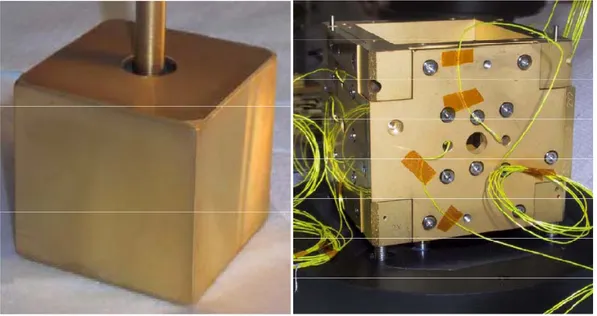
The test mass is the core element of the GRS, it is simply a 46 mm cube of gold‐platinum alloy with very low magnetic susceptibility (Figure 1‐10). The electrodes that surround the test mass are used for two purposes:
• To measure capacitively the displacements and the rotations of the test mass with respect to the spacecraft.
• To be able to apply forces and torques on the test mass in each degree of freedom. The box that contains the test mass and where the capacitor plates (electrodes) are placed is called test mass housing, its X axis is aligned with the telescope direction and its Z axis is normal to the spacecraft solar array.
12 Figure 1‐10: Test mass and electrode housing, Ref[1] The GRS features a total of 18 electrodes, 12 are intended for actuation purpose (green), 6 are the injection electrodes (red) used for sensing purpose. Note that in Figure 1‐12 the four electrodes on the z faces are intended as two. Figure 1‐11: GRS electrodes configuration, Ref[5]
Hence, 18 capacitances are defined between the TM and the electrodes and an additional capacitance between the test mass and the housing is taken into account.
Figure 1‐11 and 1‐12 show the electrode numbering and the relevant coordinates (note that in Figure 1‐12 the electrode 15 represents the electrodes 15 and 16, and the electrode 16 represents the electrodes 17 and 18).
13 Figure 1‐12: GRS electrodes numbering, Ref[5]
1.5 Contribution of This Work
• Implementation of the model of the Gravity Reference Sensor and the related actuation and sensing algorithms developed for LISA Pathfinder (LPF) in the LISA E2E Simulator. • Re‐parameterization according with the LISA GRS specifications of the GRS model, theactuation and the sensing algorithms.
• Development of an alternative actuation algorithm in science mode based on minimization of the actuation stiffness in order to reduce the parasitic effects involved in the test mass electrostatic suspension control. Simulation and validation by means of the LISA E2E Simulator.
• Analytical derivation of the actuation stiffness matrix in minimization of actuation stiffness approach. Analysis and validation of the results by means of the LISA E2E Simulator. Comparison with the same analysis done for LISA Pathfinder where a constant stiffness actuation approach is used.
• Analysis of the force and torque noises induced by the Front End Electronics (FEE) in minimization of actuation stiffness control approach. Comparison with the same analysis done for LISA Pathfinder in constant stiffness. • Analysis of some alternative Front End Electronics waveforms generation architectures in minimization of actuation stiffness.
1.6 Outline of the Thesis
This report has been divided in three parts, the first part constitutes a system‐level introduction to the following parts. In chapter 2, a brief description of the GRS functions is presented. In14
chapter 3, the main LISA operational modes are described and the GRS actuation strategies and the following conversion laws derived for LPF are presented. In chapter 4, the FEE architectures developed for LPF in two different operational modes are described.
The second part is focused on the implementation of the model of GRS in the LISA E2E Simulator. In chapter 5 the LISA E2E Simulator is briefly described and the mathematical model developed for the implementation of the GRS actuation in the Matlab‐Simulink environment is presented . Chapter 6 is focused on the problems connected with the parameterization of the GRS Model according with the LISA GRS specifications.
In the third part the effect of an alternative actuation strategy (stiffness minimization) in science mode is presented. In particular, in chapter 7, the actuation stiffness matrix is analytically derived and validated by means of the E2E Simulator and, in chapter 8, the noise induced by the FEE is derived and compared with the noise calculated in constant stiffness. In chapter 9 some possible alternative FEE architectures are illustrated. In chapter 10 the simulation results in minimization of stiffness control approach are presented. Finally, chapter 11 proposes a summary of the obtained results and suggests useful guidelines for future improvements.