Candidate:
dott. Vincenzo Lomonaco
Supervisor: prof. Davide Maltoni
School of Science
Master Degree in Computer Science
Academic year 2014-15 Session II
nature and the mutual positions of the beings that compose it, if this intellect were vast enough to submit the data to analysis, could condense into a single formula the movement of the greatest bodies of the universe and that of the lightest atom; for such an intellect nothing could be uncertain and the future just like the past would be present before its eyes.”
dott. Vincenzo Lomonaco
Negli ultimi anni, le tecniche di Deep Learning si sono dimostrate particolarmente utili ed efficaci nel risolvimento di una grande variet`a di problemi, sia nel contesto della vi-sione artificiale che in quello dell’ elaborazione del linguaggio naturale, raggiungendo e spesso superando lo stato dell’arte [1] [2] [3]. Il successo del deep learning sta rivoluzio-nando l’intero campo dell’ apprendimento automatico e del riconoscimento di forme avvalendosi di concetti importanti come l’ estrazione automatica delle caratteristiche ed apprendimento non supervisionato [4].
Tuttavia, nonostante il grande successo raggiunto sia in ambiti accademici che industri-ali, anche il deep learning ha cominciato a mostrare delle limitazioni intrinseche. Infatti, la comunit`a scientifica si domanda se queste tecniche costituiscano solo un sorta di ap-proccio statistico a forza bruta e se possano operare esclusivamente nell’ambito dell’ High Performance Computing con un enorme quantit`a di dati [5] [6]. Un’ altra ques-tione importante riguarda la possibilit`a di comprendere quanto questi algoritmi siano biologicamente ispirati e se possano scalare bene in termini di “intelligenza”.
L’ elaborato si focalizza sul tentativo di fornire nuovi spunti per la risoluzione di questi quesiti chiave nel contesto della visione artificiale e pi`u specificatamente del riconosci-mento di oggetti, un compito che `e stato completamente rivoluzionato dai recenti sviluppi nel campo.
Dal punto di vista pratico, nuovi spunti potranno emergere sulla base di un’ esaustiva comparazione di due algoritmi di deep learning molto differenti tra loro: Convolutional Neural Network (CNN) [7] e Hierarchical Temporal memory (HTM) [8]. Questi due algoritmi rappresentano due approcci molto differenti seppur all’interno della grande famiglia del deep learning, e costituiscono la scelta migliore per comprendere appieno punti di forza e debolezza reciproci.
a convoluzione sono state ben recepite ed accettate dalla comunit`a scientifica e, ad oggi, sono gi`a adoperate in grandi industrie tecnologiche del calibro di Google e Facebook per problemi come il riconoscimento del volto [9] e l’ auto-tagging di immagini [10].
L’algoritmo HTM, invece, `e principalmente conosciuto come un nuovo ed emergente paradigma computazionale biologicamente ispirato che si basa principalmente su tec-niche di apprendimento non supervisionate. Esso cerca di integrare pi`u indizi dalla comunit`a scientifica della neuroscienza computazionale per incorporare concetti come il tempo, il contesto e l’ attenzione nei processi di apprendimento che sono tipici del cervello umano.
In ultima analisi, la tesi si presuppone di dimostrare che in certi casi, con una quantit`a inferiore di dati, L’ algoritmo HTM pu`o risultare vantaggioso rispetto a quello CNN [11].
dott. Vincenzo Lomonaco
In recent years, Deep Learning techniques have shown to perform well on a large variety of problems both in Computer Vision and Natural Language Processing, reaching and often surpassing the state of the art on many tasks [1] [2] [3]. The rise of deep learning is also revolutionizing the entire field of Machine Learning and Pattern Recognition pushing forward the concepts of automatic feature extraction and unsupervised learning in general [4].
However, despite the strong success both in science and business, deep learning has its own limitations. It is often questioned if such techniques are only some kind of brute-force statistical approaches and if they can only work in the context of High Performance Computing with tons of data [5] [6]. Another important question is whether they are really biologically inspired, as claimed in certain cases, and if they can scale well in terms of “intelligence”.
The dissertation is focused on trying to answer these key questions in the context of Computer Vision and, in particular, Object Recognition, a task that has been heavily revolutionized by recent advances in the field.
Practically speaking, these answers are based on an exhaustive comparison between two, very different, deep learning techniques on the aforementioned task: Convolutional Neural Network (CNN) [7] and Hierarchical Temporal memory (HTM) [8]. They stand for two different approaches and points of view within the big hat of deep learning and are the best choices to understand and point out strengths and weaknesses of each of them.
CNN is considered one of the most classic and powerful supervised methods used today in machine learning and pattern recognition, especially in object recognition. CNNs
auto-tagging problems [10].
HTM, on the other hand, is known as a new emerging paradigm and a new meanly-unsupervised method, that is more biologically inspired. It tries to gain more insights from the computational neuroscience community in order to incorporate concepts like time, context and attention during the learning process which are typical of the human brain.
In the end, the thesis is supposed to prove that in certain cases, with a lower quantity of data, HTM can outperform CNN [11].
moments.
Giovanni Lomonaco, for helping me to develop my ideas on brain, learning and artificial intelligence.
Pierpaolo Del Coco, Ivan Heibi, Antonello Antonacci and many other fellow students, for helping me to develop my current skills through many years of projects, discussions, exams and fun.
Andrea Motisi, Ferdinando Termini and all the people from my student house, for giving me so much strength and comfort also outside the university spaces.
Matteo Ferrara and Federico Fucci, who helped me with the server configurations, their experience and pleasant company.
The many thinkers and friends, whose ideas and efforts have significantly contributed to shape my professional and human personality.
Sommario ii Abstract iv Acknowledgements vi Contents vii List of Figures ix List of Tables xi Abbreviations xii Introduction 1 1 Background 3 1.1 Machine Learning. . . 3
1.1.1 Categories and tasks . . . 4
1.2 Computer Vision . . . 5
1.2.1 Object recognition . . . 6
1.3 Artificial neural networks . . . 6
1.3.1 From neuron to perceptron . . . 7
1.3.2 Multilayer perceptron . . . 10
1.3.3 The back-propagation algorithm . . . 11
1.4 Deep Learning . . . 14
2 CNN: State-of-the-art in object recognition 16 2.1 Digital images and convolution operations . . . 16
2.1.1 One-to-one convolution . . . 17
2.1.2 Many-to-many convolution . . . 18
2.2 Unsupervised feature learning . . . 19
2.3 Downsampling . . . 20
2.4 CNN architecture . . . 23
2.5 CNN training . . . 24 vii
4 NORB-Sequences: A new benchmark for object recognition 39
4.1 The small NORB dataset . . . 39
4.1.1 Dataset details . . . 40
4.2 NORB-Sequences design . . . 41
4.3 Implementation . . . 43
4.4 Standard distribution . . . 48
4.5 KNN baseline: first experiments . . . 49
5 Comparing CNN and HTM: Experiments and results 52 5.1 Experiments design . . . 52
5.2 CNN implementation. . . 53
5.2.1 Theano . . . 54
5.2.2 Lenet7 in Theano. . . 55
5.3 HTM implementation . . . 63
5.4 Validation of the CNN implementation . . . 65
5.5 On NORB dataset . . . 69 5.5.1 Setup . . . 69 5.5.2 Results . . . 70 5.6 On NORB-Sequences. . . 72 5.6.1 Setup . . . 72 5.6.2 Results . . . 72
6 Conclusions and future work 76 6.1 Conclusions . . . 76
6.2 Future work . . . 77
1.1 Anatomy of a multipolar neuron [12].. . . 7
1.2 A graphical representation of the perceptron [13]. . . 8
1.3 Multilayer Perceptron commonly used architecture [14]. . . 11
1.4 Another Multilayer Perceptron architecture example [13]. . . 12
1.5 At every iteration, an error is associated to each perceptron to update the weights accordingly [13]. . . 13
2.1 Examples of a digital image representation and a 3x3 convolution matrix or filter [13]. . . 17
2.2 First step of a convolution performed on a 7x7 image and a 3x3 filter. . . 18
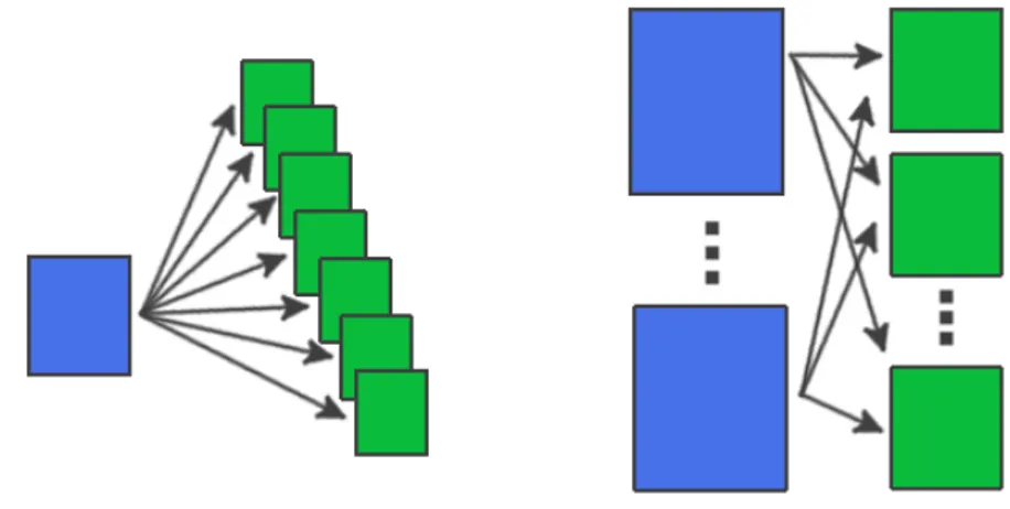
2.3 One-to-many and many-to-many convolution examples. . . 19
2.4 A convolution step performed with a perceptron. . . 20
2.5 Two imput images and one perceptron that operates as a filter. . . 21
2.6 Image chunking in a downsampling layer [13]. . . 22
2.7 General CNN architecture composed of a feature module and a neural network of n perceptron. . . 23
2.8 Layers alternation in a CNN features module. . . 23
2.9 A complete example of a CNN architecture with seven layer, or commonly called LeNet7 from the name of its author Y. LeCun. All the convolutions are many-to-many, i.e. each feature map has a perceptron that can be connected with two or more feature maps of the previous layer. . . 24
3.1 HTM hierarchical tree-shaped structure. An example architecture for processing 16x16 pixels images [11].. . . 31
3.2 a) Notation for message passing between HTM nodes. b) Graphical rep-resentation of the information processing within an intermediate node [15]. 32 4.1 The 50 object instances in the NORB dataset. The left side contains the training instances and the right side the testing instances for each of the 5 categories originally used in [16]. . . 41
4.2 Example sequence of ten images. . . 43
4.3 An header example contained in train configuration file. . . 44
4.4 An example sequence with its own header. . . 45
4.5 An header example contained in the test configuration file . . . 45
4.6 Sequences browser GUI. . . 46
4.7 A complete configuration file example. . . 47
4.8 KNN experiments accuracy results . . . 49
4.9 Explanatory example of how the KNN algorithm works. In this case, K is equal to one and the number of classes is two. . . 50
5.4 On the left jitter directions are esemplified, on the right an example of a jittered image is reported (the two images are overlapped). . . 67 5.5 Plotted accuracy results of a LeNet7 on different training size, with
jit-tered images or not. X coordinates are equispaced for an easier under-standing. . . 68 5.6 Averaged 5-fold accuracy comparation between CNN and HTM on
4.1 The different configuration files of the standard distribution prototype. . . 48 5.1 Accuracy results comparison among two different CNN architecture and
a NN baseline on different training size . . . 66 5.2 Training time comparison among two different CNN architecture on
dif-ferent training size . . . 67 5.3 Accuracy results of a LeNet7 on different training size, with jittered
im-ages or not. . . 68 5.4 Training time comparison between GPU and CPU implementation with
Theano . . . 69 5.5 Averaged accuracy results of a LeNet7 on different training size after a
5-fold cross-validation. . . 70 5.6 HTM averaged accuracy results on different training size after a 5-fold
cross-validation. Training times include unsupervised and HSR phases. . . 71 5.7 Accuracy results of the CNN trained on different training size and tested
on different test sets collected in the NORB-sequences benchmark. Note that the accuracy is high because the CNN is trained on all the instances of the five classes.. . . 73 5.8 Accuracy results of the CNN trained on 5 sequences of 20 images for each
class and tested on different test sets collected in the NORB-sequences benchmark. In this case eventually duplicated images are included in the training, validation and test sets. . . 73 5.9 Accuracy results of the CNN trained on different training size and tested
on different test sets collected in the NORB-sequences benchmark. Note that the accuracy is low because 50 different classes are considered (one for each instance). . . 74 5.10 Accuracy results of the HTM trained on different training size and tested
on different test sets collected in the NORB-sequences benchmark. In red, the accuracy results that are better than what reported for the CNN are highlighted. . . 74 5.11 Accuracy results of the HTM trained on different training size and tested
on different test sets collected in the NORB-sequences benchmark. 50 different classes are considered. In red, the accuracy results that are better than what reported for the CNN are highlighted. . . 75
CUDA Compute Unified Device Architecture
CV Computer Vision
DL Deep Learing
GIF Graphics Interchange Format
HSR HTM Supervised Refinement
HTM Hierarchical Temporal Memory
JPEG Joint Photographic Experts Group
KNN K-Nearest Neighbor
MHWA Multi-stage Hubel-Wiesel Architectures
ML Machine Learing
MLP Multy Layer Perceptron
NN Neural Network
NORB New York Object Recognition Benchmark
PNG Portable Network Graphics
PNS Peripheral Neurvous System
RGB Red Green and Blue
RL Reinforcement Learning
the chapter we have written together in the wonderful book of life.
in the field of machine learning, a regained interest in these matters seems to lead the research community all over the world [18]. A catalyzing factor is, for sure, the unlock of generalized features learning methods, i.e. the ability of automatically discriminate class features without any domain-specific instructions [4]. This is thought to be at the heart of intelligence, and it is concretely helping many business applications. This new machine learning trend that comes with the name of Deep learning, is deeply changing the way machine learning was performed, generally with hand-crafted extraction of salient features [19]. The computer vision community, for example, can work out now, for the first time, methods that are dealing directly with raw images data. Actually, most of the insights that are conducting recent research progress, are dated back in the last century. However, only recent advances in technology (computational speed) and further mathematical tricks have enabled the real usefulness and effectiveness of these approaches.
In fact, deep learning techniques are incredibly computationally intensive and they need a huge quantity of data to work well. Moreover, they are criticized to be too focused on certain mathematical aspects and to ignore fundamental principles of intelligence. A consistent part of the scientific community is working hard to answer these questions. The current dissertation fits exactly on this research track and tries to compare two deep learning algorithms (CNN and HTM) in a computer vision context, specifically in object recognition. It has two main goals. Firstly, pushing object recognition research towards images sequences or video analysis, and secondly proving that with a lower quantity of data HTM can outperform CNN in terms of accuracy while remaining comparable in terms of training times. In Chapter 1 a brief background about machine learning and
artificial neural networks will be covered. In chapter 2 and 3, the two algorithms will be explained in great details. In chapter4, a new benchmark for image sequences will be introduced and in chapter 5, experiments results will be reported. Eventually, in chapter 6conclusions will be drawn and future work directions suggested.
sense works so well not because it is an approximation of logic; logic is only a small part of our great accumulation of different, useful ways to chain things together.”
– prof. Marvin Lee Minsky, The Society of Mind (1987)
In this chapter a brief background about machine learning and artificial neural networks is provided. In the following sections the reader will be introduced to the main concepts behind the work carried out in this dissertation, even with the help of strict mathematical notations when required.
1.1
Machine Learning
Learning is a very interesting and articulated phenomenon. Learning processes include the acquisition of new declarative knowledge, the development of motor and cognitive skills through instruction or practice, the organization of new knowledge into general, effective representations, and the discovery of new facts and theories through observation and experimentations. Since the birth of computing, researchers have been striving to implant such capabilities in computers. Solving this problem has been, and still remains, one of the most challenging and fascinating long-term goals in artificial intelligence. The study of computer modeling of learning processes in their multiple manifestations constitutes the subject matter of machine learning.
In 1959, Arthur Samuel defined machine learning as a “Field of study that gives com-puters the ability to learn without being explicitly programmed ” [20].
Tom M. Mitchell provided a widely quoted, more formal definition: “A computer program is said to learn from experience E with respect to some class of tasks T and performance measure P, if its performance at tasks in T, as measured by P, improves with experience E ” [21].
This definition is notable because it defines machine learning in fundamentally oper-ational terms rather than cognitive ones, thus following Alan Turing’s proposal in his paper Computing Machinery and Intelligence that the question “Can machines think?” be replaced with the question “Can machines do what we (as thinking entities) can do?” [22]
1.1.1 Categories and tasks
Usually, machine learning tasks are classified into three broad categories. These depend on the nature of the learning “signal” or “feedback” available to a learning system: [17]
• Supervised learning: Is the machine learning approach of inferring a function from supervised training data. The training data consist of a set of training ex-amples i.e. pairs consisting of an input object (typically a vector) and a desired output value (also called the supervisory signal). A supervised learning algorithm analyzes the training data and produces an inferred function, which can generalize from the training data to unseen situations in a “reasonable” way.
• Unsupervised learning: Closely related to pattern recognition, unsupervised learning is about analyzing data and looking for patterns. It is an extremely powerful tool for identifying structure in data. Unsupervised learning can be a goal in itself or a means towards an end.
• Reinforcement learning: Is learning by interacting with an environment. An RL agent learns from the consequences of its actions, rather than from being explic-itly taught and it selects its actions on basis of its past experiences (exploitation) and also by new choices (exploration), which is essentially trial and error learning. The reinforcement signal that the RL-agent receives is a numerical reward, which encodes the success of an action’s outcome, and the agent seeks to learn to select actions that maximize the accumulated reward over time.
Between supervised and unsupervised learning another category of learning methods can be found. It is called Semi-supervised learning and it is used in the presence of an
human teachers. It also uses guidance mechanisms such as active learning, maturation, motor synergies, and imitation.
Another categorization of machine learning tasks arises considering the desired output of a machine-learned system: [23]
• In classification, inputs are divided into two or more classes, and the learner must produce a model that assigns unseen input patterns to one or more of these classes (fuzzy classification). This is typically tackled in a supervised way. Spam filtering is an example of classification, where the inputs are email (or other) messages and the classes are “spam” and “not spam”.
• In regression, which is also a supervised problem, the outputs are continuous rather than discrete.
• In clustering, a set of input patters have to be divided into groups. Unlike in classification, the groups are not known beforehand, making this typically an unsupervised task. Topic modeling is a related problem, where a program is given a list of human language documents and is asked to find out which documents cover similar topics.
• Density estimation finds the distribution of input patterns in some space. • Dimensionality reduction simplifies inputs by mapping them into a
lower-dimensional space.
1.2
Computer Vision
Computer vision is a field which collects methods for acquiring, processing, analyzing, and understanding images and, in general, high-dimensional data from the real world. The aim of the discipline is to elaborate these data to produce numerical or symbolic information in the forms of decisions [24]. A fundamental idea that has always stood
behind this field has been to duplicate the abilities of human vision by electronically perceiving and understanding an image [25]. This image understanding can be seen as the disentangling of symbolic information from image data using models constructed with the aid of geometry, physics, statistics, and learning theory [26]. Computer vision has also been defined as the enterprise of automating and integrating a wide range of processes and representations for vision perception.
Being computer vision a scientific discipline, it is concerned with the theory behind artificial systems extracting information from images. The image data can take many forms, such as image sequences, views from multiple cameras, or multi-dimensional data from a medical scanner. From a technological point of view, computer vision seeks to apply its theories and models to the construction of computer vision systems.
Sub-fields of computer vision include object recognition, scene understanding, video tracking, event detection, object pose estimation, learning, indexing, motion estimation, and image restoration.
1.2.1 Object recognition
Object recognition is the task within computer vision which is concerned with the finding and identification of objects in images or video sequences. Humans are able to recognize a multitude of objects without much effort, despite the fact that the objects in the images may vary significantly due to different view points, many different sizes and scales, lighting conditions and poses. Objects can even be recognized when the view is partially obstructed. This task is still a challenge for computer vision systems. Many approaches to the task have been implemented over multiple decades. In this dissertation, this task will be confronted in-depth.
1.3
Artificial neural networks
In machine learning, artificial neural networks (ANNs) are a family of statistical learning models inspired by biological neural networks (common in the brains of many mammals) [17]. They can be used to estimate or approximate functions that can depend on a large number of inputs and are generally unknown. Artificial neural networks are generally presented as systems of interconnected “neurons” which send messages to each other. Each of their connection has a numeric weight that can be tuned based on experience, making neural nets adaptive to inputs and capable of learning [27].
1.3.1 From neuron to perceptron
A neuron, also known as “neurone” or “nerve cell”, is an electrically excitable cell that processes and transmits information through electrical and chemical signals [28]. These signals between neurons occur via synapses, specialized connections with other cells. Neurons can connect to each other to form neural networks. Neurons are the key components of the brain and spinal cord of the central nervous system (CNS), and of the ganglia of the peripheral nervous system (PNS). Specialized types of neurons include: sensory neurons which respond to touch, sound, light and all other stimuli affecting the cells of the sensory organs that then send signals to the spinal cord and brain, motor neurons that receive signals from the brain and spinal cord to cause muscle contractions and affect glandular outputs, and interneurons which connect neurons among each other within the same region of the brain or the spinal cord.
A typical neuron consists of a cell body (soma), dendrites, and an axon. The term neurite is used to describe either a dendrite or an axon, particularly in its undifferentiated stage. Dendrites are thin structures arising from the cell body, often extending for hundreds of micrometres and branching multiple times, giving rise to a complex “dendritic tree”. An axon is a special cellular extension that arises from the cell body at a site called the axon hillock and travels for a distance, as far as 1 meter in humans or even more in other species. The cell body of a neuron frequently brings about multiple dendrites, but never more than one axon, although the axon may branch hundreds of times before it terminates. To the majority of synapses, signals are sent from the axon of one neuron to a dendrite of another.
Figure 1.2: A graphical representation of the perceptron [13].
The perceptron is the mathematical abstraction of a neuron and a binary classifier that combined with other counterparts can lead to great results in pattern recognition [29]. A perceptron receives an input vector x consisting of n elements. The linear combination c of the vector input x and a weight vector w is called action potential. The inputs of the perceptron represent signals collected from dendrites, while the weights represent the signal attenuation exercised by the neuron. However, unlike real neurons, the perceptron can also amplify its input. The threshold of a neuron is represented by b, which is then added to c. Finally, the result of this sum is passed to the activation function f and y is its return value. In fig. 1.2 a graphical explanation of the perceptron is provided. To explain how to interpret the value of y, considering that, for example, there are only two classes to distinguish, a value of y less or equal than 0 then could indicate that the input belongs to the first class (-1), and accordingly, a value of y greater than 0 could indicate that the input belongs to the second class (1).
The weights w1, w2, w3, . . . , wn, the threshold b and the function f are the fundamental
characteristics that distinguish a perceptron from another. The activation function is chosen at the design time depending on the data set (e.g. set of patterns in the training
• w it is the vector composed of all weights associated with the input of the percep-tron.
• b is the threshold associated with the perceptron. • m is the number of elements in the training set. • f is the activation function of choice.
• xj is the j-th example (each example is a vector) of the training set.
• zj is the desired result that should give the perceptron when it receives ad input
the j-th sample of the training set.
• n is the number of weights, one speaks then of the number of elements in the vector w.
The formula 1.1 can be suitably simplified considering b as a weight within w (w0 = b)
and associating to it an input x0 = 1. As a result the following equation is obtained:
E(w) = m X j=1 Txj(w) (1.2) Txj(w) = 1 2(f ( n X i=0 (wi, xji)) − zj)2 (1.3)
Hence, after having provided the error equations, the objective is to find the combination of values for w that minimizes E(w). For this purpose a minimization method which starts from a random solution can be applied. Indeed, using a gradient descent technique implemented as an iterative method it is possible to get closer and closer to the minimum point that corresponds to the solution of the problem. Frank Rosenblatt, who invented the perceptron, showed that the process just discussed above can be obtained with the following iterative steps:
In the equation:
• wj is the weight vector at step j.
• α is the learning rate, which is the displacement step to minimize the error; If it is too large it can make impossible to reach the minimum, while if it is too small it can greatly slow down the convergence.
• yj is the output of the perceptron when it processes input xj.
• (zj − yj)f0(wjxj) can be seen as the mistake of the perceptron prosessing the
pattern xj.
• −(zj− yj)f0(wjxj)xj is the gradient of Txj calculated on wj.
The minimum of E can be achieved by repeating the procedure in1.4starting each time from the last vector of the weights obtained from the previous computation.
Despite its mathematical elegance and due to its inherent simplicity, a perceptron can only solve binary classification problems. Moreover, it can perform only a linear classi-fication, which can not be accurate when patterns are not linearly separable. In spite of everything, the perceptron is the necessary building block of the entire work carried out and discussed in this dissertation as well as a critical invention for the field of ma-chine learning. Of course, there are many other mama-chine learning techniques that do not rely on neural networks abstractions, but there is no interest in discussing them in this context.
1.3.2 Multilayer perceptron
In the light of the strong limitations of the perceptron, trying to link multiple units to create a larger structure appears natural. The first example of an artificial neural network was called multilayer perceptron (MLP) [30]. A multilayer perceptron can clas-sify non linearly separable patterns and works well even when there are more than two classes. Theoretically perceptrons can be combined at will, but more than thirty years of research effort have established commonly adopted rules for simple feed-forward net-works in order to build efficient and effective architectures for solving useful problems in pattern recognition:
• A MLP should have one or more input perceptrons, i.e. perceptrons that receive as input the original pattern which is not coming from other perceptrons.
• A MLP should have as many output perceptrons as classes (each of these represents a class), where an output perceptron is a simple unit that does not have exit connections.
Figure 1.3: Multilayer Perceptron commonly used architecture [14].
• Given a pattern p as input, a MLP should associate p to the class represented by the output perceptron computing the higher value among its peers.
• In a MLP, the set of input and output perceptrons should not be necessarily disjoint;
• In a MLP, all the perceptrons should share the same activation function; • In a MLP, connections among perceptrons should not be cyclic.
In figure1.3is shown the most used MLP architecture in machine learning. it is a three-layer architecture composed of an input three-layer, a hidden three-layer and an output three-layer. The input layer is not composed of real perceptrons but simple propagators which provide the same input to all the perceptrons of the hidden layer. On the other hand, in the hidden layer each perceptron is connected to each perceptron in the output layer. Finally, the output layer has no output connections. Broadly speaking, the network showed in fig. 1.3, is a feed-forward artificial neural network in which perceptrons take their input only from the previous layer, and send their output only to the next layer. To train a neural network a powerful technique called back-propagation can be used [31]. This algorithm, unknown until the ’80s, can adjust the weights of the network propagating the error backwards (starting from the output layer). In the following paragraph, this technique is described in detail. Unlike the perceptron, artificial neural networks are good classifiers even if it is worth pointing out that they are very different from their biological counterparts.
1.3.3 The back-propagation algorithm
The back-propagation technique, requires to consider for each iteration a new training pattern x. Assuming that the output of the hidden layer are q1, q2, q3, . . . , qm, it is
Figure 1.4: Another Multilayer Perceptron architecture example [13].
qi= f (hix) ∀i = 1, . . . , m (1.5)
Then, y1, y2, y3, . . . , yn, the output of the MLP, can be computed as follows:
yi= f (wiq) ∀i = 1, . . . , n (1.6)
Where:
• wi is the weights vector associated with the i-th perceptron in the output layer;
• hi is the weight vector associated with the i-th perceptron in the hidden layer
• f is the activation function.
The last square error on x of the MLP can be calculated as follows:
Tx= 1 2 n X i=1 (zi− yi)2 (1.7)
In the above equation, zi is the exact result the ith output perceptron should produce
and which can be retrieved from the training set. As for the perceptron, we would like to minimize the error by finding the right combination of values for wi for i = 1, . . . , n
and hj for j = 1, . . . , m. Also in this case a gradient descent technique can be applied
in order to minimize the error function. For the minimization we start calculating the error from the output layer:
Figure 1.5: At every iteration, an error is associated to each perceptron to update the weights accordingly [13].
ei= (zi− yi)f0(wiq) ∀i ∈ {1, . . . , n} (1.8)
Then the error can be propagated backward, based on that computed on the output layer: ri = f0(hix) n X k=i ekwki ∀i ∈ {1, . . . , m} (1.9)
In this case we are considering a neural network with just one hidden layer, but the back-propagation can be easily extended to any type of network by repeating the computation shown in 1.9 by treating the next hidden layer as if it were the output layer. After the error back-propagation the input weights of the output perceptrons can be updated as follows:
wi = wi+ α · ei· q ∀i ∈ {1, . . . , n} (1.10)
And the input weights of the hidden layer can be adjusted as follows:
hi = hi+ α · ri· x ∀i ∈ {1, . . . , m} (1.11)
With the last two equations, just a single step ahead (with a learning rate of α) in the opposite direction to the gradient of Tx (computed on the previous configuration of
weights) has been made. Repeating this procedure for each pattern in the training set completes the back-propagation. Now let’s consider the corresponding pseudo-code:
Algorithm 1 back-propagation algorithm
1: procedure Back–Propagation 2: for each input pattern x do
3: forward propagation
4: compute error for each output perceptron
5: for i = K to 1 do //with K number of hidden layer
6: back-propagate error on the hidden layer i
7: end for
8: update weights of the output perceptrons
9: for i = K to 1 do
10: update weights of the hidden layer i
11: end for
12: end for
13: end procedure
Moreover, to minimize the error of all the examples, the back-propagation is repeated several times always starting from the last configuration of weights computed in the previous iteration. The training ends after a predetermined number of iteration or if the error committed by the network does not exceed a certain threshold. It is worth saying that using a constant learning rate could not be that good and we may want to decrease it at each iteration to be more and more accurate as the training goes on.
1.4
Deep Learning
Deep learning (deep machine learning, or deep structured learning, or hierarchical learn-ing, or sometimes DL) is a branch of machine learning which comprises a set of algorithms attempting to model high-level abstractions in data through model architectures with complex structures or otherwise, composed of multiple non-linear transformations. [32] Deep learning is part of a broader family of machine learning methods based on learning representations of data. An observation (like an image, for example) can be coded in many ways such as a vector of intensity values, or more abstractly as a set of edges, regions of particular shape, etc... Some representations make it easier to learn tasks (e.g., face recognition or facial expression recognition) from examples.
The most important and characterizing feature of deep learning is the depth of the net-work. Until a few years ago, it was thought that an MLP with a single hidden layer would have been sufficient for almost any complex task. With the increasing amounts of data and computing power now available, the advantage of building deep neural net-works with a large number of layer (up to 10 or even greater) has been recognized. As already mentioned, another important feature of deep learning the ability of replac-ing handcrafted features with efficient algorithms for unsupervised or semi-supervised feature learning and hierarchical feature extraction.
to fields like computer vision, automatic speech recognition, natural language processing, audio recognition and bioinformatics where they have been shown to produce state-of-the-art results on various tasks. Besides, deep learning is often regarded as buzzword, or a simple rebranding of neural networks [34].
CNN: State-of-the-art in object
recognition
“If we were magically shrunk and put into someone’s brain while she was think-ing, we would see all the pumps, pistons, gears and levers working away, and we would be able to describe their workings completely, in mechanical terms, thereby completely describing the thought processes of the brain. But that de-scription would nowhere contain any mention of thought! It would contain nothing but descriptions of pumps, pistons, levers!”
– G. W. Leibniz (1646–1716)
The current chapter describes in details the Convolutional Neural Network (CNN) ap-proach to pattern recognition starting from the basic concepts of convolution and arti-ficial neural network. The algorithm is introduced in the context of object recognition, focus of this dissertation, even if these networks can be conveniently used on patterns of any type.
2.1
Digital images and convolution operations
A digital image can be defined as the numerical representation of a real image. This representation can be coded as a vector or a bitmap (raster). In the first case it describes the primitive elements (lines or polygons) which compose the image, in the second case the image is composed of a matrix of points, called pixels. Their color is defined by one or more numerical values. In coloured bitmap images the color is stored as level of intensity of the basic colors, for example in the RGB model there are three colors: red,
Figure 2.1: Examples of a digital image representation and a 3x3 convolution matrix or filter [13].
green and blue. In grayscale (improperly called black and white) bitmap images the value indicates different gray intensities ranging from black to white. The images that are further elaborated in this dissertation are grayscale bitmap images. The number of colors or possible gray levels (depth) depends on the amount of bits used to code them: an image with 1 bit per pixel will have a maximum of two possible combinations (0 and 1) and thus may represent only two colors, images with 4 bits per pixel can represent up to 16 colors or 16 levels of gray, an image with 8-bit per pixel can represent 256 colors or gray levels, and so on. Bitmap images can be stored in different formats often based on a compression algorithm. The algorithm can be lossy (JPEG) or lossless, i.e. without loss (GIF, PNG). This type of images is generated by a wide variety of acquisition devices, such as scanners, digital cameras, webcams, but also by radar and electronic microscopes.
2.1.1 One-to-one convolution
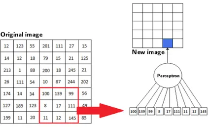
The convolution [24] is an operation that is performed on a mono-color bitmap image for emphasizing some of its features. In order to do so, a digital image and a convolution matrix are needed, consider the fig. 2.2. The convolution matrix is also called filter. A filter can be thought as a sliding window moving across the original image. At every shift it produces a new value, this value is obtained by summing all the products between the filter elements and the corresponding pixels. The values obtained from all the possible placements of the filter above the image are inserted in an orderly fashion in a new image. With a convolution is therefore obtained an image that highlights the characteristics enhanced by the filter used. Then, as regards the size of the new image we have:
Figure 2.2: First step of a convolution performed on a 7x7 image and a 3x3 filter.
bn= bv− bf+ 1 and hn= hv− hf+ 1 (2.1)
where:
• bn and hn are respectively the width and the height of new image resulting from
the convolution;
• bv and hv are respectively the width and the height of the original image;
• bf and hf are respectively the width and the height of the filter used.
In computer vision, several filters are often used and each of them has a particular purpose. The more popular are:
• Sobel filters: generally used to highlight edges; • Gaussian filters: generally used to remove noise;
• High-pass filter : generally used to increase image details;
• Emboss filter : generally used to accentuate brightness differences.
The convolution operation is at the heart of convolutional neural networks where filters are automatically learned in an unsupervised fashion during the training phase.
2.1.2 Many-to-many convolution
Until now, we have only discussed one-to-one convolutions that take in input a single image and return a single image as the output. Actually, different kind of convolutions
computational time increases sharply with the rise of the connections.
Figure 2.3: One-to-many and many-to-many convolution examples.
2.2
Unsupervised feature learning
Considering the simplest case, a step of convolution can be expressed with the following formula:
c = X
∀(i,j)∈S
Fi,j· Si,j (2.2)
where:
• c is the result of the convolution step convolution; • S is the considered sub-image;
• Fi,j is the element of row i and column j of the filter;
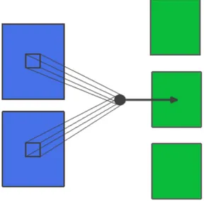
Figure 2.4: A convolution step performed with a perceptron.
Now, considering f as an arbitrary activation function and b as a bias, if we substitute the result of the convolution step c with y and we calculate y as follows:
y = f (c + b) (2.3)
Then we end up with a computation that is pretty similar to what described in the pre-ceding chapter regarding the perceptron. This is commonly referred to as a convolution performed with a perceptron where the weights of the former are the same of the filter. In a convolutional neural network the key element is the convolutional layer, or a module that performs many-to-many convolutions with many perceptrons. in this module, each output image has an associated perceptron that takes input from all the related images at every step of convolution. A convolutional layer has therefore a set of perceptrons and their training leads to the ideal filters depending on the cost function that is minimized through the back-propagation algorithm. In a convolutional layer, it is also possible to decrease the computational complexity and the output size by applying the filters every s pixels (where s is called stride). This is generally not recommended as it compromises the quality of the output.
2.3
Downsampling
In convolutional neural networks another important module called subsampling layer [32] exists: its main task is to carry out a reduction of the input images size in order to give the algorithm more invariance and robustness. A subsampling layer receives n input images, and provides n output; The images to be reduced are divided into blocks
Figure 2.5: Two imput images and one perceptron that operates as a filter.
that have all the same size, then, each block is mapped to a single pixel in the following way:
y = f ( X
∀(i,j)∈B
Bi,j· w + b) (2.4)
where:
• y is the result of the subsampling step; • f is the activation function;
• B is the block considered in the input image;
• Bi,j is the value of the pixel (i, j) within the block B;
• w is the adjustment coefficient; • b is the threshold;
The computation performed on an input image from a subsample layer is made by a per-ceptron that has all equal weights (threshold excluded). Hence, training n perper-ceptrons is sufficient to generate 2n parameters.
A subsample layer is less powerful than a convolutional layer. In fact, as previously pointed out, the higher is the number of trainable parameters the higher is the discre-tionary capacity of our network. Then, why not using only convolutional layers? There are three main reasons:
2. A subsampling layer performs its tasks more quickly than a convolutional layer due to a smaller number of steps and products;
3. The subsample layer allow CNN to tolerate translations and rotations among the input patterns. In practice, a single subsampling layer is not enough, but it has been seen that an alternation of feature extraction and subsampling layers can handle different types of invariance which a sequence of only convolutional layers can not manage.
It is also possible to modify a subsampling layer in order to divide the input images into overlapping blocks. Of course, this configuration can slow down the reduction process. Indeed, depending on the task, the temporal aspect could be extremely important both in the training and the test phases that might have to take place within few milliseconds. Sometimes even simpler downsampling layer can be used to speed-up the training. A great example of this approach is the so called max-pooling layer. In this layer only the following operation are performed:
• c1 is computed as the max value among the pixels of the block;
• c2 is obtained summing c1 with his bias;
• resulting pixel is obtained computing the activation function on c2
Figure 2.6: Image chunking in a downsampling layer [13].
In a CNN each subsampling layer can be replaced with a pooling layer. A max-pooling layer has less parameters to train due to the elimination of the adjustment coefficients. With the parameters reduction more speed is obtained during the training phase, but often with lower degree of learning.
that generates the results. The neural network is composed of n perceptron (as many as the classes) all both input and output. The feature module, instead, usually consists of a convolutional layer followed by zero, one or more pairs [subsampling layer, convolutional layer]. Hence, it has an odd number of sub-modules where the first and the last are convolutional layers. The last array of features is the result of the last convolutional layer where the input images are reduced to single values.
Figure 2.7: General CNN architecture composed of a feature module and a neural network of n perceptron.
If k is the number of layers in the CNN, it can be called a k-CNN or simpler, a CNN with k layers. In theory, the higher is k, the greater is the degree of learning of the network. However in practice, too many layers can create convergence problems during the training. To train a CNN the classic supervised approach based on back-propagation is used. This approach allows the network to learn how to discern a pattern from another based on the training set. In CNNs the sigmoidal function is commonly used as the activation function of all the layers (including the neural network).
In this section a general definition of a convolutional neural network has been provided. However, there are many variants depending on the task:
• CNN without final neural network;
• CNN with a final neural network with one or more hidden layers; • CNN with an even number of layers in their features module. • CNN with only convolutional layers.
In the dissertation we will continue to talk about CNNs referring to their general def-inition, even if it is important to understand that there are many researchers who can call with the same right convolutional neural networks slightly different architectures.
Figure 2.9: A complete example of a CNN architecture with seven layer, or commonly called LeNet7 from the name of its author Y. LeCun. All the convolutions are many-to-many, i.e. each feature map has a perceptron that can be connected with two or
more feature maps of the previous layer.
2.5
CNN training
A CNN is trained using the propagation algorithm already discussed in the back-ground chapter. Specifically, the neural network is trained using formulas1.8and 1.10. To train the generic module l it is important to consider the following one. If the layer l + 1 is the final neural network then we calculate the error as follows:
σlj(0, 0) = f0(alj(0, 0)) n X k=1 (ekwk,j) (2.5) where:
module l;
If, instead, the module l + 1 is a convolutional layer the error is calculated as follows:
σjl(x, y) = f0(alj(x, y)) X k∈Kl j X ∀(u,v)∈wl+1 k,j (σkl+1(x − u, y − v)wk,jl+1(u, v)) (2.6) where: • σl
j(x, y) is the error of the jth image if the module l, on the pixel with coordinates
(x, y) (if x < 0 or y < 0 then σjl(x, y) is equal to zero) • al
j(x, y) is the value passed to f in order to obtain the value of the pixel with
coordinates (x, y) of the jth image of the module l; • Kl
j is the set of indexes of the l + 1 module images connected with the jth image
of the module l;
• wl+1k,j(u, v) is the value of column u and row v of the filter associated to the con-nection between the image k of the module l + 1 and the image j of the module l;
Again, if the module l + 1 is a subsampling layer the error is calculated as follows:
σjl(x, y) = f0(alj(x, y))σl+1j (bx/Sxc, by/Syc)wl+1j (2.7)
where:
• Sx is the width of the blocks in which the images are divided; • Sy is the height of the blocks in which the images are divided;
Lastly, if the module l + 1 is a max-pooling layer:
σjl(x, y) =
0 if ylj(x, y) is not a local max
f0(alj(x, y))σjl+1(bx/Sxc, by/Syc) otherwise
(2.8)
where ylj(x, y) stands for the value of the pixel with coordinates (x, y) in the jth image of the module l.
Once errors are calculated we need to update the weights accordingly. If the module l is a convolutional layer then:
∆wj,il (u, v) = α X
∀(x,y)∈σl j
(σlj(x, y)yil−1(x + u, y + v)) (2.9)
where α is the learning rate. If, instead, the module l is a subsampling layer:
∆wjl = α X ∀(x,y)∈σl j Sx−1 X c=0 Sy−1 X r=0 (yil−1(x · Sx+ c, y · Sy+ r)) (2.10)
Having computed the gradient, the weights can be updated according to the different type of module as follows. If the module l is a convolutional layer:
wi,jl = wi,jl + ∆wlj,i(u, v) (2.11)
If, instead, the module l is a subsampling layer:
wjl = wlj+ ∆wlj (2.12)
With regard to the thresholds, they can be updated as follows:
blj = blj+ α X
∀(x,y)∈σl j
(σjl(x, y)) (2.13)
So far we have considered a single update of the weights. Repeating this procedure for each pattern in the training set completes the back-propagation. Consider the corre-sponding pseudo-code:
11: update weights of the module i
12: end if
13: update the thresholds of the module i
14: end for
15: end for
16: end procedure
As a final consideration let us consider the formula 2.8. If the layer l + 1 is a max-pool layer, then the total error for the images of the module l is small compared to the others. Hence the max-pool layer can accelerate the training not only for the smaller number of of parameters, but also because the initial error is lower.
HTM: A new bio-inspired
approach for Deep Learning
“Prediction is not just one of the things your brain does. It is the primary function of the neo-cortex, and the foundation of intelligence.”
– Jeffrey Hawkins, Redwood Center for Theoretical Neuroscience
The current chapter describes briefly the Hierarchical Temporal Memory (HTM) ap-proach to pattern recognition starting from its basic concepts. A comprehensive de-scription of HTM architecture and learning algorithms is provided in [11].
3.1
Biological inspiration
Since its early days, artificial intelligence has always been conditioned by its biological counterpart. Even if, first artificial neural networks had very little in common with biological ones, after a deeper understanding of the human visual system, multi-stage Hubel-Wiesel architectures (MHWA) [33] [36] arose, and deep learning sprouted. These kind of architectures base their success on the ability of automatically discovering salient and discriminative features in any pattern. However, they still rely fundamentally on back-propagation, a statistical algorithm that is not exactly biologically inspired. HTM tries to integrate more key elements from biological learning systems like the human brain. Additionally, comparing high-level structures and functionality of the neocortex with HTM is most appropriate. HTM attempts to implement the functionality that is characteristic of a hierarchically related group of cortical regions in the neocortex. A region of the neocortex corresponds to one or more levels in the HTM hierarchy, while
engineering and intuitions. In spite of its recent development it could help managing invariance, which is a pivotal issue in computer vision and pattern recognition. Thus, some important properties can be exploited:
• The use of time as supervisor. Since minor intra-class variations of a pattern can result in a substantially different spatial representation (e.g., in term of pixel in-tensities), huge efforts have been done to develop variation-tolerant metrics (e.g., tangent distance [39]) or invariant feature extraction techniques (e.g., SIFT [40]). However, until now, positive outcomes have been achieved only for specific prob-lems. HTM takes advantage of time continuity to assert that two representations, even if spatially dissimilar, originate from the same object if they come close in time. This concept, which lies at the basis of slow feature analysis [41], is simple but extremely powerful because it is applicable to any form of invariance (i.e., ge-ometry, pose, lighting). It also enables unsupervised learning: labels are provided by time.
• Hierarchical organization. Lately, a great deal of studies furnished theoretical support to the advantages of hierarchical systems in learning invariant represen-tations [33] [42]. Just like the human brain, HTM employs a hierarchy of levels to decompose object recognition complexity: at low levels the network learns basic features, used as building blocks at higher levels to form representations of in-creasing complexity. These building blocks are crucial as well for efficient coding and generalization because through their combination, HTM can even encode new objects which have never seen before.
• Top down and bottom-up information flow. In MHWA information typically goes only one-way from lower levels to upper levels. In the human cortex, both feed-forward and feed-back messages are steadily exchanged between different regions. The precise role of feed-back messages is still a heated debate, but neuroscien-tists agrees on their fundamental support in the perception of non-trivial patterns
[43]. Memory-prediction theory assumes that feed-back messages from higher lev-els bring contextual information that can bias the behavior of lower levlev-els. This is crucial to deal with uncertainty: if a node of a given level has to process an ambiguous pattern, its decision could be better taken with the presence of insights from upper levels, whose nodes are probably aware of contextual information the network is operating in (for example, if one step back in time we were recognizing a person, probably we are still processing a crowed scene).
• Bayesian probabilistic formulation. When uncertainty is the central issue, it is often better to take probabilistic choices rather than binary ones. In light of this, the state of HTM nodes is encoded in probabilistic terms and Bayesian theory is widely used to process information. HTM can be seen as a Bayesian Network where Bayesian Belief propagation equations are adopted to let information flow across the hierarchy [44]. This formulation is mathematically elegant and allows to solve practical hurdles such as value normalization and threshold selection.
Deepening into details, an HTM has a hierarchical tree structure. The tree is built up by nlevels levels (or layers), each composed of one or more nodes. A node in one level
is bidirectionally connected to one or more nodes in the level above and the number of nodes in each level decreases as the hierarchy is ascended. The lowest level L0, is the
input level and the highest level, nlevels−1, which usually contains only one node, is the
output level. Those levels and nodes that exist in between the input and output levels are called intermediate. When an HTM is exploited for visual inference, as is the case in this dissertation, the input level typically has a retinotopic mapping of the input. Each input node is connected to one pixel of the input image and spatially close pixels are connected to spatially close nodes. Refer to fig. 3.1for a graphical example of an HTM.
3.2.1 Information Flow
As already mentioned, in an HTM there is a bidirectional information flow. Belief propagation is used to send messages and information both up (feed-forward) and down (feedback) the hierarchy as new evidence is presented to the network. The notation used here for belief propagation (fig. 3.2.a) closely follows Pearl [44] and is adapted to HTMs by George [38]:
• Evidence that comes from below is denoted e−. In visual inference this corresponds to an image or video frame presented to level L0 of the network.
Figure 3.1: HTM hierarchical tree-shaped structure. An example architecture for processing 16x16 pixels images [11].
• Evidence coming from the top is denoted e+ and can be seen as contextual
infor-mation. This can for instance come from another sensor modality or the absolute knowledge of the supervisor training the network.
• Feed-forward messages sent up the hierarchy are denoted λ and feedback messages flowing down are denoted π.
• Messages entering and leaving a node from below are denoted λ− and π− respec-tively, relative to that node. Following the same notation as for the evidence, messages entering and leaving a node from above are denoted λ+ and π+.
When an HTM is meant as a classifier, the feed-forward message of the output node is the posterior probability that the input e− belongs to one of the problem classes. This posterior is denoted P (wi|e−) where wi is one of nw classes.
3.2.2 Internal Node Structure and Pre-training
Since the input level does not need any training and it just forwards the input, HTM training is performed level by level, starting from the first intermediate level. Interme-diate levels training is unsupervised and the output level training is supervised. For a detailed description, including algorithm pseudocode, the reader should refer to [11]. For
Figure 3.2: a) Notation for message passing between HTM nodes. b) Graphical representation of the information processing within an intermediate node [15].
every intermediate node (fig. 3.2.b), a set C, of so called coincidences and a set, G, of coincidence groups, have to be learned. A coincidence, ci, is a vector representing a
pro-totypical activation pattern of the node’s children. For a node in L0, with input nodes
as children, this matches to an image patch of the same size as the receptive field of the node. For nodes higher up in the hierarchy, with intermediate nodes as children, each element of a coincidence, ci[h] is the index of a coincidence group in child h. Coincidence
groups (or temporal groups) are clusters of coincidences that are likely to originate from simple variations of the same input pattern. Coincidences found in the same group can be spatially dissimilar but likely to be found close in time when a pattern is smoothly moved through the receptive field of the node. Exploiting the temporal smoothness of the input and clustering the coincidences accordingly, invariant representations of the input space can be learned [38]. The assignment of coincidences to groups within each node is encoded in a probability matrix P CG. Each element P CGji = P (cj|gi) stands
for the likelihood that a group, gi, is activated given a coincidence cj. These
probabil-ity values are the elements that will be manipulated to incrementally train a network whose coincidences and groups have previously been learned and fixed. The output node does not have groups but only coincidences. Instead of memorizing groups and group likelihoods it stores a probability matrix P CW , whose elements P CWji = P (cj|wi)
represents the likelihood of class wi given the coincidence cj. This is learned in a
su-pervised fashion by counting how many times every coincidence is the most active one in the context of each class. The output node also keeps a vector of class priors, P (wi)
y[i] = α · p(e−|ci) = e if node level = 1 Qm j=1λ − j[ci[j]] if node level > 1 (3.1)
where α is a normalization constant, and σ is a parameter controlling how rapidly the activation level decays when λ− deviates from ci. If the node is an intermediate node,
it then computes its feed-forward message λ+ (which is a vector of length ng) and is
proportional to p(e−|G) where G is the set of all coincidence groups in the node and ng
the cardinality of G. Each component of λ+ is
λ+[i] = α · p(e−|gi) = nc
X
j=1
P CGji· y[j] (3.2)
where nc is the number of coincidences stored in the node. The feed-forward message
from the output node, that is the network output, is the posterior class probability and is computed in the following way:
λ+[c] = P (wc|e−) = α nc
X
j=1
P CWjc· P (wc) · y[j] (3.3)
where α is a normalization constant such thatPnw
c=1λ+[c] = 1.
3.2.4 Feedback Message Passing
The top-down information flow is used to give contextual information about the observed evidence. Each intermediate node combines top-down and bottom-up information to consolidate a posterior belief in its coincidence-patterns [38]. Given a message from the parent π+, the top-down activation of each coincidence, z, is
z[i] = αp(ci|e+) = ng X k=1 P CGik· P (wc) · π+[k] λ+[k] (3.4)
The belief in coincidence i is then given by:
Bel[i] = αP (ci|e−, e+) = y[i] · z[i] (3.5)
The message sent by an intermediate node (belonging to a level Lh, h > 1) to its children,
π−, is computed using this belief distribution. The ith component of the message to a specific child node is:
π−[i] = nc X j=1 Icj(g (child) i ) · Bel[j] = nc X j=1 ng X k=1 Icj(g (child) i ) · y[j] · P CGjk· π+[k] λ+[k] (3.6) where Icj(g (child)
i ) is the indicator function defined as
Icj(g (child) i ) =
1 if group of gi(child) is part of cj
0 otherwise
(3.7)
The top-down message sent from the output node is computed in a similar way:
π−[i] = nw X c=1 nc X j=1 Icj(g (child) i ) · y[j] · P CWjc· P (wc|e+) (3.8)
Equations3.6and3.8will be important when, in the next section, it will be shown how to incrementally update the P CG and P CW matrices to produce better estimates of the class posterior given some evidence from above.
3.2.5 HTM Supervised Refinement
This section introduces a new way to optimize an already trained HTM originally crafted in [15] [45]. The algorithm, called HSR (Htm Supervised Refinement) shares many features with the traditional back-propagation used to train multilayer perceptrons in-troduced in chapter 1. It is inspired by weight fine-tuning methods applied to other deep belief architectures [33]. It takes advantage of the belief propagation equations presented above to propagate an error message from the output node back through the network. This enables each node to locally update its internal probability matrix in a way that minimizes the difference between the estimated class posterior of the net-work and the posterior given from above, by a supervisor. The goal is to minimize the
(i.e., inference). The loss function is also a function of all network parameters involved in the inference process. In most cases e+is a supervisor with absolute knowledge about the true class wc∗, thus P (wc∗|e+) = 1. To minimize the empirical risk, first of all the
direction in which to alter the node probability matrices is found. This is done in order to decrease the loss and then apply gradient descent.
Output Node Update
For the output node which does not memorize coincidence groups, probability values stored in the P CW matrix are updated through the gradient descent rule:
P CWks0 = P CWks− η
∂L ∂P CWks
k = 1...nc, s = 1...nw (3.10)
where η is the learning rate. The negative gradient of the loss function is given by:
∂L ∂P CWks = 1 2 nw X c=1 ∂ ∂P CWks (P (wc|e+) − P (wc|e−))2 = nw X c=1 (P (wc|e+) − P (wc|e−)) ∂P (wc|e−) ∂P CWks (3.11)
which can be shown (see Appendix A of [45] for a derivation) to be equivalent to:
∂L ∂P CWks
Q(ws) = P (ws) p(e−)(P (ws|e +) − P (w s|e−) − nw X i=1 P (wi|e−)(P (wi|e+) − P (wi|e−))) (3.13) where p(e−) = Pnw i=1 Pnc
j=1·y[j] · P CWji· P (wi). We call Q(ws) the error message for
class ws given some top-down and bottom-up evidence.
Intermediate Nodes Update
For each intermediate node probability values in the P CG matrix are updated through the gradient descent rule:
P CG0pq = P CGpq− η
∂L ∂P CGpq
p = 1...nc, q = 1...ng (3.14)
For intermediate nodes at level Lnlevels−2 (the last before the output level) it can be
shown (Appendix B of [45]) that:
− ∂L ∂P CGpq = y[p] ·π + Q[q] λ+[q] (3.15)
where πQ+is the child portion of the message π−Qsent from the output node to its children, but with Q(ws) replacing the posterior P (ws|e+) (compare Eqs. 15 and 8):
πQ+[q] = nw X c=1 nc X j=1 Icj(g (child) q ) · y[j] · P CWjc· Q(wc) (3.16)
Finally, it can be shown that this generalizes to all levels of an HTM, and that all intermediate nodes can be updated using messages from their immediate parent. The derivation can be found in Appendix C of [45]. In particular, the error message from an intermediate node (belonging to a level Lh, h > 1) to its child nodes is given by:
3.2.6 HSR algorithm
A batch version of HSR algorithm is provided in the pseudo-code in Algorithm 3. By updating the probability matrices for every training example, instead of at the end of the presentation of a group of patterns, an online version of the algorithm is obtained. In the experimental sections only the batch version of HSR has been used. In many cases it is preferable for the nodes in lower intermediate levels to share memory, so called node sharing. This speeds up training and forces all the nodes of the level to respond in the same way when the same stimulus is presented in different places in the receptive field. For a level operating in node sharing, P CG update (eq. 3.14) must be performed only for the master node.
3.3
HTM in object recognition
Although HTM is still in its infancy, in the literature, HTM has been already applied to different image dataset for object recognition tasks. In [11] SDIGIT, PICTURE and USPS were used. These three datasets constitute a good benchmark to study invariance, generalization and robustness of a pattern classifier. However, in all the three cases the patterns are small black-and-white or grayscale images (32x32 or smaller). Nonetheless, HTM has been already applied with success to object recognition problems with larger color images see ([46] [47]).
Algorithm 3 HTM Supervised Refinement
1: procedure HSR(S)
2: for each training example in S do
3: Present the example to the network and do inference (eqs. 1,2,3)
4: Accumulate values (∂L)/(∂P CWks) for the output node (eqs. 11,12)
5: Compute the error message πQ−
6: for each child of the output node do
7: BackPropagate(child, πQ+(b) (See function below)
8: end for
9: Update P CW by using accumulated (∂L)/(∂P CWks) (Eq. 10)
10: Renormalize P CW such that for each class ws,Pk=1ncP CWks= 1
11: for each intermediate node do
12: Update P CG by using accumulated (∂L)/(∂P CGpq)
13: Renormalize P CG such that for each group gq,
P p=1ncP CGpq= 1 14: end for 15: end for 16: end procedure 17: 18: procedure BackPropagate(node, π+Q)
19: Accumulate (∂L)/(∂P CGpq) values for the node (eq. 14)
20: if nodelevel > 1 then
21: Compute the error message πQ− (eq. 16)
22: for each child of node do
23: BackPropagate(child, π+Q)
24: end for
25: end if
“If we want machines to think, we need to teach them to see.”
– Fei-Fei Li, Stanford Computer Vision Lab
Over the years different benchmarks arose in order to evaluate the accuracy and the capacity of different pattern recognition algorithms, but, most of them, were not explicit designed for recognizing objects inside image sequences or videos. Investigating pattern recognition algorithms on videos is interesting because it is much more natural and similar to the human visual recognition. Moreover, it is easier to manage ambiguous cases taking advantages of unsupervised learning exploiting temporal continuity. However, as a matter of fact, collecting video that are simple but general enough for the state-of-the-art object recognition algorithms is not straightforward. In this chapter a new benchmark for object recognition in image sequences is proposed. It is based on the New York University Object Recognition Benchmark (NORB) [16]. This is because, instead of creating a new benchmark from scratch, we think it would be better to start from a well-known and commonly accepted dataset. In the following sections, The NORB dataset is summarized and the new benchmark presented.
4.1
The small NORB dataset
Many object detection and recognition systems described in the literature have relied on many different non-shape related clues and various assumptions to achieve their goals. Authors have advocated the use of color, texture, edge information, pose-invariant
![Figure 1.1: Anatomy of a multipolar neuron [ 12].](https://thumb-eu.123doks.com/thumbv2/123dokorg/7447447.100771/21.893.235.708.764.1072/figure-anatomy-of-multipolar-neuron.webp)
![Figure 1.2: A graphical representation of the perceptron [ 13].](https://thumb-eu.123doks.com/thumbv2/123dokorg/7447447.100771/22.893.228.720.416.641/figure-graphical-representation-perceptron.webp)
![Figure 1.3: Multilayer Perceptron commonly used architecture [ 14].](https://thumb-eu.123doks.com/thumbv2/123dokorg/7447447.100771/25.893.254.689.129.346/figure-multilayer-perceptron-commonly-used-architecture.webp)
![Figure 1.4: Another Multilayer Perceptron architecture example [ 13].](https://thumb-eu.123doks.com/thumbv2/123dokorg/7447447.100771/26.893.254.691.127.402/figure-another-multilayer-perceptron-architecture-example.webp)
![Figure 1.5: At every iteration, an error is associated to each perceptron to update the weights accordingly [13].](https://thumb-eu.123doks.com/thumbv2/123dokorg/7447447.100771/27.893.256.689.126.403/figure-iteration-error-associated-perceptron-update-weights-accordingly.webp)
![Figure 2.1: Examples of a digital image representation and a 3x3 convolution matrix or filter [13].](https://thumb-eu.123doks.com/thumbv2/123dokorg/7447447.100771/31.893.311.636.135.357/figure-examples-digital-image-representation-convolution-matrix-filter.webp)