RGB-D Object Recognition for Deep Robotic Learning

(1)

SCHOOL OF SCIENCE Master Degree in Computer Science

RGB-D Object Recognition for

Deep Robotic Learning

Supervisor:

Prof. Davide Maltoni

Co-supervisor:

dott. Vincenzo Lomonaco

Candidate:

Martin Cimmino

Session II

(2)

To my dearest grandfathers Michele and Benito, for always remembering me, through the story of their lives,

(3)

Sommario

Scuola di Scienze

Laurea Magistrale in Informatica titolo della

tesi dott. Martin Cimmino

Negli ultimi anni, il successo delle tecniche di Deep Learning in una grande variet`a di problemi sia nel contesto della visione artificiale che in quello dell’elaborazione del lin-guaggio naturale [1] [2] ha contribuito all’applicazione di reti neurali artificiali profonde a sistemi robotici. Al giorno d’oggi, nel campo della robotica, la ricerca sta applicando tecniche di deep learning su sistemi robotici al fine di conseguire un apprendimento real-time per tentativi.

Grazie all’utilizzo di sensori RGB-D per l’acquisizione dell’informazione di profondit`a di una scena del mondo reale, i sistemi robotizzati stanno sempre pi`u semplificando alcu-ne delle sfide comuni alcu-nel campo della visioalcu-ne robotica e portando innovazioalcu-ne in diverse applicazioni della robotica, ad esempio grasping.

Tuttavia, esistono molte strategie per trasformare l’informazione di profondità in una rappresentazione facilmente usabile da una rete neurale artificiale profonda come la Convolutional Neural Network (CNN). Nel contesto del riconoscimento oggetti RGB-D, un’attività fondamentale per diverse applicazioni robotiche, data una CNN come modello di apprendimento ed un dataset RGB-D, ci si chiede spesso quale sia la migliore strate-gia di preprocessamento della profondità al fine di ottenere una migliore accuratezza di classificazione. Un’altra domanda cruciale è se l’informazione di profondità incrementerà

(4)

iii in maniera notevole o meno l’accuratezza del classificatore.

Questa tesi `e interessata a cercare di rispondere a queste domande chiave. In par-ticolare, discutiamo e confrontiamo i risultati ottenuti dall’impiego di tre strategie di preprocessamento dell’informazione di profondit`a, dove ognuna di queste strategie con-duce ad uno specifico scenario di training. Questi scenari vengono valutati per mezzo del dataset CORe50 RGB-D [3].

Infine, questa tesi prova che, nel contesto del riconoscimento oggetti, l’utilizzo dell’in-formazione di profondità migliora significativamente l’accuratezza di classificazione. A tal fine, dalla nostra analisi si evince che la precisione e completezza dell’informazione di profondità ed eventualmente la sua strategia di segmentazione svolgono un ruolo fonda-mentale. Inoltre, mostriamo che effettuare un training from scratch di una CNN (rispetto ad un fine-tuning) può permettere di apprezzare miglioramenti notevoli dell’accuratezza.

(5)

Abstract

School Of Science

Master Degree in Computer Science titolo della

tesi dott. Martin Cimmino

In recent years, the success of Deep Learning techniques in a wide variety of problems both in Computer Vision and Natural Language Processing [1] [2] has led to the ap-plication of deep artificial neural networks to robotic systems. Nowadays, the robotics research is applying deep learning techniques, by deploying them on a robot in order to allow it to learn directly from trial-and-error.

By using RGB-D sensors to acquire also the depth information of a real-world scene, robotic systems are greatly simplifying some common challenges in Robotic Vision and enabling breakthroughs for several robotic applications, for instance grasping.

However, there are many strategies to transform the depth information into a repre-sentation which can be easily used by a deep Convolutional Neural Network (CNN). In the context of RGB-D Object Recognition which is a fundamental task for several robotic applications,relatively little research has been done on training CNNs on RGB-D images with the aim of detailed scene understanding. Indeed, it is often questioned which is the best depth preprocessing strategy in order to achieve accuracy improvements. Another important question is if the additional depth information will significantly increase clas-sification accuracy or not.

(6)

v

This dissertation is concerned about trying to answer these key questions. In partic-ular, we discuss and compare results from three depth preprocessing strategies, where each of them leads to a specific training scenario. These scenarios are evaluated on the CORe50 RGB-D dataset [3].

In the end, this thesis proves that by exploiting depth information in object recogni-tion, it is possible to improve significantly the classification accuracy. With this purpose in mind, our analysis emphasizes the fact that precision and completeness of the depth information and eventually, its segmentation strategy, play a central role. Furthermore, we show that, training from scratch a CNN (respect fine-tuning) may lead to appreciate greater accuracy improvements.

(7)

First of all, I would like to express my gratitude to my supervisor, professor Davide Maltoni for accepting me as candidate, despite the fact that I was coming from a dif-ferent degree course, and for helping me through the whole process of this dissertation development: starting from providing me important hints on Computer Vision and Deep Learning techniques, until the final review of this work.

I would like to thank my co-supervisor, PhD student Vincenzo Lomonaco, for giving me useful insights during the experimental phase analysis and for bearing my several questions, also during summer holidays. I have really appreciated his technical support and enthusiasm for this research field.

My sincere thanks also goes to my family, who has always let me feel their support and love. I am forever indebted to my parents for giving me the opportunities and ex-periences that have made me who I am.

It is a pleasure to thank my friends for giving me the necessary distractions from my studies, especially Matteo, Luca, Stefano and Monica. In particular, I am grateful to Simone for conveying me the passion for Artificial Intelligence and Machine Learning. I am also grateful to my friends and flatmates Matteo and Simone for having lived as a family in these two years.

Last but not the least, I would like to thank my fellow students and labmates for the stimulating discussions and entertaining me during all the academic years.

(8)

Abbreviations

AI Artificial Intelligence ANN Artificial Neural Network

API Application Programming Interface BP BackPropagation

BGD Batch Gradient Descent CNN Convolutional Neural Network CPU Central Processor Unit

CV Computer Vision

CUDA Compute Unified Device Architecture DL Deep Learing

DNN Deep Neural Network GPU Graphical Processor Unit

LMDB Lightning Memory-Mapped DataBase MGD Mini-batch Gradient Descent

ML Machine Learning MLP Multy Layer Perceptron NLP Natural Language Processing PNG Portable Network Graphics RGB Red Green Blue

RGBA Red Green Blue Alpha RGB-D Red Green Blue - Depth RL Reinforcement Learning SGD Stochastic Gradient Descent SVM Support Vector Machine

(15)

In the last decade, the presence of massive amounts of data and the development of new fast GPU implementations have contributed to the success of deep Convolutional Neural Networks (CNNs) in Computer Vision. Nonetheless, the amount of available data differs greatly depending on the task. Generally, robotics applications rely on very little labeled data, since generating and annotating data is highly specific to the robot and the task (e.g. grasping).

Nowadays, many robotic systems employ RGB-D sensors which are inexpensive, widely supported by open source software, do not require sophisticated hardware and provide unique sensing capabilities.

In particular the depth data contains additional information about object shape and it is invariant to lighting or color variations. Therefore, it can contributes to improve results in the challenging task of object recognition which is the core of many applications in robotics.

Indeed, the scientific community is moving in this direction, exploiting depth data in a number of computer vision related tasks: Object Detection [12], Object Tracking [13], Object recognition [14]. Deep Convolutional Neural Networks have recently shown to be remarkably successful for recognition on RGB images [2], in this thesis, we evaluate their accuracy performance in the domain of RGB-D data. Specifically, we propose and compare three depth preprocessing strategies, where each one of them leads to a different training scenario and outcome.

This work has been carried out on CORe50, a new RGB-D dataset and benchmark pre-cisely designed for Continuous Object Recognition, in the context of real-world robotic vision applications [3].

(16)

INTRODUCTION 2

The main objective of this dissertation is to investigate which are the best depth pre-processing strategies that lead to increase the accuracy performances on CORe50.

In chapter 1, a brief background about machine learning, computer vision and ar-tificial neural networks is covered. In chapter 2, we describe the convolutional neural network as a learning model. In chapter 3, we introduce CORe50 and its depth integra-tion process. In chapter 4 and 5, the strategies for preprocessing depth in CORe50 and their correlated experimental results are outlined and reported respectively. Finally, in chapter 6 conclusions are drawn and future work directions proposed.

(17)

Background

“The main lesson of thirty-five years of AI research is that the hard problems are easy and the easy problems are hard. The mental abilities of a four-year-old that we take for granted – recognizing a face, lifting a pencil, walking across a room, answering a question – in fact solve some of the hardest en-gineering problems ever conceived.”

- professor Steven Pinker, The Language Instinct (1994) In this chapter, we introduce the key concepts that stand behind the work presented in this dissertation. We begin by describing the theory of Machine Learning and its contribute to the field of Computer Vision. In section 1.3, a brief background of Artificial Neural Networks, as a learning model, is provided. In the last sections the basic ideas of Deep Learning are discussed.

1.1 Machine Learning

Machine Learning rises as a subfield of Artificial Intelligence. The several tasks and challenges of AI have always been approached in many ways. For example, one way could be handcoding a software program with a specific set of instructions. On the other hand, Machine Learning is concerned with the development of algorithms so that machines can automatically learn from data and solve problems.

(18)

1. Background 4

In 1959, Arthur Samuel simply defined Machine Learning as a “Field of study that gives computers the ability to learn without being explicitly programmed” [15].

Since his birth, Machine Learning has shown to be the best approach, in terms of per-formance, for several AI’s tasks such as recognition and prediction. Furthermore, using Machine Learning’s algorithms, it’s possible to avoid writing complex hand-crafted rules. These are just some of the reasons for explaining why over the past two decades ML has become one of the backbone of information technology.

At this point, one might ask “How can machines learn? How can we implant the process of learning, characteristic of human beings and animals, in machines?”

To answer these questions, we first need to formally define Machine Learning in its op-erational terms. According to Tom M. Mitchell: “A computer program is said to learn from experience E with respect to some class of tasks T and performance measure P if its performance at tasks in T, as measured by P, improves with experience E ” [16]. In the field of Machine Learning, several separated disciplines, for instance Statistics, have contributed to the development of a computational model able to learn, according to the above definition.

Cognitive psychology has shown how human learning is a very articulated and complex phenomenon to understand. Therefore, understanding human learning well enough to reproduce forms of that learning behavior in a computer system is, in itself, a worthy scientific goal. This explains the mutual influence between two separated fields like Cognitive Neuroscience and Machine Learning.

1.1.1 Categories and tasks

Typically, Machine Learning tasks are organized into three broad categories. These depend on the nature of the learning “signal ”or “feedback ”available to a learning system [17]:

• Supervised Learning: Is the machine learning approach that uses a known dataset (called supervised training dataset) in order to infer a function. The train-ing dataset consists of labeled data, that means for each input data a correspondtrain-ing

(19)

response value (also called supervisory signal) is included. A supervised learning algorithm “learns ”from the observations of the training data and produces an inferred function, which maps input to output. The goal is to approximate the mapping function so well that can determines the correct output for unseen input data.

• Unsupervised Learning: On the contrary, in unsupervised learning your training dataset consists only of input data and no corresponding output value (unlabeled data). Due to the absence of supervisory signal, there is no error or reward signal to help finding a potential solution. Therefore algorithms directly analyze data and look for patterns. This makes unsupervised learning a powerful tool for identifying hidden structure in data.

• Reinforcement Learning: Is a type of ML which relies on interaction with environment. An RL agent automatically determines the ideal behavior within a specific context, to maximize its performance. A numerical reward expresses the success of an action’s outcome. RL agents are not explicitly taught, instead they are forced to learn these optimal goals by trial and error. On the basis of past experiences and also by new choices, the agent seeks to learn to select actions that maximize the accumulated reward over time.

Semi-supervised learning is another category of learning methods that sits in between supervised and unsupervised learning. In addition to unlabeled data, the algorithm is provided with some super-vision information, but not necessarily for all examples. Trans-duction is a particular case of this principle where the whole set of training instances is known at learning time, except that part of the targets are missing.

Moreover, is worth mention, as other categories of ML problems, Meta learning and Development learning.

Meta Learning is the process of learning to learn. Informally speaking, the algorithm uses experience to change certain aspects of a learning algorithm, or the learning method itself. While, Development Learning is an approach to robotics that is directly inspired by the developmental principles and mechanisms observed in children’s cognitive

(20)

de-1. Background 6

velopment. The main idea is that the robot, using a set of intrinsic developmental principles regulating the real-time interaction of its body, brain, and environment, can autonomously acquire an increasingly complex set of mental capabilities [18].

A different categorization of ML emerges considering the desired output of a machine-learned system: [19]

• Classification is the problem of identifying to which of a set of categories (sub-populations) a new observation belongs, on the basis of a training set of data containing observations (or instances) whose category membership is known. A typical example would be assigning a given email into ”spam” or ”non-spam” classes. Classification is considered an instance of supervised learning.

• Regression is also a supervised problem, but the outputs are continuous rather than discrete.

• In clustering, a set of input data is sub-divided into groups (clusters) such that the elements within a cluster are very similar to one another. Clustering is typically an unsupervised task.

• Density estimation finds the distribution of input patterns in some space • Dimensionality reduction simplifies inputs by mapping them into a

lower-dimensional space.

1.1.2 The importance of generalization

The goal in building a machine learning model is to have the model performing well on training data, as well as test data. The training examples are considered representa-tive of the space of occurrences, the goal of a learner is to build a general model about this space. In this context, generalization refers to how well the concepts learned by a ML model apply to specific examples not seen by the model when it was learning. For example, in a classification problem, the error on test data is an indication of how

(21)

well the classifier will perform on new data. Hence the test error indicates how well your model generalizes to new data.

A related concept to generalization is overfitting. Overfitting occurs when the model has learned to fit the noise in the training data, instead of learning the underlying structure of the data. In figure 1.1 the green line represents an overfitted model and the black line

Figure 1.1: Example of overfitting [4].

represents a regularised model. The green line best follows the training data, and it is likely to have a higher test error, compared to the black line.

Overfitting manifests itself when a model is more flexible than it needs to be or includes irrelevant components [20]. Underfitting on the contrary, arises when the model has not learned the structure of the data.

1.2 Computer Vision

Computer vision is a subfield of Artificial Intelligence which aims at the analysis and interpretation of visual information. Image understanding is considered as a process starting from an image or from image sequences and resulting in a computer-internal description of the scene [21]. Human beings and animals have the innate capability of take decisions on what they see, providing such a visual understanding to computers

(22)

1. Background 8

would allow them the same power. The approach to CV can be decomposed in three main processing components:

• Image acquisition: is the process of translating the analog world around us into digital representations.

• Image processing: applies algorithms to the digital data acquired in the first step to infer low-level information on parts of the image (includes methods to handle processing problems such as noise reduction and signal restoration).

• Image analysis and understanding: high-level algorithms are applied to both the image data and the low-level information which are computed in the previous steps.

Computer vision is closely related to a number of fields. For instance, because it elaborates image data, many methods are shared with the Image Processing and more generally with Signal Processing research fields. Computer vision algorithms make use of mathematical and engineering fields such as Geometry, Optimization, Probability The-ory, Statistics, etc. [22].

Computer vision has several applications in different domains. Indeed, the use of a vision sense is not limited simply to robotics, other examples are medical research, military applications and space explorations. Each of the domains mentioned above employs a range of computer vision tasks. Some examples of typical computer vision tasks are presented below:

• Recognition: aims to decide whether or not the image data contains some specific element (object, activity, etc.).

• Motion analysis: aims to analyze the motion of an element in a sequence of images.

• Scene reconstruction: tries to reconstruct a 3-Dimensional model from more images of a specific scene.

(23)

• Image restoration: executes the removal of noise (sensor noise, motion blur, etc.) from images.

According to the context of this dissertation, in the following sub-sections, a brief introduction to image processing, and its operation of segmentation, is provided. More-over, the recognition’s task and the applications of computer vision to Robotics are discussed in detail.

1.2.1 Image Processing

The acquisition of a digital image is a two-dimensional representation of a three-dimensional visual world. Sometimes the captured images are noisy or degraded. For instance, we receive blurred images if the camera is not appropriately focused or the scene is captured outdoor in foggy conditions. In this case, image processing’s techniques aim to refine the images so that the resultant images are of better visual quality, free from noise.

In general terms, image processing is processing of images using mathematical opera-tions by using any form of signal processing for which the input is an image, a series of images or a video, such as a photograph or video frame; the output of image processing may be either an image or a set of characteristics or parameters related to the image [23]. Among many other, common image processing operations are[24]:

• Euclidean geometry transformations such as enlargement, reduction, and rotation • Color corrections such as brightness and contrast adjustments, color mapping, color

balancing, quantization, or color translation to a different color space • Image differencing and morphing

• Interpolation, demosaicing, and recovery of a full image from a raw image format using a Bayer filter pattern

• Image segmentation

(24)

1. Background 10 Image Segmentation

In this context, image segmentation is the process of partitioning a digital image into multiple regions (segments) of related contents. Each of the pixels in a segment are similar with respect to some characteristic, such as gray tone or texture. Image segmentation is an important step from the image processing to image analysis because it affects the feature measurement helping high-level image analysis and understanding. According to [25], image segmentation methods can be classified in layer-based and block-based. Layer-based methods are used for object detection and image segmentation that relies on the output of several object detectors. This class of techniques are of less interest for this dissertation.

Block-Based methods are based on various features found in the image such as color or information about the pixels that indicate edges, boundaries, texture. This class of methods can be sub-divided in:

• Region-based methods: aim to segment the entire image into sub regions or clusters, for example on the basis of the gray color level in one region.

• Edge or boundary based methods: transform images to edge images using changes of gray tones in the images. Edges are important because signalize the lack of continuity and occur on the boundary between two regions.

Within region-based class methods, thresholding is the simplest image segmentation method. Starting from a grayscale image, thresholding can be used to separate fore-ground (region of interest) from the backfore-ground.

The simplest thresholding method converts grayscale images to binary images by select-ing a sselect-ingle threshold value. Other thresholdselect-ing methods are the followselect-ing:

• Histogram Dependent: selects the threshold value by analyzing image his-tograms which can be one of two models: Bimodal and Multimodal. In the former, histograms present two peaks and a clear valley where threshold is the valley point. The latter presents a more complex threshold selection because there are many peaks and not a clear valley.

(25)

• P-Tile: uses knowledge about the area size of the object, based on the gray level histogram, assumes the objects are brighter than the background and occupy a fixed percentage.

• Edge Maximization: depends on the maximum edge and edge detection tech-niques.

• Local: adapts the threshold value on each pixel to the local image characteristics. In these methods, a different threshold is selected for each pixel in the image. • Mean:uses the mean value of the pixels as threshold value.

1.2.2 Object Recognition

In computer vision, object recognition is a subclass of the Recognition problem. The aim of object recognition is to process images or video sequences in order to identify and classify objects. This task represents a complex challenge for computer vision systems. In fact, object recognition involves segmentation, dealing with variations in lighting, viewpoint and occlusions (parts of an object can be hidden behind other objects).

Figure 1.2: Object recognition as labeling problem [5].

As shown in Figure 1.2, Object recognition can be defined as a labeling problem. Formally, first the system receives an image containing one or more objects of interest

(26)

1. Background 12

and a set of labels, then it assigns the correct labels to regions, or a set of regions, in the image. In the last decades, several algorithms and model have been used to achieve ob-ject recognition such as SIFT (Scale-Invariant Feature Transform), SURF (Speeded-Up Robust Features), LDA (Linear Discriminant Analysis) and CNN (Convolutional Neural Network).

Most of the above mentioned algorithms, for instance SIFT, are hand-crafted and require a certain amount of engineering behind them. These techniques are known as shallow, where the learning is done only at mid-level by training classifiers such as Support Vec-tor Machines (SVM), Random Forest or Naive Bayes classifier [26]. On the other hand, CNNs have become in the last few years the state-of-the-art for a variety of large-scale pattern recognition problems [27], among which Object Recognition. Convolutional Neu-ral Networks are introduced in chapter 2 .

1.2.3 Robotic Applications

Computer vision algorithms are widely used in Robotics. As an example, personal robotics is an exciting research frontier with a range of potential applications including domestic housekeeping, caring of the sick and the elderly, and office assistants for boost-ing work productivity. In this context, the ability to detect and identify objects in the environment is fundamental.

Robot vision involves using a combination of camera hardware and computer vision al-gorithms to allow robots to process visual data from the world. Unlike pure computer vision research, robot vision must incorporate aspects of robotics into its techniques and algorithms, for instance visual servoing consists in controlling the motion of a robot by using the feedback of the robot’s position as detected by a vision sensor.

Nowadays, providing robots with accurate and robust visual recognition capabilities in the real-world is a challenge which obstacles the use of autonomous agents for concrete applications.

In fact, the majority of tasks, as manipulation and interaction with other agents, severely depends on the ability to visually recognize the entities involved in a scene. Object recognition represents a complex challenge for robotic vision systems because

(27)

the real-world setting differs from the typical retrieval scenario. In robotic systems, the ability to learn incrementally, in a human-like fashion, new classes of objects is highly desirable. This problem of learning from a continuous stream or a block of new images is known as Incremental Learning.

The nature of the learning problem is affected by the amount and type of visual data, this means that datasets must present specific properties according to the specific task, as an example datasets for incremental learning are made of few video frames rather than millions of independent images.

In the last years, many vision systems have been ultimately tested on datasets tailored to image retrieval problems while only few datasets and benchmarks suitable for robotic object recognition have been made available.

1.3 Artificial Neural Networks

In machine learning, Artificial Neuron Networks (ANNs) are a computational model based on the structure and functions of biological neural networks which are common in the brains of many mammals. Figure 1.3 illustrates the analogies between a biological neuron and an artificial neuron unit.

Figure 1.3: A biological neuron and the relative inspired mathematical model[6]. As we can see, a biological neuron consists of a cell body, a collection of dendrites and an axon. Dendrites bring electrochemical information into the cell, from external

(28)

1. Background 14

impulses. If these impulses reach a certain threshold, the axon fires electrochemical information out of the cell. The axon from one neuron can influence the dendrites of another neuron across junctions called synapses.

The artificial neural unit is a mathematical model of the biological neuron behavior and structure. Dendrites are formalized as the multiplication w0x0 between the axon x0, and

the synapse w0 (input weight of the neuron). The dendrites carry out the signals w0x0

to the cell body where all the inputs plus a bias b are summed. If the final sum exceeds a certain threshold, the neuron fires. This firing strength is modeled by the activation function f . Commonly used activation functions are the sigmoid, tanh and rectifier. An ANN can dynamically learn to change its weights and bias, in order to control the strength of influence of one neuron on another.

1.3.1 Feedforward Neural Network architecture

A Feedforward Neural Networks is the simplest type of ANN: the information moves in only one direction, forward, from the input neurons, through the hidden neurons (if they exist) and to the output neurons. Thus, in this network the connections between units do not form a cycle. Instead of an amorphous set of connected neurons, neural network models are often organized into distinct layers of neurons. Figure 1.4 illustrates a simple 3-layer Feedforward Neural Network architecture with two hidden layers.

(29)

Hidden layers are a set of neurons connected to other layers of neurons, therefore they are not visible as a network output (this explains the term hidden layer).

Hidden layers are important because they can find features within the data and allow following layers to operate on those features rather than the noisy and large raw data. The typical layer type is the fully-connected layer in which neurons between two adjacent layers are fully connected pairwise. Neurons in a single layer do not share any connec-tions. Even though, feedforward networks is a simple ANN model, it has been proved that multilayer feedforward networks are a class of universal approximators [28].

This result establishes that for every possible function, f , and input, x, exists a standard multilayer feedforward networks with as few as one hidden layer able to return, as output from the network, the value f(x) (or some close approximation).

1.3.2 Backpropagation algorithm

Backpropagation (BP) is an efficient method of computing gradients in directed graphs of computations, such as neural networks. BP provides detailed insights into how changing the weights and biases changes the overall behaviour of the network. At the hearth of BP is an expression for the partial derivative ∂C/∂w of the cost function C with respect to any weight w (or bias b) in the network. During the training phase, an ANN learn how to change the weights w and b in order to minimize C that represents the distance from the goal of the training.

Let N be a feedforward neural network with e connections, where x, x1, x2, . . . , xj ∈ Rn

are the input vectors, w, w1, w2, . . . , wt∈ Reare the weights vectors, y, y1, y2, . . . , yj ∈ Rn

are the output vectors. We can define the neural network as a function: y = fN(w, x)

The above function, given a weight w vector maps an input x to an output y. Let ´y be our target correct output, we can use an error function E in order to measure the difference between the two outputs. A common choice is the the square of the Euclidean distance:

(30)

1. Background 16

During the training phase, the backpropagation algorithm takes as input a sequence of training examples (x1, y1), (x2, y2) . . . , (xj, yj) and produces a sequence of weights vector

w0, w1, . . . , wj which starts with some initial random weight w0.

The goal of the backpropagation algorithm is to find the weights that best minimize the error function E. The backpropagation algorithm can be divided into two phases:

1. Forward pass: computes for each (x0, w0) . . . , (xj, wj) the output activation y0. . . yj

and the relative training error E(y, ´y).

2. Backward pass computes the wi using only (xi, yi, wi−1) for i = 1, . . . , p. The

weight vector wi is produced applying gradient descent to the function wi−1 →

E(fN(wi−1, xi), yi) to find a local minimum. The error is propagated backward

starting from the output layer, through the hidden layers, to the input layer. Hence, wi is the minimizing weight vector found by gradient descent with some update

rule. It’s worth noting that the weight update difference, from wi−1 to wi, is

proportional to the negative of the gradient at the current point (in the network) and the value of the learning rate.

The learning rate multiplies the gradient of a weight before the updating, therefore the greater the value, the faster the neuron trains, but the lower the value, the more accurate the training performs. The sign of the gradient of a weight points out where the error is increasing, this explains why the weight must be updated in the opposite direction.

1.4 Deep Learning

Deep learning (DL) is a collection of machine learning algorithms that use a specific approach for building and training neural networks. Deep learning algorithms model high-level abstractions in data by using ANNs with multiple processing layers, com-posed of multiple linear and non-linear transformations [27].

DL is part of a broader family of machine learning methods based on learning data representations which replaces the more difficult manual feature engineering. Many dif-ferent architectures such as convolutional deep neural networks, deep belief networks

(31)

and recurrent neural networks have proved to achieve state-of-the-art results on various tasks of computer vision, natural language processing, automatic speech recognition and bioinformatics.

Over the years, the path towards deep learning models has faced several challenges and limitations, such as slowness of computations and problems related to the gradient descent strategy. For instance, traditional deep feedforward or recurrent networks suf-fer from the famous problem of vanishing or exploding gradients [29]. In basic terms, backpropagation relies on backpropagating the error from the output to prior layers. Net-works with many layers, lead to a long sequence of calculus-based computations which produce either huge or tiny numbers. In this scenario the resulting neural net is not able to update significantly or correctly prior layers weights, thus it is not learning at all. The following findings are some of the main discoveries that have contributed to overcome the problems related to deep neural networks:

• Parallel computation: parallel computing power of GPUs over CPUs leads to much faster training phase.

• Rectified linear activation function: leads to sparse representations, mean-ing significant computational efficiency. The simplicity of this function, and its derivatives, makes it much faster to work with than the sigmoid activation func-tion. Rectified Linear Unit saturates only when the input is less than 0, avoiding meaningless backward pass when the derivative is very close to 0.

• Weight initialization: backpropagation converges to different optimal points for different initial conditions. So it not only affects the speed of the convergence but optimality. Thus, it is important to use efficient common initialization techniques such as normalized Gaussians.

(32)

Chapter 2 CNN for Object Recogntion

“The key to artificial intelligence has always been the representation.” - Jeff Hawkins, On Intelligence (2004) The current chapter describes the Convolutional Neural Network (CNN) learning model in the context of object recognition. In the following sections we provide an introduction to the basic concept of convolution, an overview of the CNN model and details about its layers, architecture and learned features.

2.1 Digital images and convolution operations

A digital image is a numeric representation of a two-dimensional real image. There are two main type of digital images: vector and raster. Vector graphics describes the primitive elements, which compose the image, through the use of vectors.

On the other hand, raster graphics describes a real image with a matrix of points, called pixels. One or more digital values define the color of pixels. Raster images are also referred as bitmap images.

An image can be stored as a two-dimensional (matrix) or three-dimensional data structure depending on whether it is a coloured bitmap or grayscale bitmap. For in-stance, in the RGB model, the color is represented as level of intensity of three basic

(33)

Figure 2.1: A coloured bitmap mapped as three-dimensional data structure colors: red, green and blue. Figure 2.1 illustrates a RGB bitmap mapped as three-dimensional structure where each matrix maps the information about the intensity of the relative color. In grayscale bitmaps, for each pixel one numeric value is enough to indicate the different gray intensities ranging from black to white, therefore just one ma-trix is needed. A bitmap is characterized by the width and height of the image in pixels and by the number of bits per pixel. As an example with 8-bit per pixels is possible to represent 256 gray levels. Depending on the compression algorithm, generally lossy or lossless, bitmap images can be stored in different formats.

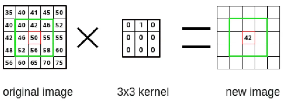
Convolution is a mathematical operation which is fundamental to many common image processing operators. Convolution provides a way of ”multiplying together” two arrays of numbers, generally of different sizes, but of the same dimensionality, to produce a third array of numbers of the same dimensionality [30].

In image processing, one of the input arrays is normally a grayscale image, while the second array is a smaller matrix known as convolution matrix, filter or kernel. In this context an operator that implements convolution produces an output image as simple linear combinations of the input pixel values.

A filter can be thought as a sliding window moving, from left to right and from top to bottom, across the original image. Generally the filter moves through all the positions where it fits entirely within the boundaries of the image. At each shift, the filter produces a single output pixel, whose value is calculated by summing all the products between

(34)

2. CNN for Object Recogntion 20 the filter elements and the corresponding pixels.

Figure 2.2: A single step of convolution performed on 9 × 9 image and a 3 × 3 kernel. Figure 2.2 shows the output produced from a 3 × 3 filter at the center of 9 × 9 image. The resulting image highlights the characteristics enhanced by the filter used. As a result, in computer vision, several filters are used for different purposes. The more popular are:

• Gaussian filters: normally used to remove noise by taking average between the current pixel and a specific number of neighbours.

• High-pass filters: normally used to improve image details. • Emboss filters: normally used to enhance brightness differences. • Sobel filters: normally used to highlight edges.

Until now, we have only discussed one to one convolutions that apply a filter to single image. We can identify other two kinds of convolution:

• One to many convolution: when there are n filters and only one input image. In this case, each filter is used to generate a new image.

• Many to many convolution: when there is n filters and more than one input image. Each connection in between input and output images is characterized with specific different filters.

(35)

2.2 Convolutional Neural Network: an overview

Convolutional Neural Networks (CNNs) are a category of Feedforward Neural Net-works. Likewise, CNNs are made up of neurons with learnable weights and biases. Again, backpropagation is the algorithm used for training the network.

Historically, CNNs have been used in the context of image classification, indeed the typical CNN input is a multi-channeled image. In the last decades, the neuroscience community has proved that one of the unique ability of the human visual system is called perceptual invariance and it emerges from the complex (and generally hierarchi-cal) organization of connections in the brain. This and other studies, have directly inspired the architecture of CNNs.

The CNN multi-layer architecture resembles the organization of information in the human visual system in order to achieve robustness against shifting, distortion and scal-ing of objects.

Deep neural networks composed by only fully connected layers involve a huge number of parameters which would most likely lead to overfitting or it can just be wasteful in terms computation. Therefore, CNNs use convolutional layers which rely on ideas like local receptive fields and shared weights. Normally convolutional layers execute many to many convolutions. Each neuron of the layer performs a convolution where its weights are the values of the filter. Convolution layers involve a smaller number of weights respect fully connected layers. For example, when processing an image, the input image might have thousands or millions of pixels, but we can detect small, meaningful features such as edges with kernels that occupy only tens or hundreds of pixels [31]. This means that we need to store fewer parameters, which both reduces the memory requirements of the model and improves its statistical efficiency.

In brief, CNNs differ from other ANN models in that they are composed of a particular set of layers, such as convolutional layers or downsampling layers, which are inserted in a specific sequence.

(36)

2. CNN for Object Recogntion 22

2.3 Layers used to build CNN

One of the key characteristics of CNN is the particular set of layers which composes the network. In literature, it is possible to identify three main kinds of layers which are described in the following sub-sections.

2.3.1 Convolutional layer

The first layer in a CNN is always a convolutional layer. In a convolutional layer only small localized regions of the input are connected to every hidden neuron. That region in the input image is called the local receptive field for the hidden neuron. Figure 2.3 shows a 5 × 5 local receptive field which corresponds a filter of the same size. The filter numeric values represent the weights of the hidden neuron. Likewise convolutions in computer vision, each filter convolves over all the locations of the input image, producing an output image called activation map.

Figure 2.3: A 5 × 5 filter convolving an input volume and producing an activation map [7].

It is worth noting that, the extent of the connectivity along the depth axis of the local receptive field is always equal to the depth of the input volume. For example, if the receptive field is 5 × 5 and the input image is [32 × 32 × 3], then each neuron will

(37)

have weights to a [5 × 5 × 3] region in the input volume.

Moreover, convolutional layers implement parameter sharing. Basically, parameter sharing constrains the neurons to use the same weights and bias. Thus, because the fil-ter is shared, all the neurons in the convolutional layer detect exactly the same feature, just at different locations in the input image. Informally, a feature is a type of input pattern (an edge in the image) that will cause the neuron to activate. For this reason, the activation map is also called feature map. The number of feature maps corresponds to the depth (third dimension) of the convolution output volume.

The importance of detecting different image features explains why a convolutional layer produces several feature maps. In fact, generally, a convolutional layer increase the dimensionality of the input volume on the depth axis (third dimension). A real world example is the Krizhevsky architecture [2] that won the ImageNet challenge in 2012. Figure 2.4 shows 90 of the 96 filters learned by Krizhevsky at the first convolutional layer. The size of each filters is [11 × 11 × 3], and each one is shared by the 55 ∗ 55 neurons in one feature map.

Figure 2.4: Example filters learned by Krizhevsky [2]. In general the output volume is controlled by three hyperparameters:

• Depth: this parameter sets the amount of filter used equivalent to the amount of feature map produced.

(38)

• Stride: this parameter controls how we slide the filter. For instance, when the stride is 1, the filter moves one pixel at time.

• Zero-padding: if greater than zero, this parameter pads the input volume around the border with a number of zeros according to the specified value.

The following formula can be used to find the size (first two dimensions) of the output volume:

(W − F + 2P )/S + 1

where W is the input volume size, F represents the filter size of the convolutional layer, S and P are the stride and the amount of zero padding respectively.

2.3.2 ReLU Layer

Generally, after each convolutional layer, it is convention to apply a ReLU (Rectified Linear Units) layer (or activation layer). The ReLU layer applies the rectifier activation function:

f (x) = max(0, x)

to all of the values in the input volume. Practically speaking, this layer just changes all the negative activations to 0. As mentioned in chapter 1, there are other activation functions like tanh and sigmoid. In the last decade, Researchers have found out that ReLU layers work far better [32] because the network is able to train a lot faster without making a significant difference to the accuracy. Additionally, it helps to alleviate the vanishing gradient problem.

2.3.3 Pooling layer

A Pooling layer applies a form of non-linear downsampling. The aim of downsampling is to reduce the spatial size of the representation. In this category maxpooling layer are the most popular. This pooling layer uses the MAX operation on a subregion of the input (filter), normally of size 2 × 2, with a stride of the same length. Hence, it outputs

(39)

Figure 2.5: Example of maxpooling with a 2 × 2 filter and stride 2 [6].

the maximum number in every subregion that the filter convolves around. For three-dimensional input, every depth slice is downsampled along both width and height.

In figure 2.5, the output of maxpooling layer with a 2 × 2 filter and stride 2 is shown. There are two main benefits from using pooling layers in CNN:

1. The number of parameters is drastically decreased, thus lessening the computation cost.

2. The threat of overfitting is reduced, thus the network’s ability of generalization is improved.

As an aside, some CNNs use 1x1 convolutions as a feature pooling technique. For example, an image of 150 × 150 with 30 features on convolution with 10 filters of 1 × 1 would result in size of 150 × 150 × 10. In this context, 1 × 1 convolution can be useful because we operate on 3-dimensional volume, although, on two dimensional input, it would be pointless.

2.3.4 Fully connected layer

In chapter 1, the fully connected layer it has been introduced as the typical layer of an ANN. In a CNN they are normally used for learning non-linear combinations of high level

(40)

features. Essentially, the aim of convolutional layers is to provide an invariant feature space, and the aim of fully-connected layer is learning a function (generally non-linear) in that space.

2.4 CNN architecture

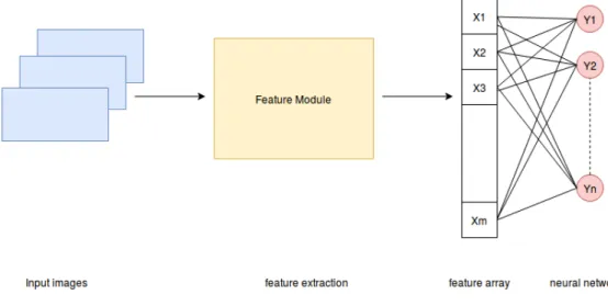
In this section we discuss how the layers, described in the previous section, are stacked together to form a CNN. The architecture of a CNN can be divided into three parts, as shown in figure 2.6. First of all, a CNN receives in input a sequence of digital images; then the input is given to a feature extraction module which generates an array of features; finally this array is delivered to a full connected neural network that produces the results.

Figure 2.6: General CNN architecture divided in its fundamental parts

The feature extraction module is composed by an alternation of three layer types: CONV(Convolutional), ReLU and POOL (Pooling). The most common architecture follows the pattern:

IN P U T → [[CON V → RELU ]] ∗ N → P OOL?] ∗ M

where * represents repetition and POOL? an optional Pooling layer. Usually 0 ≤ K ≤ 3 and 0 ≤ N ≤ 3.

(41)

Instead, the full connected neural network is composed by an alternation of FC (Fully connected ) and RELU layers. It can be described by the following pattern:

[F C → RELU ] ∗ K → F C where again 0 ≤ K ≤ 3.

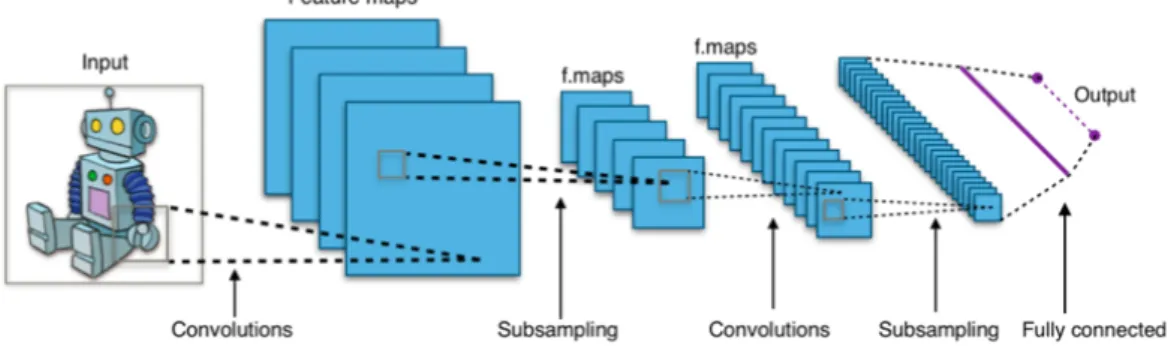
Figure 2.7 provides an overview of a typical CNN architecture with 5 layers. All the convolutions are many to many, i.e. each feature map has a neuron that can be connected with two or more feature maps of the previous layer.

Figure 2.7: A simple CNN architecture [8]

In this section we have discussed the typical CNN architecture, however there many variants depending on the task. For instance, there are CNN without final neural net-work. In this case other classifier, such as Support Vector Machine, can be used.

2.5 CNN training

The backpropagation algorithm, introduced in the previous chapter, computes (an-alytically using the chain rule) the gradient of a CNN loss function with respect to its weights. The backpropagation (BP) is used as a gradient computing technique by the gradient descent optimization algorithm. Gradient descent is currently the most common and established way of optimizing CNN loss functions. Training a CNN from scratch with the gradient descent algorithm is not the only strategy. Gradient descent and other CNN training strategies are described in the following subsections.

(42)

2.5.1 Gradient descent

The procedure of repeatedly evaluating the gradient of a loss function and then performing a parameter update is called gradient descent. This algorithm is widely used to train CNNs. A code implementation of gradient descent looks as follows:

1 f o r i in range( i t e r a t i o n s ) :

2 w e i g h t s g r a d = e v a l u a t e g r a d i e n t ( l o s s f u n , t r a i n d a t a , w e i g h t s ) 3 w e i g h t s += − s t e p s i z e ∗ w e i g h t s g r a d

This simple loop is at the core of all Neural Network libraries.

Besides, there are some variants of gradient descent, which differ in how much data we use to compute the gradient of the loss function:

• Batch gradient descent: it computes the gradient of the cost function with respect to its parameters for the entire training dataset. Thus, we need to calculate the gradients for the whole dataset to perform just one update. It can be very slow and expensive in terms of memory (dataset could not fit in RAM). BGD is guaranteed to converge to the global minimum for convex error surfaces and to a local minimum for non-convex surfaces.

• Stochastic gradient descent: it computes the gradient of the cost function with respect to its parameters for one training example at each step. Hence, SGD performs a parameter update for each training example with a high variance that cause the loss function to fluctuate heavily. SGD’s fluctuation allows it to jump to new and potentially better local minima. On the other hand, this ultimately complicates convergence to the exact minimum. SGD is usually much faster than BGD since it updates weights more frequently.

• Mini-batch gradient descent: a compromise between BGD and SGD, is to compute the gradient against more than one training example at each step. MGD performs an update for every mini-batch of n training examples. This approach reduces the variance of the parameter updates, which can lead to more stable convergence. Mini-batch gradient descent is typically the algorithm of choice when training ANN. Common mini-batch sizes range between 50 and 256, but can vary for different applications.

(43)

Even though SGD technically refers to using a single example at a time to evaluate the gradient, the term SGD is employed even when referring to mini-batch gradient descent, where it is usually assumed that mini-batches are used.

2.5.2 Training strategies

When training a CNN from scratch (with random initialization), it is relatively rare to have a dataset of sufficient size. Moreover, training from scratch might take a long time to complete (days, weeks).

Instead, it is common to pre-train a deep CNN (base network) on a very large dataset and then use its the weights as an initialization for a second CNN (target network). This scenario is known as Transfer Learning. There are two main strategies, in the context of transfer learning:

• Fine-tuning the ConvNet: it consists in copying the first n layers of the trained base network to the first n layers of the target network and in fine-tuning the copied weights of target network by continuing the backpropagation (training). The choice of whether or not to fine-tune the first n layers of the target network depends on the size of the target dataset and the number of parameters in the first n layers [33]. This strategy is motivated by the observation that earlier layers of a ConvNet learn more generic features (e.g. Gabor filters or color blobs) which should be useful to many tasks, instead later layers of the ConvNet are progressively more specific to the details of the classes contained in the original base dataset. When transferred layers are not fine-tuned, copied weights are left frozen, meaning that they don’t change during training on the new task.

• ConvNet as fixed feature extractor: as mentioned in section 2.4, the central module of a CNN works as feature extractor. In this strategy, again, layers from the trained base network are copied into the target network. Then, the last fully-connected layers are removed from the target network, which is treated as fixed feature extractor for a new dataset. For every image in the dataset, a corresponding feature vector is extracted and used to train a linear classifier (e.g. Linear SVM or Softmax classifier).

(44)

2.6 Visualizing and understanding deep CNN

In the last years there has been considerable improvements in the creation of high-performing architectures and learning algorithms for deep neural networks. On the other hand, the understanding of how these large neural models operate has lagged behind. In fact, it is tough to understand exactly how any trained neural network works due to the huge number of interacting, non-linear parts. This has led to consider neural netowrks as black boxes, especially deep neural networks composed by several layers.

According to [34] there are different approaches that try to understand, through features visualization, what is learned at each level of a DNN. One approach is to interpret the function computed by each individual neuron. Past studies in this vein divide into two different camps: dataset-centric and network-centric. Examples from the two classes will be discussed in the following subsections.

2.6.1 Dataset-centric approach

Dataset-centric techniques require both a trained DNN and running data through that network. One famous dataset-centric approach is the deconvolution method [9] which highlights the portions of a particular image that are responsible for the firing of each neural unit (within its feature map) at any layer in the model. This technique is based on a Deconvolutional Network (deconvnet). A deconvnet uses the same components of a convnet (convolutional, pool layers etc.) but in reverse (unpool, rectify, etc.), thus it maps features to pixel. At the beginning an input image is forwarded throughout the convnet, then to examine a given layer activation, one of the relative feature maps is passed as input to the attached deconvnet layer. The deconvnet layer reconstruct the activity in the layer beneath that gave rise to the chosen activation. This is then repeated until input pixel space is reached.

Figure 2.8 shows the top nine activations in a random subset of feature maps across the validation data, projected down to pixel space using the deconvolutional network approach in [9].

(45)

Figure 2.8: Visualization of features in a fully trained model [9]

2.6.2 Network-centric approach

Network-centric techniques require only the trained network itself. Consequently, they investigate directly a DNN without any data from a dataset. In this category, as an example, Simonyan et al. (2013) [10] use the gradient ascent technique, introduced by [35], in order to address the visualization of deep image classification CNNs.

The procedure is related to the CNN supervised training procedure, but in this case the optimization is performed with respect to the input image (weights are fixed to those found during the training stage). In basic terms, the objective of the optimization is to maximize the score (neuron response in the final layer) of a given class of images. In the first step (forward pass) of the algorithm, an image with random pixel colors is forwarded throughout the network. Also, it is selected the class score to be maximized. In the second step (backward pass), the gradient of the class score with respect to the input image is performed. The pixel color values are updated adding the product between the

(46)

gradient result and the learning rate. This two-step process is repeated until satisfying results are achieved.

Figure 2.9: Pictures produced by maximization of three different class scores [10] Figure 2.9 shows three images produced by maximizing a given class score: bell pep-per, lemon , husky. The three pictures resemble some recognizable features of the related class models. It was worth mentioning that these results were achieved by employing L2-regularization. In fact, without such a regularization form, would have been harder to recognize class appearance models.

The visualization of such images suggest qualitatively which invariant features the net-work has learned from different classes.

(47)

CORe50

“In God we trust; all others must bring data.”

- professor W. Edwards Deming In this chapter, CORe50 a new dataset and benchmark for continuous object recognition, is introduced. In the first section few datasets similar to CORe50 are briefly described. In section two, an overview of CORe50, with details on its design and aim, is provided. Finally, the process for integrating the depth information in CORe50 is illustrated.

3.1 Existing datasets and their limitations

In the context of object recognition, CORe50 is a dataset for incremental learning. Therefore, we present only existing datasets suitable for incremental learning strategies. Most of the datasets described in the following sub-sections have been used by Maltoni and Lomonaco [36] for accuracy evaluation of incremental learning strategies. In par-ticular, we focus on the limitations of such datasets in order to justify the creation of CORe50.

(48)

3. CORe50 34

3.1.1 iCubWorld28

iCubWorld28 is a significant dataset in the robotics field. It consists of 28 different objects organized into 7 categories. For each object are acquired 220 images (128 × 128 pixels in RGB format) for both train and test set. This acquisition collects one dataset of more than 12K images and runs over four days (4 dataset).

Maltoni and Lomonaco [36] reach an averaged accuracy of 75% using the fine-tuning strategy over the CaffeNet network. In the context of Incremental Learning, the main limitations of this dataset are:

• the small number of sessions: 4; • the small number of objects: 28; • the maximum resolution of 128 × 128;

• the limited background variation: only indoor acquisition

3.1.2 Big Brother

The BigBrother dataset is composed by 23.842 70 × 70 gray-scale images of faces belonging to 19 competitors of famous Italian reality show. The dataset is divided into training set, test set and an additional set of images, called ”updating set “. The updating set is provided for incremental learning/tuning purposes.

Again, according to [36], fine-tuning the CaffeNet with a pretrained model is the most effective strategy, even though the best reached averaged accuracy is smaller (of some points) respect the ICubWorld28. The BigBrother dataset has a small number of images compared to the iCubWorld28 dataset. Moreover, it presents only faces and it is not useful for generic object recognition.

3.1.3 NORB dataset

NORB is one of the best dataset to study invariant object recognition. It is composed by 50 uniform-colored objects under 36 azimuths, 9 elevations, and 6 lighting conditions (for a total of 194,400 individual images). The objects are 10 instances of 5 classes. The

(49)

image resolution and image format are 640 × 480 and RGB respectively. Furthermore, temporally coherent video sequences can be generated from NORB by randomly walking the 3D variation space.

Thus, the NORB dataset contains a significant number of frames and variations. On the other hand, the images recorded are untextured toys without natural background.

3.2 CORe50: an overview

Maltoni and Lomonaco introduce CORe50 [3] as a new dataset and benchmark for continuous object recognition. Being specifically designed for incremental learning strate-gies, Core50 is well-suited to this purpose. As we have seen in the previous sections, several datasets used for incremental learning lack of fundamental properties.

CORe50 consists of 50 domestic objects belonging to 10 classes: markers, plug adapters, balls, mobile phones, scissors, light bulbs, cans, glasses, cups and remote con-trols (see Figure 3.1)

Figure 3.1: The 50 different objects of CORe50. Each column denotes one of the 10 categories [3].

CORe50 supports classification at object level (50 classes) or at category level (10 classes). The former (the default one) is much more challenging because objects of the same class are very difficult to be distinguished under certain poses. The dataset has

(50)

3. CORe50 36

been collected in 11 distinct sessions (8 indoor and 3 outdoor) characterized by differ-ent backgrounds and lighting (see Figure 3.1). For each session and for each object, a 15 seconds video (at 20 fps) has been recorded with a Kinect 2.0 sensor delivering 300 RGB-D frames. The presence of temporal coherent sessions (i.e., videos where objects gently move in front of the camera) is another key characteristic since temporal smooth-ness can be employed to ease object detection, improve classification accuracy and to address semi-supervised (or unsupervised) scenarios. The camera point of view coincides with the operator eyes. Objects are hand hold by the operator, therefore relevant object occlusions are often produced by the hand itself. Moreover, a point-of-view with objects at grab-distance is appropriate for a number of robotic applications.

Figure 3.2 depicts one frame of the same object throughout the eleven session. Note the variability in terms of illumination, background, blurring, occlusion, pose and scale.

Figure 3.2: One frame of the same object throughout the 11 acquisition sessions [3].

3.2.1 RGB-D dataset

An important feature of CORe50 is the opportunity to run experiment exploiting the depth information of the images. The Kinect RGB-D cameras provide dense depth estimations together with color images at a high frame rate. During acquisition, the Kinect records 1024 × 575 RGB + 512 × 424 Depth frames. A central region, in the acquisition interface, points out where the object should be kept (see Figure 3.3). This can be used for reducing (cropping) the RGB frame size to 350 × 350.

(51)

Figure 3.3: The Acquisition interface [3].

has been exploited temporal information to crop from each 350 × 350 frame a 128 × 128 box around the object. In most cases, the motion-based tracker implemented to this purpose fully contains the objects in the crop window. Nevertheless, sometimes objects can extend beyond border due to tracking imperfections.

Moreover, since the motion based tracker is not always able to identify an object in the first frames of a session, less images have been acquired for the cropped dataset.

In summary, three dataset have been produced:

• CORe50 350x350 rgb: composed by 165,000 350 × 350 images: 11 sessions × 50 objects × 300 frames per session.

• CORe50 128x128 rgb: composed by 164,866 128 × 128 images: 11 sessions × 50 objects × ∼ 300 frames per session.

• CORe50 512x424 depth: composed by 164,740 512 × 424 images: 11 sessions × 50 objects × ∼ 300 frames per session.

Note that also CORe50 512x424 depth presents less images. This is due to the fact that, during acquisition, the Kinect depth sensor was not perfectly synchronized with

RGB-D Object Recognition for Deep Robotic Learning