Cancer classification using gene expression data with deep learning

(1)

Cancer Classification using Gene

Expression Data with Deep Learning

Güray Gölcük

Supervisor: Prof. Stefano Ceri

Advisor: Dr. Arif Çanako˘glu

Department of Electronics, Informatics and Bioengineering

Polytechnic University of Milan

This dissertation is submitted for the degree of

Master of Science

(2)

(3)

Abstract

Technological advances in DNA sequencing technologies allow sequencing the human genome for a low cost and with in a reasonable time span. This advance conduces to a huge increase in available genomic data, enabling the establishment of large-scale sequencing data projects. Producing genomic datasets, which describe genomic information in particular, we concentrate on our attention on gene expression datasets which describe healthy and tumoral cells for various cancer types. The purpose of this thesis is to apply deep learning to classification of tumors based on gene expression.

Two different Deep Learning approaches for analyzing the genomic data. First one is to create a feed-forward network (FFN) with supervised learning, second one is using ladder network with semi-supervised learning [42] . Main purpose of both approaches is to perform binary classification, cancerous or healthy as the outcome, over the Cancer Genome Atlas (TCGA) database.Two cancer types selected from TCGA. Breast cancer is selected because it has the highest available amount of sample in all cancer types in TCGA. The reason for kidney cancer to be selected is because, it has the one of the highest mortality rate among rest. Moreover, three feature extraction method, PCA, ANOVA and random forests, employed to preprocess the selected datasets. Experiments show that, FFN reaches the acceptable accuracy rate but fails to reach a stabilization. On the other hand, ladder network, outperforms the FFN in both accuracy and stabilization meaning. Effects of feature extraction method shows us that, main goal as accuracy is reached by PCA & ladder network combination, main goal as performance is reached by ANOVA & ladder network combination.

(4)

(5)

Abstract

Le innovazioni riguardanti le tecniche di sequenziamento del DNA stanno permettendo analisi del genoma umano sempre più veloci ed economiche. Ciò ha provocato un aumento considerevole dei volumi di dati disponibili riguardanti il genoma umano, permettendo l’instaurazione di progetti di sequenziamento su larga scala. In questo contesto di database genomici, ci concentreremo sui dati di espressione genica, i quali descrivono cellule tumorali e sane provenienti da diversi tipi di tessuto. Lo scopo di questa tesi è di applicare il deep-learning alla classificazione dei tumori in base all’espressione genica.

Ci siamo concentrati su due approcci fondamentali per l’analisi dei dati genomici. Il primo consiste nella creazione di una rete Feed-Forward (FFN) per l’apprendimento supervi-sionato, il secondo utilizza una Ladder Network tramite apprendimento semi-supervisionato. L’obiettivo principale di entrambi gli approcci è di eseguire classificazione binaria, avente tumore o sano come risultato. Come dataset abbiamo utilizzato The Cancer genome Atlas (TCGA) e in particolare ci siamo concentrati su due tipi specifici di tumore: tumore della mammella e ai reni. Questa scelta è principalmente dettata dalla più alta disponibilità di sam-ples per questi due tipi di tumore. Abbiamo utilizzato tre differenti tipi di feature extraction, PCA, ANOVA and random forest.

Gli esperimenti hanno mostrato che FFN raggiunge un accuratezza accettabile ma fallisce in quanto a stabilità dei risultati. D’altra parte la Ladder Network sorpassa FFN sia in accuratezza che in stabilità. Gli effetti della feature extraction mostrano che la migliore combinazione per quanto riguarda l’accuratezza è PCA con Ladder Network, mentre per quanto riguarda le performance la combinazione ANOVA e Ladder network prevale.

(6)

(7)

List of figures

1.1 The cost of genome sequencing over the last 16 years [27] . . . 2

1.2 The amount of sequenced genomes over the years [17] . . . 3

2.1 An excerpt of region data . . . 8

2.2 An excerpt of metadata . . . 8

2.3 Example of map using one sample as reference and three samples as experi-ment, using the Count aggregate function. . . 12

2.4 The web graphical user interface of GMQL . . . 14

2.5 High-level representation of the GMQL system . . . 15

3.1 TCGA Cancer Datasets with corresponding sample numbers . . . 18

4.1 Example of linear regression estimation . . . 26

4.2 Decision Surface . . . 28

4.3 Steps of random forest algoritm [22] . . . 30

4.6 Perception . . . 33

4.7 Activation functions: sigmoid, tanh, ReLU . . . 34

4.8 MLP (FFN) with one hidden layer . . . 35

5.1 Final structure . . . 41

5.2 Best accuracy with kidney data . . . 42

5.3 Best accuracy with breast data . . . 43

5.4 Effects of number of features . . . 44

6.1 Example of semi-supervised input data . . . 46

6.2 Steps of classification based on smoothness assumption . . . 47

6.3 Structure of 2 layered ladder network . . . 49

(12)

6.5 Structure of model that is used for classification of TCGA data . . . 51 6.6 Accuracy in kidney data when PCA is used for feature selection method . . 53 6.7 Accuracy in breast data when PCA is used for feature selection method . . 53 6.8 Accuracy in kidney data when ANOVA is used for feature selection method 54 6.9 Accuracy in breast data when ANOVA is used for feature selection method 54 6.10 Accuracy in kidney data when Random Forest is used for feature selection

method . . . 55 6.11 Accuracy in breast data when Random Forest is used for feature selection

(13)

List of tables

A.1 Error rate for TCGA kidney data with 200 features with 1 hidden layer . . . 65

A.4 Error rate for TCGA kidney data 700 features with 1 hidden layer . . . 66

A.5 Error rate for TCGA kidney data with random forests with 1 hidden layer . 66 A.6 Error rate for TCGA breast data with 200 features with 3 hidden layer . . . 66

A.7 Error rate for TCGA breast data with 300 features with 3 hidden layer . . . 67

A.8 Error rate for TCGA breast data with 500 features with 3 hidden layer . . . 67

A.9 Error rate for TCGA breast data 700 features with 3 hidden layer . . . 67

A.10 Error rate for TCGA breast data 1000 features with 3 hidden layer . . . 67

A.11 Error rate for TCGA breast data with random forests with 3 hidden layer . . 68

B.1 Error rate for TCGA kidney data with 200 features with ladder . . . 69

B.5 Error rate for TCGA kidney data with random forests with 1 hidden layer . 70 B.6 Error rate for TCGA breast data with 200 features with ladder . . . 70

B.7 Error rate for TCGA breast data with 300 features with ladder . . . 71

(14)

(15)

Chapter 1 Introduction

1.1 DNA Sequencing

The DNA sequencing is a process of detecting the exact sequence of the nucleotides (adenine, guanine, cytosine, and thymine ) that creates the DNA. The advancements in the DNA sequencing technologies greatly effects the discoveries the in biological and medical science [24, 32]. Developments in DNA sequencing also helps biotechnology and forensic studies significantly [18].

Sequencing a whole DNA has been very complex and an expensive task. Breaking DNA into smaller sequences and reassembling it into a single line is still complex, even so, improvements into computer science and discoveries of new methods over past two decades, makes it cheaper and faster.

(16)

Fig. 1.1 The cost of genome sequencing over the last 16 years [27]

It is evident from the Figure 1.1 that in 2001, DNA sequencing per genome cost 100M dollar however after 2015, the cost has been significantly drop down to the order of 1K dollar. Improvements in DNA sequencing technology keep up with Moore’s law. 1 till 2007. After the introducing of Next Generation Sequencing (NGS) technologies, sequencing cost fall sharply and reach the value of 1K dollar today [44].

1_{According to Moore’s law the number of transistors in dense integrated circuits meaning the performance}

(17)

1.2 Analysis of Genomic Data 3

1.2 Analysis of Genomic Data

Fig. 1.2 The amount of sequenced genomes over the years [17]

The drop in the sequencing cost allows a huge increase in sequenced genome data as shown in the Figure 1.2. Increase in sequenced genomic data made it possible to establish huge genomic projects such as Human Genome Project [9], The Encyclopedia Of DNA Elements (ENCODE) [11] and the 1000 Genomes Project Consortium [10]. These projects ceaselessly gather and store sequencing data. Importance of big data analyzing techniques shines after this point. Big data analysis are essential to utilize collected data efficiently.

Sequence Data analysis can be broadly separated into three categories [37].

• Primary Analysis (Base Calling): Converts raw data into nucleotides with respect to the changes in electric current and light intensity.

• Secondary Analysis (Alignment & Variant calling) Maps the short sequence of nucleotides into reference sequence to determine variation from.

• Tertiary Analysis: (Interpretation) Analyses variant to estimate their origin, impact, and uniqueness.

(18)

Out of these three categories, the tertiary analysis is the most important one, since knowledge gathering from sequenced data handled in the tertiary analysis.

GenData 2020 project, which introduced in 2013, was concentrate on tertiary analysis of genomic sequence data. GenoMetric Query Language (GMQL) and Genomic Data Model (GDM) is the most important outcomes of this project. GMQL is query language that works with heterogeneous datasets such as sequenced genomic data while GDM is the general data model for mapping genomic features with its metadata. GMQL also have interface for Python an R which are most commonly used in data analysis. More information on GMQL can be found on Chapter 2.

1.3 Machine Learning with Genomic Data

Machine learning is a data analysis method that allows the automation of model building and learning with given input data. It is a subset of artificial intelligence based on the idea that machines should learn through experience. With machine learning, computers could use pattern recognition to find hidden insights without any explicit programming. In comparison to the traditional biological computational methods, machine learning has been put into practice with the research on the binary or multiple cancer classification with genomic data [49, 53], For instance, Stacked Denoising Autoencoder (SDAE) [13] , Fuzzy Support Vector Machine (FSVM) [33] and Deep Belief Networks (BDN) [3] have been proposed to do binary and multi-class classification to genomic data.

Deep learning is a branch of machine learning with more complicated algorithms which can model features with high-level abstraction from data. It has achieved the state-of-the-art performance in several fields such as image classification [29, 46, 50], semantic segmentation [31] and speech recognition [25]. Recently, deep learning methods have also achieved success in computational biology [47, 4]. This thesis is the continuation of similar work of Tuncel [52], classification of cancer types with machine learning algorithms, through the deep networks. The goal of this thesis is to analysis the effects of the feature selection methods on the final accuracy of the created Deep Neural Networks. The study can be divided into two part. First part is the creation of the feed forward network and effects of the feature selection algorithm on final accuracy and second part is implementation of the ladder network structure for binary classification, and effects of feature selection algorithms. The input data is the breast and cancer data from the Cancer Genome Atlas (TCGA) database.

This thesis is arranged as follows: In Chapter 2 background for GMQL method is presented. In Chapter 3 information on the input data is presented. Chapter 4 theoretical background for data analyzing is explained, it includes machine learning, neural networks

(19)

1.3 Machine Learning with Genomic Data 5 and used methods for feature extracting. Chapter 5 describes the created feed forward network and the results achieved. Chapter 6 introduces the ladder network, and explains implementation for binary classification. Chapter 7 compares the final result of the both network and effects of the feature extraction on them. Finally, conclusions and possible future work are discussed in Chapter 8.

(20)

(21)

Chapter 2 Summary of Data Extraction Method

2.1 Genomic Data Model (GDM)

GDM acts as a general schema for genomic repositories. The GDM datasets are a collection of samples. Each sample has two parts, region data, and metadata. Metadata describes the sample-specific properties while region data describes the portions of the DNA. [7]. Each GDM dataset has a corresponding data schema that has few fixed attributes to represent the coordinate of the regions and identifier of the samples. The fixes attribute which represents the region information consists of a chromosome, the region that chromosome belongs to, left and right ends of the chromosome and the denoting value of the DNA strand that contains the region. There may be other attributes besides fixed ones that have information on DNA region. Metadata stores information about the sample with format-free attribute-value tuples. Figure 2.1 illustrates an excerpt of GDM region data. As seen, First five columns are the fixed attributes of the region data that represents the region information. The last column, on the other hand, is the p-value of the region significance in this case. Figure 2.2 illustrates sample-specific metadata properties. The first column of both figures (id) maps the region data and metadata together.

(22)

Fig. 2.1 An excerpt of region data

(23)

2.2 GenoMetric Query Language (GMQL) 9

2.2 GenoMetric Query Language (GMQL)

GMQL is high-level query language which is designed to deal with large-scale genomic data management. The name genometric, come from its ability to deal with genomic distances. GMQL is capable to deal with queries with has over thousands of heterogeneous dataset and it is suitable for efficient big data processing [52].

GMQL combines the traditional algebraic operation with domain-specific operations of bioinformatics, which are spastically designed for genomics. Therefore it supports the knowledge discovery between millions of biological or clinical samples, which satisfies the biological conditions and their relationship to experimental [34].

The inclusion of metadata along with processed data in the many publicly available experimental datasets, such as TCGA, makes the initial ability of GMQL to manipulate the metadata is exceptionally important. GMQL operation forms a closed algebra meaning result are denoted as new dataset derived from operand. Hence, region-based operations build new regions, metadata based operations traces the root of each sample outcome. GMQL query, expressed as a sequence of GMQL operations, follows the structure below.

<variable> = operation(<parameters>) <variables>

Each variable indicates GDM dataset. The operator can apply one or more operand to construct one result variable. Each operator has its own parameters. Most of the GMQL op-erations are relational opop-erations, which are mostly algebraic opop-erations which are modified to fit the need of genomics data.

2.2.1 Relational GMQL Operations

• SELECT operator applies on metadata and selects the input samples that satisfy the specified metadata predicates. The region data and the metadata of the resulting samples are kept unaltered.

• ORDER operator orders samples, regions or both of them; the order is ascending as default and can be turned to descending by an explicit indication. Sorted samples or regions have a new attribute order, added to the metadata, regions or both of them; the value ofORDER reflects the result of the sorting.

• PROJECT operator applies on regions and keeps the input region attributes expressed in the result as parameters. It can also be used to build new region attributes as scalar expressions of region attributes (e g., thelength of a region as the difference between itsright and left ends). Metadata are kept unchanged.

(24)

• EXTEND operator generates new metadata attributes as a result of aggregate functions applied to the region attributes. The supported aggregate functions areCOUNT (with no argument),BAG (applicable to attributes of any type) and SUM, AVG, MIN, MAX, MEDIAN, STD (applicable to attributes of numeric types).

• GROUP operator is used for grouping both regions and metadata according to distinct values of the grouping attributes. For what concerns metadata, each distinct value of the grouping attributes is associated with an output sample, with a new identifier explicitly created for that sample; samples having missing values for any of the grouping attributes are discarded. The metadata of output samples, each corresponding a to given group, are constructed as the union of metadata of all the samples contributing to that group; consequently, metadata include the attributes storing the grouping values, that are common to each sample in the group.

• MERGE operator merges all the samples of a dataset into a single sample, having all the input regions as regions and the union of the sets of input attribute-value pairs of the dataset samples as metadata.

• UNION operator applies to two datasets and builds their union, so that each sample of each operand contributes exactly to one sample of the result; if datasets have different schemas, the result schema is the union of the two sets of attributes of the operand schemas, and in each resulting sample the values of the attributes missing in the original operand of the sample are set to null. Metadata of each sample are kept unchanged. • DIFFERENCE operator applies to two datasets and preserves the regions of the first

dataset which do not intersect with any region of the second dataset; only the metadata of the first dataset are maintained.

2.2.2 Domain-specific GMQL Operations

Domain-specific operations are created specifically to respond the genomic management requirement needs.

• COVER operation is widely used in order to select regions which are present in a given number of samples; this processing is typically used in the presence of overlapping regions, or of replicate samples belonging to the same experiment. The grouping option allows grouping samples with similar experimental conditions and produces a single sample for each group. For what concerns variants:

(25)

2.2 GenoMetric Query Language (GMQL) 11 – FLAT returns the union of all the regions which contribute to the COVER (more precisely, it returns the contiguous region that starts from the first end and stops at the last end of the regions which would contribute to each region of theCOVER). – SUMMIT returns only those portions of the result regions of the COVER where the maximum number of regions intersect (more precisely, it returns regions that start from a position where the number of intersecting regions is not increasing afterwards and stops at a position where either the number of intersecting regions decreases, or it violates the max accumulation index).

– HISTOGRAM returns the nonoverlapping regions contributing to the cover, each with its accumulation index value, which is assigned to the AccIndex region attribute.

• JOIN operation applies to two datasets, respectively called anchor (the first one) and experiment (the second one), and acts in two phases (each of them can be missing). In the first phase, pairs of samples which satisfy the joinby predicate (also called meta-join predicate) are identified; in the second phase, regions that satisfy the genometric predicate are selected. The meta-join predicate allows selecting sample pairs with appropriate biological conditions (e.g., regarding the same cell line or antibody). • MAP is a binary operation over two samples, respectively called reference and

ex-periment. The operation is performed by first merging the samples in the reference operand, yielding to a single set of reference regions, and then by computing the aggregates over the values of the experiment regions that intersect with each reference region for each sample in the experiment operand. In other words, the experiment regions are mapped to the reference regions.

The output ofMAP operation is called genometric space, which is structured as a matrix. In this matrix, each column indicates the experiment sample and each row indicates the reference of the region while matrix entries are scalar. Resulting matrix can be easily inspected with heat maps, which can cluster the columns and/or rows to display the patterns, or processed and analyzed by any other matrix-based analytical process. To summarize MAP operation allows the quantitive readings of stored experiments with respect to reference region. If the reference region of the biological data is not known, Map function allows extracting the most interesting reference region out of the candidates.

Fig. 2.3 illustrate the effect of MAP operation on a small portion of the genome; Input has one reference sample with 3 regions and three corresponding mutation experiment

(26)

Fig. 2.3 Example of map using one sample as reference and three samples as experiment, using the Count aggregate function.

samples, Output has three samples, which locates int he same region as the reference sample, as well. The features of reference sample correspond to the number mutations that are interacting with those regions. The final result can be explicated as a (3x3) genome space.

2.2.3 Utility Operations

• MATERIALIZE operation saves the content of a dataset into the file system, and registers the saved dataset in the system to make it seamlessly usable in other GMQL queries. All datasets defined in a GMQL query are, temporary by default; to see and preserve the content of any dataset generated during a GMQL query, the dataset must be materialized. Any dataset can be materialized, however, the operation is time expensive. Therefore to achieve the best performance it is suggested to materialize the relevant data only [7].

2.2.4 Biological Example

The biological example below uses the MAP operation from domain-specific GMQL op-erations to count the regions that are peaked in each ENCODE ChIP-seq sample that is intersected with a gene promoter. After that, for each sample, it projects over the promoters

(27)

2.2 GenoMetric Query Language (GMQL) 13 with eat least one intersecting peak and counts these promoters. As the last step, it extracts the top three samples with highest count number of such promoters

HM_TF = SELECT(dataType == 'ChipSeq') ENCODE; PROM = SELECT(annotation == 'promoter') ANN; PROM1 = MAP(peak_count AS COUNT) PROM HM_TF; PROM2 = PROJECT(peak_count >= 1) PROM1;

PROM3 = AGGREGATE(prom_count AS COUNT) PROM2; RES = ORDER(DESC prom_count; TOP 3) PROM3;

Further details about GMQL basic operators, GMQL syntax and relevant examples of single statements and a notable combination of them are available at GMQL manual1and GMQL user tutorial2.

2.2.5 Web Interface

In order to make GMQL publicly available and user-friendly for the ones with limited computer science experiment, a web interface designed and implemented by GeCo group. Two services developed for this purpose. REST API and web interface. Both of them have the functionalities to search the genomic features dataset and biological/clinical metadata, which are collected in system repository from ENCODE and TCGA, and build GMQL queries upon them. GMQL interface can efficiently run such queries with thousands of samples with few heterogonous dataset. Moreover, with user management system, private datasets can also be upload to the system repository and used in the same way with the available datasets in the system. GMQL REST API planned to used them with the external systems such as GALAXY [20], which is another data integration system and workflow that is commonly used in bioinformatics, or other systems that can run REST services over HTTP.3. Figure 2.4 illustrates the web user interface of GMQL.

1_{GMQL Manual:}_{http://www.bioinformatics.deib.polimi.it/genomic_computing/GMQL/doc/}

GMQL_V2_manual.pdf

2_{GMQL User Tutorial:}_{http://www.bioinformatics.deib.polimi.it/genomic_computing/GMQL/}

doc/GMQLUserTutorial.pdf

(28)

Fig. 2.4 The web graphical user interface of GMQL

2.2.6 Python Interface

Python interface of GMQL, PyGMQL, is an alternative to the web interface of the system. Python library interact with the GMQL through Scala back-end. With PyGMQL it is also possible for users to write GMQL queries with the same syntax as standard Python pattern. PyGMQL can be used locally or remotely. GMQL queries executed on the local computer when it is used locally while it is executed on the remote GMQL server when it is used remotely. It is also possible to switch between remote and local mode during the pipeline analyzing stage. Moreover, PyGMQL introduces efficient data structure to analyze GDM data and provides specifically developed data analysis and machine learning packages to manipulate genomic data. Figure 2.5 describe the interaction between the user and GMQL with PyGMQL in a high-level representation.

(29)

2.2 GenoMetric Query Language (GMQL) 15

(30)

(31)

Chapter 3 Tertiary Analysis of the RNA-Seq Data

Numerous studies made in past years to examine the transcriptome 1 to identify healthy or diseased. Study of Golub et al. [21], about distinguishing the types of severe leukemia cancer is one of the pioneering work in this area. After that, many ensuing studies on both supervised and unsupervised on expression data is done. Preceding studies on transcriptome analysis (DNA microarrays) were only available for few types of cancer yet they still did not have enough sample most likely fewer than a hundred. DNA-Seq technology of today gives more precise and complete quantification of the transcriptome with the publicly available dataset. For instance, TCGA dataset contains 33 different types of cancer, including 10 rare cancers and hundreds of samples [19, 39, 2]. Figure 3.1 shows the available cancer types and the amount of samples in TCGA dataset. The interested readers may refer to [54, 40, 23, 45, 38] for a detailed explanation of the RNA-Seq technology.

1_{Transcriptome is the sum of all RNA molecules in a cell or a group of cells that are expressed from the}

(32)

Fig. 3.1 TCGA Cancer Datasets with corresponding sample numbers

3.1 Characteristics of RNA-Seq Data

3.1.1 High Dimensionality

Gene expression data has a considerably small amount of sample while a relatively high amount of features (genes). However, this characteristic is very common an expected in RNA-Seq and DNA Microarray technologies. As it can be clearly seen in Figure 3.1, only few cancer type has more than 500 sample. Despite that, each sample has approximately 20k genes. These phenomena is called the curse of dimensionality. Curse of dimensionality has 2 important traits that make data hard to deal.

1. o have a large number of features which may be irrelevant in a certain comparison of similarity, have corrupt the signal-noise ratio.

2. In higher dimension, all samples "seem similar"

There few feature extraction methods to overcome the high dimensionality problem. Chapter 4 introduces few methods that are used in this thesis.

3.1.2 Biases of the RNA-Seq Data

Having biases is yet another characteristic of RNA-sequential data. Some of the biases need to be taken care before deeply analyzing the data. First bias occurs because of the

(33)

3.1 Characteristics of RNA-Seq Data 19 technical issues regarding the sequencing depth [51]. Observations in RNA-seq data suffer from a strong dependency on sequencing depth for their differential expression calls, and each observation might have a different number of total reads. Thus, values on the dataset do not only depend on the expression value of the genes but also depends on the depth of sequence matrix. The difference in the length of genes in the RNA-seq data causes another, more critical bias. Longer the genes more the readings it gets. This tendency cause several problems for analysing methods such as classification and clustering [40]. Hence, these need to be solved before analyzing in detailed, otherwise, the final results can not be trusted. Normalization techniques need to be performed in order to clear up the problems with biases. Normalization also helps to improve the convergence speed of various machine learning algorithms. Normalization also necessary for feature reduction techniques such as PCA (explained in Section4.1.5), to allow all genes to have an opportunity to contribute the analysis. PyGMQL implements two methods for data normalization. One for shifting the mean value of every feature (gene) to zero. Another for reducing the variance of every feature to the unit variance. By applying those normalization techniques, we can assure that all of the genes are equally weighted for the classification or clustering.

3.1.3 Missing Values

RNA-Seq data commonly contain missing values like most of the experimental datasets. Classification approaches are not robust in presence of the missing values. Therefore missing value problem should be solved. The most simple solution to deal with the missing problem is to erase the samples to minimize the effects of incomplete datasets. However, considering the amount of sample in TCGAS datasets, erasing might not be a "smart" approach. De Souto et al. [14] pointed that it is common for the gene expression datasets to have up to 5% of missing values, which could affect up to 90% of the genes. Another method is filling the missing values with 0. Yet this approach performs poorly in terms of estimation accuracy. More advanced approach is instead of filling with 0, missing values filled by mean or median values of its corresponding column so the effects of the missing values over the general set minimized in computations. Filling missing values, with random values from the original dataset is another approach to solve this problem.

3.1.4 Unbalanced Distribution

Even though the cost of DNA sequencing falls around 1K$, the amount is not small enough for collecting the sequential data casually.Also, finding volunteers that allows sharing their DNA information on public domains is hard to find. As a result, most of the samples in

(34)

the available data collections are cancer positive. Unbalancing in the samples make the data unfavorable for direct feed to Deep Learning network. Methods explained in bleow is necessery to sole this problem

3.1.5 Dealing with Imbalanced Data

Imbalanced input data most of the time cause the predictions of DNN model to give prediction highly on one label. There are few methods to prevent them.

Up-sampling / Down-Sampling

Up-samplingand Down-sampling basically means to increase or decrease the sample of desired class. Up-sampling means, randomly duplicating the samples of the class, which has smaller sample amount until the balanced ratio between the classes is reached while Down-samplingmeans, instead of taking the whole samples from the overly populated class, just takes the same amount of sample with the other class so the final dataset will be balanced. Since the amount of sample in the data is already too small, down-sampling of the cancerous data is not logical. Furthermore, up-sampling of healthy data does not just fail to stabilize the result, but also fails the train data. Training accuracy moves around 50% as same as null hypothesis.

There is also another method named SMOTE [8] published for up-sampling, which introduced a new way to create new samples. SMOTE calculate the k nearest neighbors for each minority class observations. Depending upon the amount of oversampling needed, it creates a synthetic example along the line connecting the observation with k random nearest neighbors. However this method might be risky. There is a possibility for newly created synthetic data to indicate complete new life form, and there is not any way to check it. Because of the this reason, SMOTE is passed.

Penalized weight

Penalized the weight, of the class with superior sample number, in the logistic regression function or in the loss calculation step have possibility to solve the imbalanced data problem. Proportioned Batch

Imbalanced data may not be a problem if the input batch that is used to feed training step has the same proportion of classes with the whole training data.

(35)

3.2 Loading TCGA Data into Repository 21

3.2 Loading TCGA Data into Repository

The original TCGA data consist of 31 different types of cancer. There are 9.825 samples with 20.271 diverse genes. Only two cancer types (kidney and breast) selected for classification test in deep learning. Breast data selected number of samples , which is the highest amount included in TCGA dataset, and kidney is selected randomly from the rest. In the raw data, samples do not have values for all the genes sequences so these missing values are filled with the mean of that gene expression values to not change the outcome. Also, data normalization is performed in order to remove the biases described in section 3.1.2. How to load and preprocess the data is explained in code snippet 3.1. Whole code can be seen in Github repository [1]. 1 i m p o r t gmql a s g l 2 p a t h = ’ . / D a t a s e t s / t c g a _ d a t a / f i l e s / ’ 3 # t h e n o r m a l i z e d c o u n t v a l u e i s s e l e c t e d 4 s e l e c t e d _ v a l u e s = [’ n o r m a l i z e d _ c o u n t ’] 5 # we a r e o n l y i n t e r e s t e d i n t h e g e n e s y m b o l 6 s e l e c t e d _ r e g i o n _ d a t a = [’ g e n e _ s y m b o l ’] 7 # a l l m e t a d a t a a r e s e l e c t e d 8 s e l e c t e d _ m e t a _ d a t a = [ ] 9 g s = g l . ml . G e n o m e t r i c S p a c e ( ) 10 # t o l o a d t h e d a t a 11 g s . l o a d ( p a t h , s e l e c t e d _ r e g i o n _ d a t a , s e l e c t e d _ m e t a _ d a t a , 12 s e l e c t e d _ v a l u e s , f u l l _ l o a d = F a l s e ) 13 # m a t r i x r e p r e s e n t a t i o n 14 g s . t o _ m a t r i x ( s e l e c t e d _ v a l u e s , s e l e c t e d _ r e g i o n _ d a t a , d e f a u l t _ v a l u e =None ) 15 # c o m p a c t r e p r e s e n t a t i o n o f r e g i o n and m e t a d a t a 16 g s . s e t _ m e t a ( [’ b i o s p e c i m e n _ s a m p l e _ _ s a m p l e _ t y p e _ i d ’, 17 ’ m a n u a l l y _ c u r a t e d _ _ t u m o r _ t a g ’,’ b i o s p e c i m e n _ s a m p l e _ _ s a m p l e _ t y p e ’] ) 18 19 f r o m gmql . ml . a l g o r i t h m s . p r e p r o c e s s i n g i m p o r t P r e p r o c e s s i n g 20 # p r u n i n g t h e g e n e s t h a t c o n t a i n more t h a n %40 m i s s i n g v a l u e s 21 g s . d a t a = P r e p r o c e s s i n g . p r u n e _ b y _ m i s s i n g _ p e r c e n t ( g s . d a t a , 0 . 4 ) 22 # m i s s i n g v a l u e i m p u t a t i o n 23 g s . d a t a = P r e p r o c e s s i n g . i m p u t e _ u s i n g _ s t a t i s t i c s ( g s . d a t a , method =’ min ’) 24 # g e n e s t a n d a r d i z a t i o n 25 g s . d a t a = P r e p r o c e s s i n g . t o _ u n i t _ v a r i a n c e ( g s . d a t a )

(36)

(37)

Chapter 4 Theoretical Background

This chapter provides basic knowledge for machine learning, neural network and deep learning concepts, that are used during thesis.

4.1 Machine Learning

Machine learning is one of the many areas in artificial intelligence that gives computers to ability to learn without being specifically programmed. The main idea behind the machine learning is, regardless of the instructions to solve a problem, constructing a model with an acceptable amount of data, which can produce valuable predictions of the solutions. In consequence, machines learning is about various models, which use various methods to learn by adapt and improve their result from experience. "A computer program is said to learn from experience E with respect to some class of tasks T and performance measure P if its performance at tasks in T , as measured by P , improves with experience E " Mitchell [36]. Machine learning can be applied in many fields, such as financial services, health-care, customer segmentation , transportation and so on. In this thesis, it is used a binary classification task with TCGA data. Main goal is to create a model which can minimize the differences between predictions ˆyi= ( ˆy1, ˆy2, ..., ˆyn) and desired labels yi= (y1, y2, ..., yn) of

input xi= (x1, x2, ..., xm). The i corresponds to instance of the predictions while m and n

corresponds to the total number of input and output instances, respectively.

There are three subfields of machine learning; supervised learning, unsupervised learning and semi-supervised learning.

(38)

4.1.1 Supervised Learning

Supervised learningis where the input variables and the output variables are already de-termined and a learning algorithm is used to learn how to map the input to the output. In other words, the supervised learning algorithms learn by inspecting the given inputs x and desired outputs y with correcting the predictionsyi. There are several supervised learning

algorithms such as Linear Regression (LR), K-nearest Neighbors (KNN), support vector machine, decision trees, Naïve Bayes classifier in the literature.

4.1.2 Unsupervised Learning

Unsupervised learningis where the input data do not contain any information of correspond-ing output variables. The main goal of unsupervised learncorrespond-ing is to find meancorrespond-ingful patterns in distribution or model the underlying structure to increase the understanding of the input data. It is called unsupervised because unlike the supervised learning there is no "correct answer" or supervisor to control the learning process. Algorithms are free to make their own connections and discover new structures in order to interpret the data. Most common use of unsupervised learning is cluster analysis.

4.1.3 Semi-supervised Learning

Semi-supervised learningis placed between supervised and unsupervised learning, it involves the function estimation on labeled and unlabeled data. The main goal of semi-supervised learning is to use unsupervised learning to make predictions for unlabeled data and feed these data into supervised learning to predict the new data. Most of the real world machine learning problems are in the semi-supervised category since collecting labeled data could be expensive, time-consuming while collecting unlabeled data is relatively easier cheaper and easier to collect.

Semi-supervised learning, as an idea is the most similar learning method for the human and animal brain. “We expect unsupervised learning to become far more important in the longer term. Human and animal learning is largely unsupervised: we discover the structure of the world by observing it, not by being told the name of every object.” LeCun et al. [30]

Regression and classification are the two essential problems of the supervised learning. Regression is used to model the correlation between input samples and targets which are continuous while the targets of classification are categorical. To make it clear with example, classification is classifying the given genomic data as "cancerous" or "healthy", which is the

(39)

4.1 Machine Learning 25 classification task handled in this thesis, while regression example could be estimating the market price of the certain house.

4.1.4 Linear Regression

Linear Regression is an statistical method that enables to figure out the statistical rela-tionships between two numerical variables. Supposed that the input data is in form of (x1, y1), ..., (xn, yn), where the x is the input value and y is the corresponding output while xi

and yiare real numbers with i within 1,...,n and n refers to the sample size, the model that

predict the numerical response f (X ) = Y by assuming there exist a linear relation between the input and the output. The relation between input and output can be mapped as Equation (4.1).

Y = β0X+ β1 (4.1)

In Equation (4.1), β0 and β1 are the unknown constants that represent the slope and

intercept of the predicted regression line. Main goal is, by training the model, finding a best fitting line through all data.

(40)

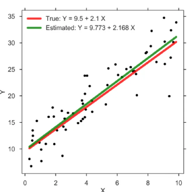
Fig. 4.1 Example of linear regression estimation

An example with one variable linear regression is shown in Figure 4.11. Figure consistent of multiple black points with two straight lines. The green line consist of the predicted values

ˆ

yifor each possible value of xiwhile the red line indicates the correct outputs yi. The distance

between each black point and and green line is called prediction error or loss.

The better estimations is done by minimizing the loss function. The loss functionL is the sum of all individual losses over the instances of X. Assuming ei= yi− ˆyirepresent the

1_{Source of the picture is}

(41)

4.1 Machine Learning 27 ithindividual loss, the loss function becomes:

L =

_∑

n

i=1

ei (4.2)

The aim is to find the β0and β1values, which can minimize theL . Thus the important

thing is to choice of selection the best loss function for the problem. The most commonly used one is residual sum of squares (RSS):

RSS= n

∑

i=1 e2_i (4.3)

4.1.5 Classification

Classification used for predicting the numerical responses. The main goal is to create a model, which can assign the given input vector into available classes accurately based on the training set and labels. In most of the cases, the input classes are disjoint meaning each sample could only belong to one and only one class. Therefore, input space separates into decision regions which is called decision boundary or decision surface [6].

(42)

Fig. 4.2 Decision Surface

Figure 4.22illustrates the decision surface. It consists of 2 different points, 0 and X that indicates the class labels and 2 lines that draws a boundary between points such as when the new data comes If it not visualized in very controversial spot, the class it belongs to will be easy to predict.

Classification task consist of four main phases, preprocessing, feature extraction, training and lastly classification.

Preprocessing: In preprocessing stage, raw data, which is gathered from source, handled before employed as an input. This phase is necessary since most of the cases, input data obtained is noisy, incomplete or /and inconsistent. Preprocessing involves data-related tasks such as cleaning, transformation, reduction and so on. Preprocessing steps that is used to prepare the input data for the task handled in this thesis is explained in Section 3.1 to deal with problems of the raw data.

Feature Extraction: Next phase is feature extraction. Features are the domain-specific measurements, which have relative information to create the best possible representation of

(43)

4.1 Machine Learning 29 the input. For classification, most relevant features need to be extracted from raw data. There is a lot of feature selection methods in literature such as ANOVA, PCA, LDA and etc. all with their own advantages and disadvantages.

As a task in this thesis is a classification problem with input data having a lot of features, three feature extraction algorithms, all chosen from commonly used as feature extracting methods from related genomic classification papers; ANOVA, PCA, Random Forest are introduced in this part.

• ANOVA (Analysis of Variance) : ANOVA is the one of the mostly used feature section methods that is used in machine learning to deal with high dimensionality problem. Proposed by Bharathi and Natarajan [5], it uses F-test to select the features that maximize the explained variance.

• Random Forests: Random forests is another commonly used feature selection algorithm [16]. Random forests is set of decision tree classifiers. Each node splits dataset into two, based on the condition value (impurity) of every single feature. This way similar instance to falls in the same set. For classification purposes, Gini impurity or information gain/entropy is chosen to be impurity condition. This structure calculates the effect (how much it decrease the impurity) of every feature on the tree. The flowchart for random forests can be seen in the Figure 4.3. 7

• PCA Principal Component Analysis : Rather than feature selection, Principal Com-ponent Analysis is a dimensionality reduction technique that used to transform high-dimensional dataset into a smaller dimension. Reducing the high-dimensionality of dataset also reduces the size of space, number of freedom of hypothesis. Algorithms work faster when they need to deal with a smaller dimension and visualization become simpler.

PCA transforms the dataset to a lower dimension one with a new coordinate system. In that coordinate system first axis indicates the first principal component which has the greatest variance in data. With PCA it is possible to explain 95-97% of the variance in the input dataset with fewer PCA compare to the original dataset. For instance, 500 PC is enough to explain 98% of the variance in the TCGA kidney dataset, while it only explains 89% of the variance in breast dataset. Since PCA focus to find the principal component with the highest variance, the dataset should be normalized, so that each attribute has an opportunity to contribute the analysis.

Training: In this phase as also explained before, model trains to give the most accurate prediction as possible.

(44)

Fig. 4.3 Steps of random forest algoritm [22]

Classification: In classification, the created model assign input into one of the available classes based on created the decision rules.

Classification problem consists of three main parts. First, the frequency of the classes to occur in the input data, probability distribution. Second, characteristic features to define the relationship between input and output for separating the classes. Third, defined loss function which penalized the inaccurate predictions such that the final cost should be minimized as it mentioned in Subsection 4.1.4 (Regression) [35]. Therefore most of the classification tasks in real world, based on the probability theory. Probabilistic model outputs a vector which contains the probability of all possible classes, to show the degree of certainty.

After training model is finalized and the training is done, model can be used to predict the possible class of the new data. After training model is finalized and the training is done, the model can be used to predict the possible class of the unseen data. However, every classifier that is built tries to memorize the training set. Training constantly may cause the model to memorize the training set which will end up with poor performance when dealing with new

(45)

4.1 Machine Learning 31 data while getting perfect accuracy with the training set. These phenomena called over-fitting. What is needed is, to create a model which is capable of generalizing so that it performs well new data as well as the training data. Over-fitting also could occur because of the complexity of the model.It is hard for a model to generalize the inputs with complex structures. There are few methods to detect the over-fitting, one of which is explained in Section 5.3.

Figure 4.43shows three models which are trained with three different complexity level on top. The figure on the bottom shows the training and prediction error rate. Training error rate getting lower and lower which the increase in complexity, however, prediction error rate starts to increase after some point. Top right graphic, shows the over-fitting example which has the perfect curve to include all existing data yet it gets poor performance when to deal with a new sample. On the other hand, the graph in the middle has pattern instead of following each data point which has worse training error but better prediction error. In order

(46)

to create a "good" model which is capable of dealing with new data, the complexity of the model and the amount of training steps should be chosen carefully.

4.2 Deep Neural Network

The deep network is a subsection of machine learning, that models the data using multiple layered artificial neurons. The idea is copying the interactions of the actual nervous system. The figure illustrates the real neural network, as seen, dendrites bring input signals where axons pass the information from one cell to another cell through synapses.

Artificial network "learns" by adopting changes in the synaptic weights of the network. The architecture has parallelly distributed structure with an ability to learn, which make it possible to solve complex classification tasks with in reasonable time.

.

4.2.1 Perception

Perception is a feed forward network that builds the boundaries of a linear decision, which is a fundamental part of the neural networks. Figure 4.64,illustrates the perception in the ANNs. Input signal can be represented as weights. Transfer function sums the response and feed the resulting signal to the activation function. Based on the activation function’s threshold, output is determined. To simplify it can be represent as wighted sum of inputs:

(47)

4.2 Deep Neural Network 33 y= n

∑

j=1 w_jx_j+ w₀ (4.4) where: n= The number of outputs

w₀= Value of interception from bias unit x0= +1

Fig. 4.6 Perception

For linear cases, binary threshold can be used as an activation function (e.g. step function) to determine the output. Then, output of the system decided as a:

o(x) = sgn(w · x) (4.5) where: sgn(y) =    +1 if y > 0 −1 otherwise (4.6) On the other hand, to represent non-linear functions, non-linear activation functions are necessary. There are few non-linear activation functions in the literature. Figure 4.7 illustrates tanh, sigmoid and rectified linear unit (ReLU), which also three of the most common ones.

(48)

Sigmoid function compress the input in to [0; 1] range, where 0 means it is not activated and 1 means it has maximum frequency. Tanh, compress it in to [-1 ; 1] range with same logic. Relu has an output of 0 if the input is smaller than 0, output the the raw input otherwise

Fig. 4.7 Activation functions: sigmoid, tanh, ReLU

sigmoid(x) = 1 1 + e−x (4.7) tanh(x) =e 2x_{− 1} e2x_{+ 1} (4.8) ReLU(x) = max(x, 0) (4.9) Tanh can be considered as a scaled version of sigmoid function:

tanh(x) = 2sigmoid(2x) − 1 (4.10) There are a lot of approaches for perception to predict the correct class label by finding the optimum weight vector of the training data. The most common one known as the perception learning rule. If the classification problem is linearly separable, perception learning rule always converges the optimum weights in finite time [43]. For this approach, all weights are initialized with random values between (-1, +1 ). Then perception applies to each training example. With each wrong classification, weights are updated by adapting them at each iteration with equation (4.11) until the output is correctly classified.

(49)

4.2 Deep Neural Network 35 where:

∆wi= α(t − o)xi

4.2.2 Multilayer Perception

Single perception is limited to linear mapping, so it fails to solve complex tasks. To solve complex tasks, more comprehensive model, which is capable of performing the arbitrary mapping. With perception, it is possible to build larger and more practical structure that can be described as a network of perceptions named multilayer perception (MLP). The basic structure of MLP could also be called as feedforward network (FFN) since it has a direct connection between all layers. General MLP has three main layers; one layer for input, one or more layer as a hidden layer and one layer for the output. Hidden layer is "hidden" from inputs and outputs as it is indicated in the name. Learning task of the complex model by extracting features from input data, handled in the hidden layer. MLP with one hidden layer structure is known as two-layer perception, is shown in Figure 4.8.

Fig. 4.8 MLP (FFN) with one hidden layer

Furthermore, as proved in [12] and [26], an MLP with a single hidden layer represents a universal function approximation. A two-layer perception can be written mathematically as: y= f (x) = ϕ(b(2)+W(2)(ϕ(b(1)+W(1)x))) (4.12)

(50)

where:

W(1),W(2)= Weights b(1), b(2)= Biases

ϕ = activation function

In the equation (4.12), ϕ(b(1)+W(1)x)) forms the hidden layer and the rest establish the output layer.

4.2.3 Training an DNN

Deep neural network learns by minimizing the loss function by changing the parameters (θ = {W(∗), b(∗)}) of the model in training. stochastic gradient descent (SGD) is the one of the most common approach to used for learning the parameters. The gradients of a loss function are calculated by using the back-propagation (BP ) algorithm, then the results fed to the SGD method to update the weights and biases.

Stochastic Gradient Descent

SGD algorithm updates the set of parameters θ incrementally after each epoch. An epoch indicates the number of times all of the training input used to update the parameters. All training samples get through the leaning phase in one epoch before parameters are updated. SGD calculates the approximation of the true error gradient error based on a single training sample, instead of compute the gradient of the error based on the all training sample like in gradient descent (GD). Thus DNN can train faster with SGD, since calculating the approximation is faster. wj:= w + ∆wj (4.13) ∆wj= α n

∑

i=1

(target(i)− out put(i))x(i)_j (4.14) where:

α = Learning rate After each epoch, weights in Equation (4.13), updated as:

(51)

4.2 Deep Neural Network 37 Backpropogation

To use SGD in multi-layer networks, gradient of the loss function is needed to be computed. Backpropogation is the most common method used to overcome this problem. In backpro-pogation, calculating the partial derivatives ∂ L/∂w of the loss function L with respect to

some weight w is enough to analyse the cahnge in the loss with the change of weights. Using mean squared error (MSE) as cost function one output neuron over all n examples is:

L= 1 2 n

∑

j=1 (tj− yj)2 (4.16) where: t= target label

y= output of the perceptron

Lis scaled by 1₂ for mathematical convenience of Equation (4.22). Error gradient is calculated in equation (4.17) to use SGD

∆wk j= −α

∂ L ∂ wk j

(4.17) where a node in layer k is connected to a node in layer j. The result is taking negative We take the negative because the change of the weights are in the direction of where error is decreasing. because weight changes are in the direction where the error is decreasing. Using chain rule gets us:

∂ L ∂ wk j = ∂ L ∂ yj ∂ yj ∂ xj ∂ xj ∂ wk j (4.18) In Equation (4.18), xj is the weighted sum of the inputs being passed to jth node and

yj= f (xj) is the output of the activation function. As a result:

∂ xj

∂ wk j

= y_k (4.19)

If the sigmoid function is used as an activation function, the derivative becomes: d f(x)

(52)

Plugging it in to Equation (4.18):

∂ yj

∂ xj

= yj(1 − yj) (4.21)

Finally, the first partial derivative of the remaining part ∂ L

∂ yj, which is the derivative of

Equation (4.16):

∂ L ∂ yj

= −(tj− yj) (4.22)

Putting the whole thing together, algorithm for the output-layer case become: Overall, putting all things together, we form the algorithm for the output-layer case:

∂ L ∂ wk j

= −(tj− yj)yj(1 − yj)yk (4.23)

Chain rule for the propagation of the error, : ∂ L ∂ wk j = ∂ L ∂ yj ∂ yj ∂ xj ∂ xj ∂ wk j (4.24) First two partial derivatives in equation (4.24), can be donated as δi and the rest is the

derivate of the weighted sum of the inputs wji:

∂ L ∂ yj

= −

_∑

δiwji (4.25)

As a result, it can be written as equation (4.26) for the hidden layers: ∂ L

∂ wk j

= −

_∑

(δiwji)yi(1 − yj)yk (4.26)

(53)

Chapter 5 FFN Methodology

In this chapter, the details of the implementation steps for the first part of the thesis, creating a Feed-forward network for binary classification of TCGA data is described. This chapter introduces the result of our first attempts to solve the classification problem. Throughout this chapter, the following steps will be covered respectively: data preprocessing, feature extraction and FNN architecture.

5.1 Preprocessing

As briefly mentioned in the Section 4.1.5 preprocessing is an important step to properly analyze the input data. The problems of input data are explained in 3.1. To summarise, input data have three problems to solve in preprocessing phase. It has a bias on expression values, missing values in samples and input data is unbalanced. Normalization function of PyGMQL library is used to normalize the input data to overcome the bias problem of the raw input. Missing values filled with its mean value of the respective column. Sequence of the input data is change to guarantee each batch has the same proportion of the input as whole data.

5.2 Feature Extraction

The most important thing in feature extraction is to select most relevant features, whose has enough information about input to differentiate the different classes easily. Optimal solution is the selecting most important features by hand. However for this case, it is not possible to managed that. So as a feature extracting, PCA with 200, 300, 500, 700 principal components, ANOVA with 200, 300, 500, 700 selected features and random forest with importance level higher than .001, .0005, .0001 selected for experiment to find the optimum

(54)

model and the optimum feature selection method. The threshold of PCA algorithm is 606 principal components for kidney data. With 606 principal components, the 99.999% of the variance in the input data is covered. It is not possible to include more principal components. Therefore 606 the highest amount to feature selected for kidney database to make comparison simple.

5.3 Train, Test, Validation split

Deep learning needs two inputs. Once for training the data, one for testing the trained model. It is important to use different samples for training and test to actually trigger learning process. Sealing the test information from training cause the model to learn from training data without knowing the answer.

Since input data will be used for classification(in our case), the proportion of the labels in the splits must be preserved. Stratified split algorithms are perfect for this job. Python library sklearn have a method named stratified shuffle split[sklearn] that can handle this part. It takes random partitions the data into k independent subsets of the same size.Then it trains the model using k-1 subsets and tests it on the last subset. This procedure is repeated k times assuring that each subset is used once as the test data. The k results are later averaged to produce the final result while preserving the label proportions. Input Data split into 2 parts, 80% training dataset, 20% test dataset as the most suggested train-test ratio.

However, every system tends to memories the outcomes. After continues training with the same train- test data allow the system to have an idea about the content of test data indirectly. To prevent that another dataset completely separated from train and test is needed. After training done, instead of checking the accuracy of test data (which can be over-fitting because of indirect learning ) the accuracy of separate validation dataset gives the correct result. Thus, training data needed to split again. Splitting training dataset into two with 75% , 25% proportion for validation dataset give us the final parts of parts 60% for training dataset, 20% validation datasetand 20% test dataset.

Data predation steps explained above (Section 5.1, 5.2, 5.3) are essential for any classifi-cation tasks. The resulting output is used for the input feed for both FFN, explained in this chapter, and ladder network explained in Chapter 6.

5.4 FFN Structure

FFN follows the steps mentioned in the Section 4.2. Input TCGA data is fetch from the GMQL server with the GMQL web interface and loaded into the local repository, explained

(55)

5.5 Results & Discussion 41 in Section 3.2. For FFN, expression values of the selected genes are used for the input training feed. Corresponding input training labels, gathered from the TCGA metadata as healthy or cancerous.

Various combinations of different complexity level is tried to prevent over-fitting which is mentioned in Subsection 4.1.5. Best results are gathered by using FFN consist of three layers, one for input, one for hidden and one for output. Nodes in the input layer changes evenly depending on the feature selection method and how many features are extracted. Hidden layer consist of 20 nodes and output layer has nodes same number as output class, which is two in this case. ReLU used for activation function. The used batch size is 60, trained with 60 - to 80 epochs. For training stochastic gradient descent optimization is used and cross-entropyused for the calculation of the loss function. Figure 5.1 illustrates the final structure of used FFN model. I1...Inindicated the input nodes where the n is the number of

the extracted features. H1...Hmindicates the hidden nodes where m is 20 for this case and

O1...O2indicates the output nodes: one for healthy, one for cancerous.

..

.

..

.

I₁ I2 I₃ I_n H₁ Hm O1 O2 Input layer Hidden layer Ouput layer

Fig. 5.1 Final structure

5.5 Results & Discussion

Highest achieved validation accuracy can be seen in Figure 5.2 and Figure 5.3. Best results, the lowest error rate, achieved with PCA (300 principal components) as feature extraction method, and 2 layer neural network structure (5.1) as model structure for TCGA kidney

(56)

data. PCA (700 principal components) for feature extraction and 4 layered neural network as structure achieves best result, the lowest error rate, for TCGA breast data.

(57)

5.5 Results & Discussion 43

Fig. 5.3 Best accuracy with breast data

The feature extraction methods is absolutely necessary for this level of analysis. Deep learning do not have enough samples to find possible connections between all features. With out any feature selection method, input with all 20206 features, fails to improve the null hypothesis. The amount of features also affecting the learning accuracy, with too much feature involved, the model fails to predict new samples accurately. Figure 5.4 shows the general behavior through the effect of features over models prediction. The number of the features for the classification task is highly dependent on the input data. In other words, around 700 features are necessary for the model to have a good approximation on prediction new samples, in TCGA breast data, while only 300 features are enough with TCGA kidney data.

Taking into consideration that, 300 principal components of PCA can protect 94% of the variance in the kidney dataset, on the other hand it can only protect 82% of breast dataset. Therefore, in order to reach 94% of the variance, 400 additional principal components are required. As it is expected, the number of the features that preserve the accuracy are different for each dataset. The detailed result for each feature selection and method are available in the Appendix A.

(58)

Fig. 5.4 Effects of number of features

The discrepancy in datasets also affects the constructional complexity. 1-layered feed-forward network with small amount of hidden nodes is enough to train kidney data but it is too simple to train breast data. While overfitting/underfitting occurs with more complex structures when training kidney data, it is necessary to reach a decent model with breast data.

To summaries, both input datasets are trained to do binary classification task. Because of the discrepancy in dataset, different structures are necessary to obtain satisfactory results. PCA gives the best performance as a feature extraction method, followed closely by ANOVA. Random forest, on the other hand, has the worst performance, training barely improves the null hypothesis

Final accuracy can be considerable as exceptionally high, especially with kidney data (99%). However, model gives highly unstable results. As it can bee seen on the tables in Appendix A, system generally fails to improve the null hypothesis. Mostly, the model under-fits the healthy samples from input, which most probably occurs because of the imbalance in input data. However, stability of the model does not improve with any of the methods mentioned in 3.1.5. All in all, the created feed-forward model is not trustworthy for binary classification of TCGA data.

(59)

Chapter 6 Ladder Network with Semi-Supervised

learning

The created feed-forward network in Chapter 5 is failed to give a satisfying result. Even though the final accuracy is good, the stability of the system is not acceptable. The final opinion we can infer with is that the resulting model actually is not a trustful model. What is required to achieve a more stable structure that can reach an acceptable accuracy level result with a low amount of input data. Ladder network is satisfying these conditions. It achieves dropping the error rate to 1.06% with only 100 labeled examples with publicly known MNIST (Modified National Institute of Standards and Technology database) [15] dataset.

This chapter will consist of 3 sections: Section 6.1 explains the process of semi-supervised learning. Section 6.2 explains what is ladder network. Section 6.3 shows the ladder structure and illustrates the final accuracy results.

6.1 How Semi-Supervised Learning works

Semi-supervised learning uses supervised learning tasks and techniques to make use of unlabeled data for training. Generally, the amount of labeled data is very small, while the unlabeled data is much larger.

Figure 6.1 illustrates a visualization of semi-supervised input data. Grey point are the unlabled datas, where the black one and white one indicates different labels of unlabeled data.

(60)

Fig. 6.1 Example of semi-supervised input data

It is really hard to make sense when having very small number of labeled and unlabeled data, but when all unlabeled ones are seen 6.1, it can be worked out to process.

(61)

6.1 How Semi-Supervised Learning works 47

Fig. 6.2 Steps of classification based on smoothness assumption

Assuming, there is a structure underlying the distribution of data and labels are homo-geneous in densely populated space i.e. With smoothness assumption1, classification of the unlabeled data became much more easier to deal. Figure 6.2 shows steps of classification of unlabeled data based on smoothness assumption.

It has been found that the utilization of unlabeled data together with a small amount of labeled data can enhance accuracy extensively. In the most of the real world situation, collecting labeled data is very expensive while there is a lot of unlabeled data is on hand. Semi-supervised learning is best to be used in these kind of situations. Also, such learning system is very similar to how our brain works. For instance humans don’t need to see all versions of chairs to understand if the new object is a chair or not. Seeing a small number of chair sample (labeled data) with all past experiences (unlabeled data) help us to categorize the objects. Hence, semi-supervised learning is a rational model for the human brain.

Cancer classification using gene expression data with deep learning