Universit`
a degli studi di Roma
“Tor Vergata”
Radiative properties of complex
magnetic elements in the solar
photosphere.
Thesis Author:
Dr. Serena Criscuoli
Thesis Advisors:
Prof. Mark Rast, Prof. Francesco Berrilli
Thesis Coordinator:
Prof. Roberto Buonanno
The University of Rome “Tor Vergata”
in partial fulfillment of the requirements for the degree
of
Doctor of Philosophy in Astronomy.
mea verba dicata sunt.
these words are dedicated
1 Introduction: The Solar Magnetic Field 1
1.1 The Sun . . . 1
1.2 The Solar Magnetic Field . . . 2
1.3 Photospheric magnetic features . . . 6
1.3.1 Active regions: formation and evolution . . . 9
1.4 Solar Variability and Irradiance Variations . . . 10
1.5 Aim of the thesis . . . 13
2 Fractal dimension estimation of facular regions 14 2.1 Fractals: introduction . . . 14
2.2 Fractal dimension estimation of solar magnetic features . . . 17
2.3 Observations, processing and definitions . . . 20
2.3.1 PSPT data . . . 20
2.3.2 Data quality . . . 21
2.3.3 Feature identification . . . 21
2.3.4 Perimeter and area evaluation . . . 22
2.4 Fractal Dimension Estimator: The Perimeter Area relation . . . 23
2.5 Results . . . 25
2.5.1 Fractal dimension and feature size . . . 25
2.5.2 Temporal variation . . . 26
2.6 Comparison to previous results . . . 27
2.6.1 Fractal dimension and structure size . . . 27
2.6.2 Temporal variation . . . 27
2.7 Discussion of fractal dimension estimation . . . 28
2.7.1 Perimeter definition and pixelization effects . . . 28
2.7.2 Resolution and seeing effects . . . 30
2.8 Results interpretation . . . 32
3 A study of faculae photometric properties 34 3.1 On the importance of magnetic features contrast measurements . 34 3.2 Observations and data reduction . . . 36
3.2.1 PSPT data . . . 36
3.2.2 Magnetic regions identification technique . . . 36
3.3 Results . . . 38
3.3.1 Center to Limb variation . . . 38
3.3.2 Black body approximation . . . 40
3.3.3 Size and Activity Cycle dependence . . . 41
3.3.4 Observational limitations . . . 44
4 The flux tube model 49
4.1 The concept of Flux Tube . . . 49
4.1.1 Temperature stratification and photometrical properties . 52 4.2 The Magneto Hydro Dynamic Equations . . . 55
4.2.1 Magneto Hydrostatic Static Equations . . . 56
4.2.2 Formation and Destruction of Intense Magnetic Flux Tubes 58 4.2.3 Brief review of Numerical Codes of Magnetic Flux Tubes 59 5 The Radiative Transfer Equation and the Short Characteristic technique 63 5.1 The Radiative Transfer Equation . . . 63
5.1.1 The exact solution . . . 65
5.1.2 Moments of Intensity . . . 66
5.1.3 TE and LTE . . . 67
5.1.4 Radiation Matter interaction . . . 67
5.1.5 Rosseland Mean opacity . . . 68
5.1.6 Approximate solutions to the RTE . . . 69
5.2 Radiative Equilibrium Gray atmosphere . . . 72
5.3 Numerical solution to the RTE: The Short Characteristic . . . . 73
5.3.1 Propagating the intensity on the grid . . . 77
5.4 Quadrature techniques . . . 78
5.4.1 Carlson schemes . . . 79
5.4.2 Gauss Legendre scheme . . . 85
6 Preliminary Tests 86 6.1 Integration techniques . . . 86
6.2 Interpolation effects: Search Beam technique . . . 88
6.2.1 Conclusions . . . 95
6.3 Combined effects of integration and interpolation . . . 96
6.4 Eddington Barbier Atmosphere . . . 97
6.5 Quadrature techniques . . . 99
6.5.1 Conclusions . . . 103
7 A Flux Tube Model 105 7.1 NON magneto NON dynamic Flux Tube Models . . . 105
7.2 Tubes in NON radiative equilibrium . . . 107
7.2.1 Radiative Diffusion atmospheres with convection . . . 107
7.3 Atmospheres in radiative equilibrium . . . 110
7.3.1 Initial and boundary condition: Radiative Diffusion at-mospheres without convection . . . 110
7.4 Computational and Numerical Details . . . 113
8 Results 114 8.1 Physical properties of simulated magnetic flux tubes . . . 114
8.1.1 Models with Convection: Models C . . . 114
8.1.2 Radiative Equilibrium models . . . 117
8.2 Intensity profiles at constant optical depth . . . 125
8.3 Ratio of contrasts . . . 131
8.4 Comparison with Observations and Conclusions . . . 133
9 Conclusions and Future Work 135 A Appendix to Chapter 2 148 A.1 Fractal dimension measurement of Non-fractal objects . . . 148
A.2 von Koch snowflake . . . 149
A.3 Fractal dimension measurement of Fractional Brownian motion patterns . . . 151
B Appendix to Chapter 6 154 C Appendix to Chapter 7 156 C.1 Mixing Length models . . . 156
C.1.1 Generalization of Mixing Length Formulation . . . 158
C.1.2 Not radiating parcel . . . 158
C.2 Radiative Diffusion models . . . 159
D Appendix to Chapter 8 162 D.1 About the iso-optical depth surfaces and the intensity profile . . 162
D.2 Ratio of contrasts in quiet atmosphere . . . 164
1.1 The interior and the atmosphere of the Sun are ideally sepa-rated into layers. In the core energy is produced by nuclear reactions. The Radiative and the Convective zones are named after the predominant energy mechanism transport in these lay-ers. The photosphere is the lowest layer of the atmosphere that can be observed. Above it the chromosphere and the corona host several phenomena of magnetic origin (in the picture: flares and prominences). The flare, sunspots and photosphere, chromo-sphere, and the prominence are all clipped from actual images of
the Sun taken by instruments onboard on SOHO spacecraft. . . 3
1.2 Temperature as a function of height in the Solar atmosphere.
The layers at which lines and bands have stronger emissivity are also shown. Observations at different wavelengths thus allow to investigate different portions of the atmosphere. From Vernazza
et al. (1981). . . 4
1.3 Solar dynamo sketch. (a) At the minimum of activity the
mag-netic field is bipolar. (b) Because of the differential rotation a stronger and stronger toroidal component is created as the time passes. (c) Magnetic ropes eventually emerge forming loops whose foot points, because of the Coriolis force, are twisted.(d) and (e) More magnetic field emerges and spread. These loops form bipolar regions, with the polarities oriented as shown in (f). The migration toward the equator and the poles finally causes flux cancellation and reversal of the polarity of the field. The red sphere represents the radiative region and the blue net is the base of the photosphere. These two regions are separated by a convective unstable layer. Adapted from Dikpati and Gillman
(2006). . . 5
1.4 Classification of Solar Magnetic Features observed in the
Photo-sphere. From Zwaan (1987). . . 6
ages show that both faculae and sunspots are made up of smaller substructures. Faculae are in particular made up of smaller bril-liant elements. Full disk image: CaII K image from Rome-PSPT archive (2 arcsec/pixel). Inset on the left: 436.4 continuum, from Swedish Solar Telescope (0.04 arcsec/pixel). Inset on the right: CA II H, from Swedish Solar Telescope. The two high resolution images were acquired by G. Scharmer and K. Langhans. The SST is operated on the island of La Palma by the Institute for
Solar Physics of the Royal Swedish Academy of Sciences. . . 8
1.6 Solar calcium K line in quiet and plage regions. Adapted from
Skumanich et al. (1984). . . 9
1.7 a): TSI over the period 1950-1998. b): Spectral Irradiance. c):
Spectral Irradiance changes between 1989 (solar maximum) and 1996 (solar minimum). d): Fractional Irradiance change for the period as in panel c). At shorter wavelengths of the spectrum, Irradiance relative variations are higher (up to two orders) respect
to longer wavelengths. From Hansen et al. (2002). . . 11
2.1 Fractals are classified according to their self-similarity properties.
Here examples from the three categories described in the text are
shown. . . 16
2.2 When measured with smaller and smaller size rulers, the length
of coast of Britain increases. Scatter plots in log scale of coast length and ruler precision, are fitted by a straight line whose slope is ≈ −0.26. The fractal dimension is thus D ≈ 1.26. . . 17
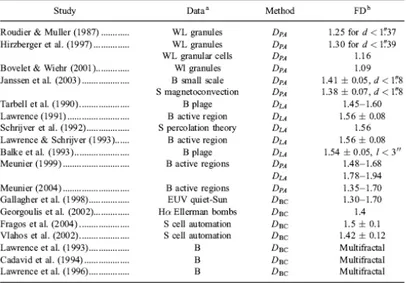
2.3 Summary of papers concerning fractal analyses of solar
mag-netic features. Studies have been carried out on different kind of data and with different estimators (PA:Perimeter-Area; BC: Box Counting; LA: minimum external box size-Area), so that fractal dimension estimates (right column) are often discrepant.
From McAteer et al. (2005). . . 18
2.4 Perimeter (in units of pixel) and Area (in units of pixels square)
in logarithmic scale of detected structures on OAR PSPT data taken during summer 2002. Continuous line is the fit to the whole set of data (D = 1.354 ± 0.005). Points at area greater than about 1000 pixels square are better approximated by a higher slope line. Horizontal line is the area window width over which
d1 is estimated. . . 23
2.5 Fractal dimension d1 versus area of bright features identified on
calcium images (∼ 2arcsec/pixel). Full circles: summers 2000-2005 OAR-PSPT. Open triangles: summer 2000-2005 MLSO-PSPT. Full triangles: summer 2005 OAR-PSPT. d1 increases fast with
object size at area smaller than 2000 Mm2. For larger areas, a
plateau is observed for summer 2005 OAR and MLOA data, and
a slow rise on the 2000-2005 OAR dataset. . . 24
the left represents the largest error bar, obtained for the largest
areas for year 2004. At area smaller than about 1000 Mm2 all
the curves overlap, while differences (not clearly correlated with
solar cycle) are observed at the largest areas. . . 25
2.7 Temporal variation of the fractal dimension D versus area for
selected OAR-PSPT calcium images and for different area range. Error bars in the case of fits performed on the whole dataset (circles) or at smallest objects (triangles) are smaller then the symbol size. Results obtained for the largest area are in good
agreement with results obtained by d1 estimator (fig.2.6). . . 26
2.8 d1 evaluated for von Koch snowflakes of level 6. Likewise non
fractal objects and real data, d1 increases with object size and
reaches a plateau at areas ≥ 1000 pixel2. The plateau value,
about 1.34, is an overestimate of the snowflake fractal dimension
(see text). . . 30
2.9 Facular fractal dimension estimated on the two different full
reso-lution MLSO quality sets described in the text. When the estima-tion is carried out on images less affected by seeing degradaestima-tion,
the measured fractal dimension is higher. . . 31
3.1 Center to Limb variation of facular contrast measured at different
wavelengths by different authors. Squares: 5250˚Afrom Frazier
(1971). Crosses: 5750˚A from Auffret and Muller (1991).
Dia-monds: 3860˚A and 5250˚A from Wang and Zirin (1987). Triangle:
5250˚A from Taylor et al. (1998). Plus: 6264˚A from Lawrence and
Chapman (1988). The thick curves without symbols represent semi empirical models evaluated at 386nm (dotted line), 525nm
(solid line) and 575 (dashed line). From Unruh et al. (2000). . . 35
3.2 . . . 37
3.3 Center to limb variation CLV of facular contrast in CaIIK and
two PSPT continuum bands computed for the year 2000, using the five methods described in the text. Error bars represent the standard deviation over the position bin; for clarity, they have been superimposed only over the results obtained with the Ktr method. Details about the deviation of contrast results obtained
with the other methods are given in the text. . . 39
3.4 Ratio between the mean contrasts measured in the Blue and Red
bands as a function of disk position. If faculae and quite sun were emitting like Black Bodies, points would lie on the straight
horizontal line shown, whose value is λR/λB = 1.48. Results
obtained with Ktr method are shown. . . 41
3.5 Dependence of mean (left column) and maximum (right column)
contrast on area of features identified with Ktr method in the
three OAR-PSPT wavelengths. . . 43
features with area larger (solid line) and smaller (dashed line)
than 2000 pixel2 (≈ 2800 Mm2). Crosses, stars, and squares
show the CaII K, blue, and red measurement results, respectively. For clarity, the deviation in measurements is plotted only for the
sample with the highest contrast values. . . 44
3.7 CLV of facular contrast relative differences among results shown
in previous paragraphs and results obtained with different datasets. Solid and dotted lines: Blue continua from OAR single frame and MLSO respectively. Dashed and dot-dashed: Red continua from OAR single frame and MLSO respectively. For clarity, only
re-sults obtained with Ktr method are shown. . . 45
3.8 Selected facular contrast CLV measurements plotted versus disk
position. The symbols with error bars show the results obtained with the Ktr method, while those without error bars show the results by the Mag method. The different lines show the results of recent measurements of facular contrast presented in the
liter-ature. . . 46
3.9 Left: Fractal dimension d1 versus area of bright features
identi-fied on calcium images from different datasets (symbols are the same as in fig.2.5). Right: Mean contrast versus area of bright features identified on PSPT calcium images from summer 2000. Both fractal dimension and contrast rise with features size and reach a plateau at areas larger than 1000 and 2000 pixels squares
respectively. . . 48
4.1 Structure of a magnetohydrostatic network model. Field lines
are confined in small regions in the photosphere, where β ∼ 1, forming the ’network’. Because gas pressure is highly stratified, at the highest levels of solar atmosphere β ≪ 1 and field lines
expand forming the ’canopy’. From Foukal (1990). . . 51
4.2 Sketch of a magnetic flux tube in the photosphere. Arrows
indi-cate convective motion. In this sketch tube is not exactly vertical, but is inclined because of the interaction with surrounding
con-vective plasma. . . 51
4.3 Sketch of temperature stratification inside (FT) and outside (COOL)
a magnetic flux tube. Since the structure is symmetric only half of the tube is shown. Due to channelling at the same depth the temperature in the tube is lower, equal or higher than the temperature of external un-magnetized atmosphere. The τ = 1 surface (thicker line) is located deeper in the tube. From
Fabiani-Bendicho et al. (1992) . . . 53
4.4 Left: Sketch of the Spruit model described in the text. Right:
simulated center to limb variation of the contrast observed with
a resolution of 0.3” for different models. . . 54
τ = 1 surfaces for vertical line of sight (thick line) and as seen with an angle of 60 deg (thin line). b)Continuum contrast cor-responding to lines of sight (LOS) of panel a): continuous line corresponds to LOS=0 deg and dashed line to LOS=60 deg. At disk center (vertical line of sight), the contrast shows two bumps in correspondence of the (inclined) tube flanks, that are hotter than the central part of the tube. The contrast is higher when observed at LOS=60 deg, because more wall is visible, as shown by a comparison of the two τ = 1 surfaces. Right: snapshot of a 2-d dynamical simulations. a)Magnetic flux concentration and τ = 1 surfaces for vertical line of sight (continuous line) and as seen with an angle of 60 deg (dashed line). b)corresponding con-trast convoluted with a Gaussian in order to mimic a resolution of 0.1”. Because of the interaction with the convective plasma, the tube is deformed, and so is the observed contrast at different
positions on the disk. . . 60
4.6 Snapshots of a 3D simulations of Magnetoconvection as observed
in different wavelengths. From left to right: NIR (continuum band at 1626nm), VIS (continuum band at 575nm), G band (at 430.5nm), wing of the CaIIK line at 393.4nm. From Tritschler and Uitenbroek (2006). The contour lines in the G band image underline very high contrast regions called bright points. The simulations show that magnetic structures appear, at different wavelengths, as filaments and ”flower” or ”ribbon” like, especially
in the CaII K wing image. . . 62
5.1 Opacity values in the interior (upper panel) and in the
atmo-sphere (photoatmo-sphere and chromoatmo-sphere) of the Sun. . . 70
5.2 Integrand function exp−x/µµn−1/µ (left) and Exponential
Inte-grals for orders n = 2, 3, 4. Note that the exponential integral of
order 1 has a singularity at x = 0. . . 72
5.3 The Short Characteristic allows numerical evaluation of intensity
at each point of a grid. In this 2D scheme, boundary conditions are imposed at the top and at the bottom (thick horizontal lines), and periodic horizontal conditions are imposed (dashed vertical lines). Intensity at each generic point O of the grid is evalu-ated by integration techniques, and thus requires to know opac-ity, density and source function values at points M (upwind) and P (downwind), as well as the intensity value at point M. These points don’t belong to the grid, so quantities at this locations are
estimated by interpolation. . . 75
5.4 A ray is propagating along direction W , that intersects the grid
at points i − 1, i and i + 1, corresponding to points M, O and P
respectively in fig.5.3. . . 76
b): M lies on a column in between points A and D. If ID is
known, IM is evaluated by interpolation. If ID is not known,
because for instance O is the first of the row at which intensity has to be evaluated, then interpolation is not possible. In this case, if the grid is irregular, the algorithm looks for the first point on the grid at which M lies on a row, like in case b1). he case in which the grid is regular is illustrated in fig.5.6. Intensity at subsequent points is evaluated sweeping the grid according to the
beam direction and applying horizontal periodic conditions. . . 77
5.6 For some directions and grid shapes, the closest upwind point M
never lies on a row. We then look for further points until the first one that intersects a row. Intensity is then evaluated at other upwind points (M1 and M2 in this case) and finally at point O, using the same integration schemes described in the text. Note that in this case intensity is known by interpolation at point M, by which intensity at point M1, is known. Intensity estimation at M2 and then at O is based on intensity estimation at M1 and
M2 respectively. . . 78
5.7 The direction of a vector is expressed by its director cosines, that
is by the cosines of the angles between the vector and the three axes x,y,z. We thus define µ = cos α, ξ = cos β, η = cos γ. Because of condition 5.75 a direction is defined by only two of
the director cosines. . . 79
5.8 Directions and symmetry classes for first N=8 quadrature orders
in the Carlson scheme. Numbers in circles indicate the three direction cosines that identify each directions. Numbers under the circle indicate the group of symmetry (and thus the weight).
On each l level there are nl= N/2 + 1 − l points. For instance,
if N=8 and l=1 then n1= 4, if N=6 and l=2 then n2= 2. From
Carlson (1963). . . 80
5.9 Directions and weights for N=12. . . 84
6.1 Relative error in the evaluation of the optical depth in the case
both density and opacity are exponential functions of the depth and for different integration schemes described in the text. In the case of a regular grid, resolution is given by ten times the length of each spatial step (ratio of the total space S along the vertical direction and the number of intervals it is subdivided into). In the case of irregular grids, resolution is the smallest spatial step of the grid multiplied by ten. The error is the relative difference among the analytical solution of the integral and the numerical
one at the top of the grid, that is at spatial coordinate S. . . 87
at interpoland points (A,B,C), a linear interpolation is used in both schemes. Right: The interpolated intensity value I(X) is in between the intensity values at interpoland points, but the interpoland function (continuous line) assumes lower values. In this case a linear interpolation is used if strict monotonicity is
imposed, while a second order is used in non strict scheme. . . . 89
6.3 Upper panel: Intensity values on the grid of a beam that
prop-agates in vacuum at an angle of 30◦ respect to the horizontal
direction when three different boundary conditions are imposed at the bottom. The grid size is 100×100 and the Second Order non strict interpolation scheme is employed. Lower panel: Inten-sity profile at the top of the grid for the three cases. Horizontal axis describes the horizontal position (in pixel) on the grid. The three boundary functions have a maximum intensity of 10 (arbi-trary units). Both upper and lower panels show that the beam is deformed and attenuated. Note also the effects of the horizontal
periodic conditions. . . 90
6.4 Gray circles: points of the grid on which intensity is not zero.
Black circle: points at which boundary conditions are imposed.
Radiation propagates at an angle of 30◦ respect horizontal to
direction. Shaded circles: points at which intensity is not zero because of periodic condition. Symbol X: upwind point from which the intensity at grid points is evaluated. Sweeping the grid from left to right, on the first row intensity is not zero at points at the right of A, with the maximum in A. On the second, from B’ on, with the maximum in B’. On the following rows the first point whose intensity is not null is shifted of one position to the right respect the one on previous row. The maximum is no longer on the first point of the row for the reasons explained in the text. 92
6.5 Intensity profile at rows 1, 10 and 20 of a 100×100 grid in the
case of a delta function boundary condition (row 0) and a ray
that propagates with an angle of 30◦respect to the horizontal
direction.(a) Linear Interpolation. (b)Second Order with strict monotonicity interpolation. In both cases, the intensity is not a delta function, but a broad asymmetric curve whose peak is attenuated respect to the initial one. All these effects increase with the height (the row number) and are more evident with a
linear interpolation scheme. . . 92
6.6 Gray circles: points of the grid on which intensity is not zero.
Black circle: point at which boundary conditions are imposed.
Radiation propagates at an angle of 70◦ respect horizontal
direc-tion. On the first row intensity is not zero only at points A0 and A. On second row not null intensity points are A0’, A’,B’, and so
on. . . 93
propagates at an angle of 70◦respect to the horizontal direction.
(a)Linear Interpolation. (b)Second Order with strict monotonic-ity interpolation. As in fig.6.5 the beam is asymmetric, broadened
and attenuated, but these aberration are less important. . . 93
6.8 Intensity profiles at the top of the grid for a ray that propagates
at an angle of 70◦respect to the horizontal direction for the three
interpolation schemes in the case of a Gaussian function boundary condition. Vertical line indicates the expected position for the maximum. The three curves are asymmetric and the maximum is shifted of some pixels respect to the expected position. Strict and non strict second order schemes coincide at one side of the curve, where a second order is always possible. On the left side the strict scheme is broader since at some points it employs a
first order scheme. . . 94
6.9 Relative variation of the amplitude of the intensity profile (fit
with a Gaussian function) at the top of the grid for a Gaussian boundary condition vs number of grid points along the vertical direction. Since the physical space is kept constant, an increase of grid point number corresponds to an increase of resolution. The finer the grid the smaller is the deviation from the original
value. . . 95
6.10 Intensity relative error at the top of the grid in the case of a beam that propagates at three different angles on a regular grid. Results obtained for the Second Order and Higher Order inte-gration schemes (see text) and for first and second order interpo-lation schemes are shown. At vertical directions (cases a and b) the integration scheme determines the result, while for shallow angles (case c) results are determined by the interpolation scheme. 96 6.11 Intensity relative error in the case of an Eddington Barbier
at-mosphere vs optical depth. The integration scheme is the Second Order one, but the interpolation scheme is a) first order and b) second order. Radiation propagates from the bottom (highest optical depth) to the top (lowest optical depth) along different directions. At vertical directions (angles 90, 70 and 50) error is almost independent from interpolation scheme and increases toward the top. At horizontal directions Linear interpolation scheme gives higher errors. Note that the error decreases at
hor-izontal directions for a second order interpolation scheme. . . . 98
6.12 Distribution of µ-level points for 0 ≤ µ ≤ 1 in the Carlson scheme. Different symbols indicate the quadrature points positions in the interval for the different orders. The lines show the values of dif-ferent order polynomials in the interval. High order polynomials are sensibly different from zero only for µ approaching 1. When increasing the quadrature order only some of the points are closer to 1 and since generally the lower order points don’t coincide with higher order points, an increase of quadrature order not always implies an increase in accuracy. . . 100
obtained with analytical intensity values. Dashed lines: results obtained with intensity values evaluated by the Short Character-istic code developed. The Carlson and Gauss Legendre scheme give similar results when the same order of quadrature (8 in this case) is employed, but the error is still quite high (about 4%) at some depth. The error is reduced when increasing the quadrature order. . . 102 6.14 Relative error in the evaluation of flux intensity F vs optical depth
in the case of a Lambert radiator. Continuous line: results tained with analytical intensity values. Dashed lines: results ob-tained with intensity values evaluated by the Short Characteristic code developed. The Gauss Legendre schemes give better results respect to the Carlson scheme even for the same order (N=8). The error is reduced of about one order of magnitude when dou-bling the quadrature order of the Gauss Legendre scheme (N=8
and N=16). . . 102
6.15 Relative error in the evaluation of Exponential integral of order 2 using the Gauss Legendre scheme and different orders of quadra-ture. Only at orders higher than 30 the values of the function at
stationary points are less than 1%. . . 103
7.1 Sketch of the geometry of the model. Plane parallel atmosphere,
not uniform along x and z directions, and uniform and infinite along y directions. Periodic horizontal conditions are imposed. The presence of the flux tube (shaded area) is simulated imposing lower density and pressure. Boundary conditions are imposed at the bottom (see text). The outgoing intensity for different line of sights (purple arrows) escaping from τ = 1 surface (blue curve)
is evaluated. . . 106
7.2 Atmospheric models in presence of convection for different
val-ues of parameter k0 and for m = −0.5, n = 3.5 and α = 1.5.
First raw: Radiative (continuous line) and Convective (dashed line) relative flux. Second raw: difference between the evaluated gradient and the adiabatic gradient. Third raw: relative differ-ences between the computed temperature profile and the
adia-batic temperature profile. As k0 increases the opacity increases
and the regions of the domain in which convection becomes effi-cient increase. Third raw shows that in regions where convection is efficient, the gas is approximately adiabatic. . . 109
diffusion approximation and a boundary temperature is imposed at the bottom. The radiative transfer code evaluates the inten-sity at each point of the domain and for each direction µ of the quadrature scheme adopted to evaluate the mean intensity J and radiative flux F. The value of J allows to evaluate the new T at each point of the domain (RE condition) and the new S (LTE condition). From pressure hydrostatic equilibrium condition the new pressure is evaluated and then the new density and opacity. In this new atmosphere the new values of I, J and F are eval-uated. The scheme is iterated until the differences between the temperature values of two consecutive iterations are less than a threshold ǫ. . . 111
7.4 Relative difference, in logarithmic scale, between the temperature
fields (left) and the total flux (right) of two consecutive iterations n versus the iteration number. These results refer to the model A.A1/3 described in next chapter. . . 111
7.5 Temperature, Pressure, Density and Opacity vertical profiles in
the case of pure radiative, radiative diffusion approximation. Dif-ferent profiles are obtained changing the values of parameters
n, m, k0 and temperature boundary condition. In particular,
profiles obtained with three different values of parameter n are shown. These solutions have been obtained by numerically solv-ing the set of differential equations 7.14, 7.5 and 7.6. . . 112
8.1 Model with convection efficiency reduced inside the tube.
Con-tinuous line: α = 5 (quiet atmosphere). Dashed line: α = 1 (flux tube). The depth z increases toward the interior of the atmo-sphere. The only quantity to be sensibly affected by variations of α is the temperature. The asterisks indicate the height and temperature at the upper boundary of the convective layer. . . . 115
8.2 Model with convection efficiency and pressure boundary value
reduced inside the tube. Continuous line: α = 5 (quiet atmo-sphere). Dashed line: α = 1 and pressure boundary value re-duced to half (flux tube). The reduction of pressure causes the vertical profiles of all the physical quantities shown to change. In particular reduction of pressure shifts the upper boundary of the convective layer (marked by the asterisks) to the interior. . . 116
8.3 Temperature field (gray scale) and temperature isocountours (white
lines) of a flux tube in Radiative Equilibrium. The yellow vertical lines represent the tube flanks and the light blue line is the τ = 1
surface. The red lines are the τHoriz = 1 surface evaluated from
the central axis of the tube. This is the border beyond which radiation cannot penetrate inside the tube. . . 118
8.4 Radiative Flux profiles at three different heights. Vertical dashed
lines are tube flanks. Only the area around the tube is shown. . . 118
8.5 Temperature vs height in the quiet atmosphere (solid line) and
in the center of the tube (dashed line). The red lines show the
corresponding initial conditions temperature profiles. . . 118
8.7 Density profiles at different heights. Vertical red bars at the bottom indicate flux tube flanks positions. . . 118
8.8 Temperature field (gray scale) and temperature isocountours (white
lines) of a ’cold’ flux tube in Radiative Equilibrium whose diam-eter is three times larger than in model shown in fig.8.3. . . 121
8.9 Temperature vs height in a ’cold’ model where the diameter is
three times larger than in the models shown in figures 8.3-8.6. Solid black line: quiet atmosphere. Dashed black line: tempera-ture along the tube axis. Dash dot red line: temperatempera-ture along the tube in the smaller tube model shown in fig.8.5. . . 121
8.10 Temperature field, isothermal contours, τ = 1 and τHoriz = 1
surfaces for ’hot’ tubes models A.A1/3 in radiative equilibrium.
Left: D=1.4dτ H (20 grid points). Right: D=4.3dτ H (60 grid
points). . . 122 8.11 Temperature vs height. Solid line: quiet atmosphere at radiative
equilibrium. Dot dashed line: temperature along the tube axis for a structure of D=20 grid points. Dashed line: temperature along the tube axis for a structure of D=60 grid points. Solid thick line: temperature initial condition. . . 122 8.12 Flux in the radiative equilibrium quiet atmosphere (continuous
line) and along the tube axis for a tube of D=20(dot dashed line)
and a tube of D=60 (dashed line) grid points. . . 122
8.13 Density profiles at two different heights for tube of D=20 (con-tinuous lines) and D=60 (dashed lines) grid points. . . 122
8.14 Temperature field, isothermal contours, τ = 1 and τHoriz = 1
surfaces for ’hot’ tubes models A.A2/3 in radiative equilibrium.
Left: D=5dτ H (20 grid points). Right: D=15dτ H (60 grid points). 124
8.15 Temperature vs height. Solid line: quiet atmosphere at radiative equilibrium. Dot dashed line: temperature along the tube axis for a structure of D=20 grid points. Dashed line: temperature along the tube axis for a structure of D=60 grid points. Solid thick line: temperature initial condition. . . 124 8.16 Flux in the radiative equilibrium quiet atmosphere (continuous
line) and along the tube axis for a tube of D=20(dot dashed line)
and a tube of D=60 (dashed line) grid points. . . 124
8.17 Right: Intensity field in the 2D spatial domain for four different view angles. Vertical white lines represent the flux tube flanks. Discontinuous line is the τ = 1 surface. Left: Intensity profiles observed at τ = 1. Intensity profiles present typical features that are strongly dependent on the sight angle. Moreover, not zero contrast area extends around and asymmetrically around
the tube. . . 126
8.18 Left: Optical depth iso-contours for the model illustrated in
fig.8.17 at angle 225◦. Right: corresponding intensity contrast. . 127
8.19 Model C5.1. Left: Intensity profiles along τ = 1 surface. Center:
Intensity profiles along τ = 25 surface. Right: Average intensity
contrast at different isotau surfaces and different disk positions. 128
intensity contrast at different isotau surfaces and different disk positions. . . 128 8.21 Model A.A1/3. Left: Intensity profiles along τ = 1 surface
for D=20. Center: Average intensity contrast at different iso-tau surfaces and different disk positions for D=20 grid points. Right: Average intensity contrast at different isotau surfaces and different disk positions for D=60 grid points. . . 129 8.22 Model B.A. Left: Contrast profiles along τ = 1 surface for
D=20. Right: Average intensity contrast at different isotau sur-faces and different disk positions for D=20 grid points. . . 130
8.23 Ratio of average contrasts for model C5.1(left) and model A.A1/3
(right). . . 132 A.1 Fractal dimension d1 (first row) and D (second row) of a square,
a triangle and a circle as a functions of area and minimum area threshold respectively (see text) obtained using two different perime-ter estimation algorithms. Crosses: experime-ternal sides. Triangles: 8-contiguous points. Because of perimeter definition and pix-elization effects (see text) the fractal dimension is a function of the object size. The error is larger for smaller objects, and an
overestimation or underestimation may occur. . . 149
A.2 Left: Perimeter versus area in logarithmic scale of snowflakes of levels 2,4 and 6. Because of pixelization, these structures scale as fractals only at certain area range, bounds depending on the level. Right: d1 versus area evaluated with different window sizes for snowflake of level 6. Peaks obtained with the small window (open circles) are due to the steep variations visible in plot on the left. Peaks are not detected with a larger window (full circles). The area range in which d1 is almost constant is the range in which simulated images are fractals. . . 151 A.3 d1 evaluated on vonKoch snowflakes images convolved with
gaus-sian of different widths. As the image degradation increases the fractal dimension estimates decrease. The effect is more relevant
at smallest areas. . . 152
A.4 (a) fbm β = 2.8. d1 evaluated for three different threshold val-ues. (b) fbm β = 2.8 and β = 2.4. d1 evaluated on original (full symbols) and degraded images (open symbols). Each curve is ob-tained combining perimeters and areas obob-tained with 7 different thresholds. . . 152 D.1 Sketch of τ =1 surface (red line in bottom panel) and intensity
profile (top panel) for a model in which the source function is set to zero and opacity and density are constant with height and have a lower value in the tube. Intensity boundary condition at the bottom is the same inside and outside the tube. τ =1 surface and intensity profile shapes are determined by the lengths of optical paths portions that cross the tube. . . 163
D.3 Ratio of contrasts at two different wavelengths evaluated accord-ing to D.4, where the coefficients are evaluated from the ones
estimated by Pierce and Slaughter (1977), τ1=1 and τ2=2. . . 165
2.1 . . . 24 2.2 . . . 29 2.3 . . . 31 5.1 . . . 82 5.2 . . . 84 6.1 . . . 99 6.2 . . . 100 A.1 . . . 150 xviii
I am grateful to University of Rome ”Tor Vergata” and to the High Altitude Observatory, which gave me the possibility of completing my studies and achiev-ing the title of Doctor Philosophiae.
I would like to particularly thank Prof. Roberto Buonanno, the PhD students coordinator at University of Rome, for all the help provided. I would also like
to thank Dr. Michael Kn¨olker, the director of HAO, and the visitor committee,
for giving me the possibility of developing most of the research presented in this thesis. Special thanks go of course to my advisor, Dr. Mark Rast, who will always be for me an example to follow.
I am also in debt with the people of Solar Group of Rome Observatory and the Solar Group at University of Rome ”Tor Vergata”, for the fruitful collaborations and for the support they always provided.
In this thesis I investigate the photometric and geometric properties of bright magnetic features in the lower solar atmosphere. The contribution of these fea-tures to Total Solar Irradiance (TSI here after) variations observed at different temporal scales has been broadly showed during the last years. Nevertheless, measurements and theoretical investigations of their properties, on which recon-structions of TSI variations are based, have produced discrepant results.
In order to interpret discrepancies presented in the literature and to improve our understanding of physical properties of magnetic elements, both experimen-tal and theoretical aspects have been investigated.
In the first part of the thesis I show results obtained by the analysis of full disk PSPT broad band images from Rome and Hawaii. Geometric properties and the possible connection with photometric properties have been investigated through the measurement of fractal dimension of features observed in chromo-sphere. Results I obtain agree very well with the ones presented in the literature carried out on similar data and with the same fractal dimension estimator. The fractal dimension increases in fact with features area and reaches a plateau at
areas larger than about 1000-2000 Mm2. Nevertheless, by the analyses of
im-ages of fractals whose dimension is known by the theory, I show that fractal dimension estimation is critically effected by pixelization, technique employed to select magnetic structures on images and resolution. In particular the in-crease of fractal dimension with object size is an effect of pixelization and thus some conclusions previously drawn in the literature should be revisited.
Photometric properties are investigated by the analyses of contrast of identi-fied features in two photospheric bands and in the chromosphere. In particular the variation of the contrast with position on the solar disk and with object size is investigated. I show that the contrast in the chromosphere is not depen-dent on disk position and that in the photosphere monotonically increases from the center toward the limb. A comparison with previously published results shows a better agreement with authors that employed an identification meth-ods similar to the ones I employed to select magnetic features on images. The contrast, especially at the limb, is also critically affected by seeing. Comparison of the scaling of average and maximum contrast with object size suggests that the smaller magnetic elements, whose clustering forms the features analyzed, are characterized by different photometric properties. The increase of average contrast with object size, very similar to the increase observed for the fractal dimension, is instead an effect of filling factor.
In order to investigate the physical origin of the results and validate some of the conclusions drawn, 2D numerical codes based on the magnetic flux tube model have been developed. Plane parallel gray atmosphere in LTE is supposed and radiative and convective energy transport mechanisms have been taken into account. In particular two classes of models are investigated. In the first one convection is modelled by the Mixing length theory and radiation by the ra-diative diffusion approximation. In the second one only radiation is taken into account, but radiative diffusion approximation is dropped and radiative equi-librium is imposed by an iterative scheme. The presence of the magnetic field is mimicked by imposing a lower pressure and density in the magnetic region.
as well as results obtained by tests aimed to investigate and compare different numerical techniques and spurious effects, are presented. The radiative flux is finally evaluated by a quadrature scheme. At this aim two schemes have been developed and compared. The software developed has allowed to investigate radiation field through the flux tube models studied. I show that the presence of a magnetic structure generates areas of different shapes and contrast around it. These features vary with the position of the structures on the solar disk (the sight angle) and have spatial scales smaller than the typical scale of a flux tube (about 100 km), so resolution better than 0.1 arcsec is required to observe them. The contrast of magnetic features varies also in function of the optical depth, so that for the same model different center to limb variations of the contrast can be observed. This indicates that when observing magnetic structures at differ-ent wavelengths the contrast can be very differdiffer-ent, thus partially explaining the discrepant results obtained in the literature. Investigation of the results also shows that the center to limb variation of the contrast reflects the temperature stratification inside and outside the tube. Measurements carried out at differ-ent wavelengths are thus fundamdiffer-ental for the determination of temperature of magnetic structures and for the investigation of their physical properties.
Introduction: The Solar
Magnetic Field
The Sun is a very complex and active object on which many phenomena, char-acterized by different spatial, temporal and energetic scales, take place. These phenomena have also been observed on other stars. Their investigation on our star provides more observational details and is thus an incredible test for the-oretical and numerical models developed to explain the physical processes that regulate them.
What makes the Sun such a complex and active object is its magnetic field. The study of physical and observational properties of particular magnetic struc-tures is the purpose of this thesis. In this chapter I will thus describe some characteristic of the magnetic field of the Sun and in particular will illustrate the features of magnetic origin observed on the photosphere. Moreover, some of the phenomena observed on our star have deep influence on the earth. One of these is the variation, on different time scales, of the solar energy output, that is thought to have a role in climate changes. These variations are related, in the manner I will explain in the following, to properties of magnetic features observed in photosphere and chromosphere. The investigation of total solar en-ergy output is for this reason the motivation that drives most of the studies, as well as part of this work, of photometric properties of magnetic features. A brief description of solar energy output variations measurements and reconstructions is thus given.
The content of this chapter is introductory. Its purpose is to present to the reader some vocabulary, physical aspects and open questions that concern the studying of the Sun and its Magnetic field. The reader familiar with these problematic will want to read only the last paragraph, in which I describe the main purpose of this thesis and its structure.
1.1
The Sun
The Sun is G2 type star. It is 5 billions years old, its average distance from
the Earth is about 1.5 × 10¹¹ meters, has a mass of about 2 × 1030Kg and
its Luminosity is 3.8 × 1026 W. In the core, the central area of thickness 0.3
solar radii, energy is generated by nuclear reactions, mainly p-p chains through 1
which Hydrogen is burnt into Helium. Also CNO reactions take place, but they produce only 1.2% of the total energy. Here the temperature is about 10 millions
degrees and the matter density is about 105kg/m3. The energy propagates from
the center to the outer layers through radiative processes, electron conduction and convection. The first two processes dominate up to a distance of 0.7 solar radii so that the zone between 0.3 and 0.7 solar radii is referred as Radiative.
In this layer the temperature drops from about 8 × 10⁶ to 5 × 10⁵degrees and
the density from about 104 to about 10 kg/m3. At a distance larger than 0.7
solar radii the opacity of the gas increases because the temperature and density are such that Hydrogen and Helium are partially ionized. As a consequence the radiative flux is not enough to carry the total energy flux and convection sets in. Convective instability ceases at the base of the photosphere, the lower layer of the solar external atmosphere. At this level matter becomes transparent and radiation can escape. Technically we define the surface of the Sun as the surface at which the optical depth is equal to unity. Convection overshoots into the photosphere for about 200 km. Structures of convective nature are thus observed in these layers. Namely with the term granulation we refer to cellular patterns of hexagonally shaped structures (the granules) of typical size of about 1000 km, surrounded by dark lanes. The center of granules is about 30% brighter than the surrounding atmosphere and have associated upflow motion. Downflow motion is associated to the dark lanes. Granulation typical lifetime is about 10 minutes. It is organized in larger structures (5000-10000 km), characterized by longer lifetime but lower vertical velocity respect to the granulation. These motions are referred as Mesogranulation. The term Supergranulation refers finally to structures of typical spatial scale of 35000 km, that evolve on temporal scales of several days and that have associated horizontal velocities of about 4000 km/sec and vertical motions of 50-200 m/sec.
The thickness of the photosphere is about 500 km. Above it we find the Chro-mosphere (about 2000 km) and the Corona. While the gas density continues to
decreases with height (it is about 10−4 kg/m3 at the base of the photosphere
and decreases to about 10−13kg/m3 in the Corona), the temperature decreases
from about 6000 degrees at the base of the photosphere to about 4000 degrees at a height of about 300 km. It then rapidly increases in the chromosphere to reach again the value of some million degrees in the Corona. These upper layers are dominated by the magnetic field, whose evolution gives rise to several phenomena.
A sketch of the interior of the Sun and its atmosphere is given in fig.1.1. The interior of the Sun is investigated through helioseismological techniques. The outer atmosphere is instead investigated through spectroscopic and/or imaging techniques. In particular, because of the different physical conditions, different layers of the atmosphere emit at different wavelengths and can there-fore be observed through different filters. The base of the photosphere is for instance observed in the IR and visible, while UV and X-rays allow to explore the chromosphere and the Corona, as shown in fig.1.2.
1.2
The Solar Magnetic Field
The Solar magnetic at the largest scales is roughly approximated by a dipole, but structures of all spatial scales are present. Phenomena associated with the
Figure 1.1: The interior and the atmosphere of the Sun are ideally separated into layers. In the core energy is produced by nuclear reactions. The Radiative and the Convective zones are named after the predominant energy mechanism transport in these layers. The photosphere is the lowest layer of the atmo-sphere that can be observed. Above it the chromoatmo-sphere and the corona host several phenomena of magnetic origin (in the picture: flares and prominences). The flare, sunspots and photosphere, chromosphere, and the prominence are all clipped from actual images of the Sun taken by instruments onboard on SOHO spacecraft.
evolution of the magnetic field vary on a wide range of time scales (from min-utes to centuries). The most well known is the 11 years activity cycle during which the magnetic field changes gradually its polarity. This modification is accompanied by a gradual increase in the complexity of the magnetic field lines, that loose their bipolar shape to assume less organized pattern. This complex-ity is accompanied to the increase in the appearance of phenomena of magnetic origin, like the number of sunspots and active regions, flares and Coronal Mass Ejections (CME’s hereafter). Roughly the maximum is reached at the middle of the cycle. Afterwards a gradual decrease of the number and intensity of these events is observed. The activity is at the minimum when the bipolar, reversed polarity configuration is established again. The most used indicators to describe the solar activity cycle are: the sunspot number, the Ca II K plage Index (de-rived from the area and brightness of plages, bright features of magnetic origin observed in CaIIK), and the Radio Flux at 10.7 cm. The solar magnetic field is not the remnant of the interstellar medium magnetic field, since this would have been dispersed by diffusion processes a long time ago (Durrant, 1988). It is instead most likely generated in the interior of the Sun by the interaction of magnetic field and plasma motion. This process is called the solar dynamo. Several models have been proposed and many details are still debated (for a review see Carbonneau (2005)). The Kinematic models prescribe velocity fields and ask how the magnetic field respond. According to these models the original
Figure 1.2: Temperature as a function of height in the Solar atmosphere. The layers at which lines and bands have stronger emissivity are also shown. Obser-vations at different wavelengths thus allow to investigate different portions of the atmosphere. From Vernazza et al. (1981).
poloidal field (fig.1.3(a)) is slowly converted into toroidal field by the differential rotation (the Sun rotates faster at the equator), as shown in fig.1.3(b). This is call the Ω effect. Both theory and helioseismological data suggest that this happens in a region between the convective and radiative regions of the interior of the Sun, at a distance of 0.7 solar radii, called tachocline. In the convective region the field is transported outward or downward by convective plasma mo-tions. This motion couples with the rotation of the star, so that, by the Coriolis effect., in the Northern hemisphere the upflow motions are rotated clockwise and downward motions are rotated in the opposite sense. As a result magnetic field emerges in Ω shaped loops twisted in opposite directions in the two hemi-spheres (fig.1.3(c,d)). The emergence and the twisting of the field are called α effect. The emerged ropes appear on the surface of the Sun as bipolar active regions. As the active regions evolve, the area of polarity opposite to the one of the pole migrates toward the pole (where it cancels), while the other migrates toward the equator, where it will be eventually cancelled by a region of opposite polarity (fig.1.3(f)). The migration of the two opposite polarity regions toward different directions was ascribed by Leighton (1969) to diffusion by convective motions.
This mechanism provides an explanation to the periodic reversal of polarity as well as to some observed properties of active regions observed in the pho-tosphere and chromosphere. Nevertheless, not all the structures of magnetic origin can be associated with active regions. In particular first observations revealed that the magnetic field manifests in discrete structures of intense as-sociated field, surrounded by a substantially field free medium (Zwaan, 1987). More recent studies have revealed that a low intensity magnetic field permeates even the so called Quiet Sun (Trujillo Bueno et al., 2004), so that now it is
Figure 1.3: Solar dynamo sketch. (a) At the minimum of activity the magnetic field is bipolar. (b) Because of the differential rotation a stronger and stronger toroidal component is created as the time passes. (c) Magnetic ropes eventu-ally emerge forming loops whose foot points, because of the Coriolis force, are twisted.(d) and (e) More magnetic field emerges and spread. These loops form bipolar regions, with the polarities oriented as shown in (f). The migration toward the equator and the poles finally causes flux cancellation and reversal of the polarity of the field. The red sphere represents the radiative region and the blue net is the base of the photosphere. These two regions are separated by a convective unstable layer. Adapted from Dikpati and Gillman (2006).
better to address magnetic features as regions of low gas to magnetic pressure ratio, and the Quiet Sun as regions of high gas to magnetic pressure ratio. Local dynamo processes, generated by turbulent motions at granular scales, have also been suggested (Cattaneo, 1999; Lin, 1995; Meneguzzi and Pouquet, 1989).
At photospheric levels the magnetic field is essentially vertical, but, because of the high pressure stratification, it gradually expands to fill the whole space in the outer layers of the solar atmosphere. In the chromosphere and corona magnetic structures are very complex. Arches of different sizes, whose foot points lie in the photosphere and maybe beneath, connect regions of opposite polarities. Reconnection events give rise to flares, transitory phenomena that have associated releases of energy and particles. Some flares have associated CME’s, that is expulsion of matter from the Corona.
All these events are manifestations of the evolution of the magnetic field and its interaction with convective plasma. Nevertheless, a complete detailed de-scription of these phenomena through a unique model or numerical simulation is not possible, because of the large differences of the physical scales characteris-tic of these events. The models and simulations nowadays employed to describe features and phenomena that take place in the corona, are thus very different from the ones used to describe photospheric features or processes that take place in the deeper convective layers.
Figure 1.4: Classification of Solar Magnetic Features observed in the Photo-sphere. From Zwaan (1987).
level. In the following I will briefly describe these features and their character-istics.
1.3
Photospheric magnetic features
In photospheric layers the magnetic field manifests itself thorough several differ-ent features. These structures are essdiffer-entially discrete, although, as mdiffer-entioned in previous paragraph, a low intensity magnetic field permeates the whole surface. Most of these features are classified according to the magnetic flux intensity they have associated (fig.1.4).
Sunspots appear as dark structures (the umbra) surrounded by a filamen-tary and less dark annular region called penumbra. They can appear isolated or in groups and their size and shape can vary considerably. The typical aver-age magnetic field strength associated with sunspots is 1000-1500 G, but it is higher in the umbra (1800-3700G) and lower in the penumbra (700-1000G). The associated strong magnetic pressure and tension inhibit convection making the structure colder and therefore darker than the surrounding photosphere. The
temperature deficit estimated is about 2000◦K (see for instance Maltby et al.
(1986)). The contrast of sunspots umbra is a function of wavelength, disk posi-tion and size, even though different authors have reported contradictory results about these dependences (e.g. Albregtsen et al., 1984; Steinegger et al., 1996; Walton and Preminger, 2003a). Albregtsen et al. (1984) also measured a varia-tion of the contrast with solar cycle, but their results have not been confirmed,
so far, by similar studies.
Magnetic field in sunspots is still the subject of numerous investigations (see Solanki (2003) for a review). Nevertheless most of the proposed models and observations suggest the magnetic field to be vertical in the center and more and more inclined in the penumbra. The bright and dark features observed in the penumbra are a manifestation of the azimuthal variation of the field. High resolution observations reveal higher contrast structures in the umbra, the umbral dots, that have been suggested to be the manifestation of not totally suppressed convective motion. Radial plasma motion (the Evershed Effect ) at typical velocities of 1-2 km is observed in the penumbra.
Pores have been classified in the past as distinct structures from sunspots, since they appear smaller, without a penumbra and have associated a less in-tense magnetic field. Nevertheless, higher resolution observations have revealed penumbral structures also in pores (usually for pores whose size is larger than 3.5 Mm), thus making the distinction between the two features looser. The fact that sunspots are formed by the coalescence of pores (Zwaan, 1985) then suggests they are the same phenomenon observed at different scales.
Magnetic knots, or micropores, have typical sizes comparable to the ones of granules (1000 km) and appear darker than the surrounding photosphere. They are abundant in young magnetic active regions, where they contain most of the flux.
The term faculae is used to address the brightening that surrounds sunspots and that usually precedes their appearance. The contrast of these features varies with disk position and wavelength. In white light, for instance, they are almost invisible at disk center, but the contrast increases of 5%-10% toward the limb (see for instance Foukal et al. (2004); Ahern and Chapman (2000a); Lawrence and Chapman (1988)). On the contrary they are visible at disk center when observed in lines. Faculae are also called plages when observed in chro-mospheric strong Fraunhofer lines. In these lines the contrast is usually higher (30 %) and less dependent (or independent) on disk position (see for instance Ermolli et al. (2007); Walton and Preminger (2003a)). Negative contrast has instead been reported by measurements in the Infrared (S`anchez et al., 2005; Wang et al., 1998). Photometric properties also depend on associated magnetic field intensity (Ortiz et al., 2002) and structure size (Ermolli et al., 2007; Wal-ton and Preminger, 2003a). Low resolution images show faculae as compact bright patches. High resolution observations have revealed they are made up of smaller bright elements, as shown by fig.1.5. Comparisons of images of faculae with contemporary magnetograms have shown that they have associated intense magnetic field. Nevertheless this correspondence is not that clear at higher reso-lution (better than about 1 arcsec), due most probably to the interaction of the structures with the granular motions. Results shown in this thesis also indicate that radiative processes might be responsible for this discrepancy.
Network and filigree are technically classified as distinct structures from faculae, but they are essentially the same phenomenon, that is the aggregation of smaller magnetic bright elements. Network is located even outside of active regions (see below) and defines the border of supergranular cells. Its photometric properties are similar to the ones described for faculae. Photometric properties of faculae do not change with solar cycle (Ermolli et al., 2007) while controversial results have been obtained for network (Ortiz et al., 2006; Ermolli et al., 2003). As stated above, in the photosphere the magnetic field is essentially vertical,
Figure 1.5: Active region (AR 424, 8 August 2003) observed at different res-olution and at different spatial scale. The high resres-olution images show that both faculae and sunspots are made up of smaller substructures. Faculae are in particular made up of smaller brilliant elements. Full disk image: CaII K image from Rome-PSPT archive (2 arcsec/pixel). Inset on the left: 436.4 continuum, from Swedish Solar Telescope (0.04 arcsec/pixel). Inset on the right: CA II H, from Swedish Solar Telescope. The two high resolution images were acquired by G. Scharmer and K. Langhans. The SST is operated on the island of La Palma by the Institute for Solar Physics of the Royal Swedish Academy of Sciences. with the exception of penumbrae, where strong horizontal components are mea-sured. Pores and faculae field lines fan in the outer parts of the atmosphere, at chromospheric level. High resolution observations have also shown that smaller magnetic elements are inclined of tens of degrees, most probably because of the interaction with granular motions. Photometric properties of spots, faculae and network are investigated through the concept of flux tube, described in detail in chapter 4. Basically the strong magnetic field associated with the structure inhibits convection (as already explained for the sunspots) thus lowering the temperature. The presence of the magnetic field also evacuates the tube by providing forces that resist the collapse even in a region of low gas pressure. The reduction of temperature makes the tube more transparent to radiation so that, for structures whose size is comparable with the mean free path of photon in the atmosphere, channelling of radiation from the hotter surrounding atmo-sphere through the tube flanks can occur. As a consequence the structure heats up. This effect is expected to be larger at higher levels, where the opacity is
Figure 1.6: Solar calcium K line in quiet and plage regions. Adapted from Skumanich et al. (1984).
lower because of the density and the temperature stratification. Therefore the structure results hotter or cooler respect to the external atmosphere at different heights, thus making faculae to appear darker or brighter than the quiet Sun when observed at different wavelengths. Heating is not observed in sunspots, that are too large for the radiative channelling to be effective. The flux tube model also explains the center to limb variation of the contrast of bright fea-tures. When observing the tube at disk center, we are observing radiation that escapes from deeper layers, the tube being evacuated and more transparent than the ’quiet sun’. Depending on the temperature stratification and on the wave-length of observation, the contrast is negative, zero or slightly positive (this last happens if radiative channelling is efficient). When the same structure is ob-served off disk center, the ’hotter’ flank of the tube is visible and consequently the contrast increases.
Brightening at chromospheric layers of magnetic features is not solely as-cribed to the channelling heating desas-cribed above, since other effects like molec-ular dissociations and atomic transitions take place. Contrast enhancement due to emission are observed for instance in the lines of Hydrogen, both neutral and ionized Helium, the bands of CN. In particular, due to the high opacity of cores of Hα, Hβ, Ca H and Ca K, observations in these lines show faculae with a contrast ten times higher than in the photosphere (fig.1.6).
The studying of photometric properties of facular regions is the subject of this thesis. Both observational and theoretical aspects of this topic are discussed in more detail in following chapters.
1.3.1
Active regions: formation and evolution
The features described above usually appear together on the solar disk, in struc-tures that are named Active Regions, at latitudes between + and -45 deg. Active regions are usually bipolar with the axis that connects the two regions slightly inclined (up to 15 deg) respect to the east-west direction (fig.1.3). They are characterized by a wide range of spatial and temporal scales. Larger active regions usually have associated sunspots and last for months. Smaller active
regions, with less or no sunspots at all, last for some weeks. As a general rule, the lifetime is proportional to the magnetic flux at the maximum development of the region. Regions of the chromosphere and corona that are cospatial with active regions in the photosphere usually host other features and phenomena like prominences, flares and CMEs.
Active regions are preceded by magnetic flux emergence which has associated bright compact faculae. The facular feet move apart and new flux emerges. If it is enough, pores start forming and then sunspots by their merging. After 10 days most of the flux is emerged and the whole hierarchy of structures (faculae, knots, pores and spots) is present. The active region is at the maximum. In the following days sunspots gradually disappear, mainly by fragmentation, and facular features slowly expand and dissolve into enhanced network.
It has been proposed that the individual small elements that form larger structures by coalescence, are part of a larger flux tube, that is anchored in the lower part of the convective zone. The large flux tube fragments when emerges on the photosphere, but then the small flux tubes tend to come together. Gar-cia de La Rosa (1987) proposed for instance that sunspots maintain a memory of the original elements and that when they fragment (during the decaying phase) they split into the original flux tubes. On the contrary, Parker (1992) proposed the coalescence to be generated by the attraction between vortices that surround each magnetic element.
The dispersal of the field is regulated by the turbulent plasma motions, that tend to dissolve the field by diffusion. Active regions dissolve at a rate that is slower than the one would expected for a random walk, but faster compared to supergranular time scales. Flux cancellation also contributes to determine the properties of active regions.
1.4
Solar Variability and Irradiance Variations
The Total Solar Irradiance (TSI here after) or Solar Constant, is the energy integrated over the spectrum per second and square meter at the distance of 1 AU from the Sun. In spite of its name, its value varies on different time scales. In particular, it shows cyclic variations in phase with the solar activ-ity cycle. Measurements carried out by bolometers on board of spacecrafts, like ERB/Nimbus-7 (Hickey et al., 1988), ACRIM/SMM (Willson, 1981), SOL-STICE/UARS Rottman et al. (1981), SARR/ATLAS 2 (Crommelynck et al., 1995), VIRGO/SOHO (Frohlich et al., 1995), have revealed that these variations are very small, of about 0.05-0.1% (Frohlich, 2000). Larger variations (about 0.2%) occur at other time scales and are associated with the presence on the solar disk of active regions (Hudson et al., 1982). In particular the presence of sunspots reduces the total irradiance received on Earth, while the presence of plages increases it. At the maximum of the cycle the negative energy contribu-tion associated to spots is overcompensated by the positive energy contribucontribu-tion associated to brilliant regions so that the TSI signal is maximum as well. The physical reasons of the long term variations are not well understood yet. Because of the correlation of TSI variations with magnetic features on the solar disk, some authors completely ascribe the variations to the magnetic cycle (Spruit, 1982; Fligge and Solanki, 2000; Krivova et al., 2003; Wenzler et al., 2005). This view is corroborated by the fact that this correlation is also observed for other
Figure 1.7: a): TSI over the period 1950-1998. b): Spectral Irradiance. c): Spectral Irradiance changes between 1989 (solar maximum) and 1996 (solar minimum). d): Fractional Irradiance change for the period as in panel c). At shorter wavelengths of the spectrum, Irradiance relative variations are higher (up to two orders) respect to longer wavelengths. From Hansen et al. (2002). Sun-like stars (Radick et al., 1998). Other mechanisms have been suggested, like temporal changes in the latitude dependent surface temperature of the Sun (Kuhn et al., 1988), structural changes in the convection zone (Balmforth et al., 1996) or the internal magnetic field (Li and Sofia, 2001), with possible changes in the solar radius (Sofia, 1998). Nevertheless, none of these latter mechanisms is supported by strong observational evidence (Foukal et al., 2006).
Quite larger variations respect to the ones listed above are measured when the analyses is restricted to spectral bands or particular lines, as shown in fig.1.7. In UV the variations on the solar cycle are of some percents, in EUV of more than 200% and in X-ray spectral region the flux is 500-1000 times larger at maximum than at minimum. The TSI and Spectral Solar Irradiance (SSI in the following) variations have been the subject of numerous studies during the last twenty years because of their possible relevance for Earth climate and global warming. A connection between solar variability and Earth climate is suggested by the striking correlation with solar activity of the temporal varia-tion of several observables, like the temperatures of the oceans (White et al., 2003), the Earth stratosphere (Labitzke, 2004) and troposphere (Coughlin and Tung, 2004). The UV variations are responsible for more than 40% of ozone variations in the last 120 years and appear to be correlated with cloud coverage (e.g. Lean et al., 2005). In particular, the fact that to the small ice age that occurred in Europe in the 18th century corresponded a period of very low solar magnetic activity, has induced many authors to try to reconstruct past temper-ature global variations using magnetic activity proxies (like sunspot numbers). By contrast, the most recent studies do not reproduce such a clear correlation. Global circulation models, for instance, show that TSI variations are insufficient to explain the global temperature increases registered over the last 120 years and indicate other forcing mechanisms (like greenhouse gases concentration) as