Sustainability 2020, 12, 3670; doi:10.3390/su12093670 www.mdpi.com/journal/sustainability Article
Environmental and Economic Sustainability of Table
Grape Production in Italy
Luigi Roselli, Arturo Casieri, Bernardo Corrado de Gennaro, Ruggiero Sardaro * and Giovanni Russo
Department of Agricultural and Environmental Sciences, University of Bari Aldo Moro, 70126 Bari, Italy; [email protected] (L.R.); [email protected] (A.C.); [email protected] (B.C.d.G.); [email protected] (G.R.)
* Correspondence: [email protected]
Received: 1 April 2020; Accepted: 26 April 2020; Published: 1 May 2020
Abstract: In recent years, the environmental sustainability of agri-food systems has become a crucial
issue. Agri-food firms are increasingly concerned with the implementation of viable environmentally friendly production processes. The environmental impacts of the table grape sector, as well as other fresh and not transformed food products, involve mainly the farming phase rather than the subsequent conditioning, transportation, packaging, and distribution phases. The purpose of this study was to assess the environmental impacts and the economic viability of three table grapes production models (i.e., early harvesting, normal harvesting, and delayed harvesting), based on the Italian tendone system, during the entire life cycle. The environmental impact analysis was performed using the life cycle assessment (LCA) approach, while the economic analysis was performed using the life cycle costing (LCC) approach. The results show that the early and the delayed production models generated the highest environmental burdens, but also the highest economic returns, compared to the normal harvesting production model. The main determinants of the environmental impacts and economic returns are discussed and some practical recommendations are given to improve the sustainability of all the surveyed production models, so to converge public and private interests.
Keywords: winegrowing; table grape; tendone system; life cycle assessment; life cycle costing; Italy
1. Introduction
Grapes are the first fruit crops in the world in terms of total value of production, followed by apples, watermelons, bananas, mangoes, and oranges. The cultivation of grapes is widely spread around the world, and the fruit is consumed both as fresh (table grape) and as processed product (mainly wine). In 2014, the global production of table grapes was estimated to be 26.8 million tons [1]. Italy is the eighth highest producing country, with 1.04 million tons, after China (9.19 million tons), India, Turkey, Egypt, USA, Iran, and Uzbekistan. Italy is also in second place in terms of exports, with 450 thousand tons of table grapes, for a value of 550 million euros [1,2]. The average production of the last ten years, equal to 1.5 million tons, was for the national and European market. In particular, the largest export market was Germany (26%), followed by France (19%), Poland (9%), Spain (7%), Switzerland (6%), and Belgium (5%), with a growing market share in Eastern European countries and Russia. Apulia, in southern Italy, is the leading Italian region, with approximately 24 thousand hectares and a yearly production of over 0.6 million tons, equal to 57% and 56% of the national values, respectively [3,4]. The production is mainly for edible consumption and, in marginal quantities, for grape juice and spirits. In 2017, the leading Apulia provinces were Bari and Taranto, with 38% and 36% of the regional production, respectively [2].
The agricultural production phase, compared to the subsequent transformation, transportation, packaging, and distribution phases, is responsible for many of the environmental impacts of food products [5,6]. This aspect particularly concerns the production of table grapes, which is commonly managed through high levels of farming intensity (i.e., high yields obtained through the use of high input quantities). Climate change and food safety are switching agricultural production towards new paradigm production systems characterized by lower environmental impact [7]. Thus, understanding how much current agricultural practices contribute to environmental burdens is crucial to moving towards more sustainable table grape production systems. Such information, which is important for policy makers and the community, should be completed and compared to economic performance for farmers in order to reveal the existence of trade-offs between environmental and economic issues, causing a conflictual relationship among stakeholders and generating difficulty in establishing environmental measures [8,9].
Despite the notable economic relevance of table grape production in Italy and the high territorial concentration of this cultivation in the Apulia region, studies on its environmental and economic performance are still absent. In contrast, several studies were carried out on viticulture for wine production. In this sector, the most utilized methodology for estimating the environmental burdens connected to the life cycle of the product and related processes is the life cycle assessment (LCA) [10,11]). In general, LCA provides a reliable and complete quantification of net environmental impacts, thus providing alternatives to decision and policy makers [12,13]. This method is widely applied in the agricultural sector [14–22] and, in particular, in the viticulture and vinification sectors [23,24]. In this connection, LCA allows the environmental performance of the overall wine sector to be investigated [25], mainly through the “cradle-to-grave” approach, i.e., considering the grape production, vinification, bottling, and distribution [26]. However, several studies have focused also on the specific environmental impacts related to the cultivation phase [27–31]. For example, findings highlighted that, for a white wine produced in the northern part of Portugal, viticulture is the stage with the largest relative contribution to the overall environmental impact due to the emission of nitrogen compounds from the use of fertilizers, followed by bottle production [32]. Moreover, conventional agricultural practices cause the highest environmental impacts, while biodynamic and organic production implies the lowest environmental burdens [33].
The economic approach, on the other hand, can be carried out through life cycle costing (LCC) based on capital budgeting. LCC concerns the analysis of investment opportunities involving long-term assets, which are expected to produce benefits for several years [34]. In particular, this method predicts the effects of investments, projects, or programs by verifying whether their implementation can generate benefits for investors. LCC is a widely accepted economic tool used in rational and systematic management in the primary sector [35–40], and it is often requested by government planners for decision-making [41–43].
The purpose of this study was an environmental and economic evaluation of the performances related to three table grape production models based on three different harvest times, through a common database [44], so as to ensure consistent and fully comparable results. The analysis focused on the province of Bari, i.e., the leading production area in Apulia and in Italy [2].
2. Materials and Methods
2.1. LCA Analysis
2.1.1. Goal and Scope Definition
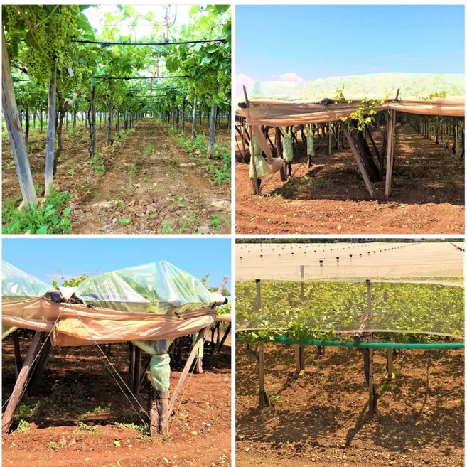
The cultivation of table grapes in Apulia is based on the “overhead” production system (Figure 1), also known in Italian as tendone (meaning “big tent”) because of its characteristic canopy architecture [45]. It is widespread in the Mediterranean region and South America [46], and can be characterized by two types of covers: i) a thin porous plastic net, in order to bring forward the harvest time (from July to June) and decrease the risk of damaging climatic phenomena (hail); and/or ii) a thin plastic film, in order to delay the harvest time (from October to December). The cover modifies
the solar radiation characteristics [47] and hence changes the microclimate (photosynthetically active radiation, air temperature, humidity, and wind speed), plant water status [48–50], gaseous exchanges [51–53], response of the crop to soil water depletion [54], and production yield and quality [55,56]. Furthermore, a vineyard covered by plastic net or film allows a more limited use of irrigation water during the summer, a very important aspect in the Mediterranean area, where water is scarce [57].
Figure 1. Tendone system.
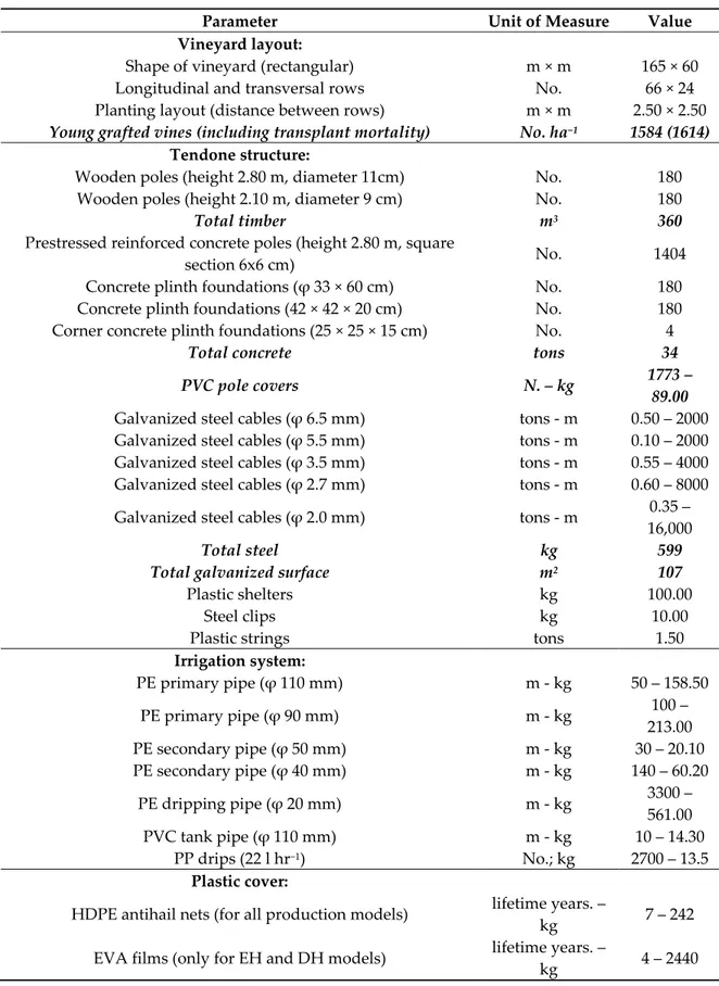
The tendone system is a structure consisting of poles, galvanized steel cables, and plastic nets and/or films. Some poles are made of wood, while others are made of reinforced concrete. The former are fixed in the ground, while the latter have a small foundation. The galvanized steel cables, fixed by anchors in the soil, make a tensile structure that connects each pole to the top and supports the films or nets. Drip irrigation pipes are fixed along the steel cables. The tendone system is constructed through four phases: (i) preliminary operations; (ii) tendone construction; (iii) plastic cover installation; (iv) irrigation system (Table 1).
In Apulia, the most widespread cultivar for table grapes is “Italia”, used in 50% of vineyards, followed by the Victoria, Regina, and Red Globe cultivars. However, in recent years, the rapid spread of seedless varieties, characterized by lower production but higher market prices, has allowed an important supply diversification in terms of cultivar range and harvest time [58].
Table 1. Tendone structure.
Parameter Unit of Measure Value
Vineyard layout:
Shape of vineyard (rectangular) m × m 165 × 60 Longitudinal and transversal rows No. 66 × 24 Planting layout (distance between rows) m × m 2.50 × 2.50
Young grafted vines (including transplant mortality) No. ha−1 1584 (1614) Tendone structure:
Wooden poles (height 2.80 m, diameter 11cm) No. 180 Wooden poles (height 2.10 m, diameter 9 cm) No. 180
Total timber m3 360
Prestressed reinforced concrete poles (height 2.80 m, square
section 6x6 cm) No. 1404 Concrete plinth foundations (ϕ 33 × 60 cm) No. 180 Concrete plinth foundations (42 × 42 × 20 cm) No. 180 Corner concrete plinth foundations (25 × 25 × 15 cm) No. 4
Total concrete tons 34
PVC pole covers N. – kg 1773 –
89.00
Galvanized steel cables (ϕ 6.5 mm) tons - m 0.50 – 2000 Galvanized steel cables (ϕ 5.5 mm) tons - m 0.10 – 2000 Galvanized steel cables (ϕ 3.5 mm) tons - m 0.55 – 4000 Galvanized steel cables (ϕ 2.7 mm) tons - m 0.60 – 8000 Galvanized steel cables (ϕ 2.0 mm) tons - m 0.35 –
16,000
Total steel kg 599
Total galvanized surface m2 107
Plastic shelters kg 100.00 Steel clips kg 10.00 Plastic strings tons 1.50
Irrigation system: PE primary pipe (ϕ 110 mm) m - kg 50 – 158.50 PE primary pipe (ϕ 90 mm) m - kg 100 – 213.00 PE secondary pipe (ϕ 50 mm) m - kg 30 – 20.10 PE secondary pipe (ϕ 40 mm) m - kg 140 – 60.20 PE dripping pipe (ϕ 20 mm) m - kg 3300 – 561.00 PVC tank pipe (ϕ 110 mm) m - kg 10 – 14.30 PP drips (22 l hr−1) No.; kg 2700 – 13.5 Plastic cover:
HDPE antihail nets (for all production models) lifetime years. –
kg 7 – 242 EVA films (only for EH and DH models) lifetime years. –
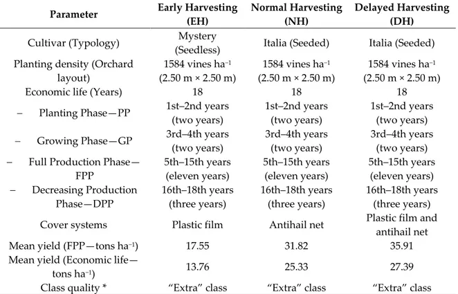
kg 4 – 2440 This study focused on three table grape production models, namely: early harvesting (EH), normal harvesting (NH), and delayed harvesting (DH). Each production model was built and managed in order to cover a different harvesting time, i.e., June, September, and December, respectively (Table 2 and Table 3). The economic life of all the three models in the study area was assumed equal to 18 years, and was divided into four phases:
1. Planting phase (PP), from the first to the second year, in which the vines are not productive and the only economic item is the planting cost;
2. Growing phase (GP), from the third to the fourth year, in which vines and production grow, so that revenues increase more than proportionally compared to costs;
3. Full production phase (FPP), from the fifth to the fifteenth year, in which vine growth is complete and production is stable, so that revenues and costs are constant;
4. Decreasing production phase (DPP), from the sixteenth to the eighteenth year, in which vine ageing reduces the production, so that revenues decrease more than proportionally compared to costs.
The accurate identification of all the life stages of the tendone system is necessary due to its changeable levels of inputs and outputs (Tables A1–A3), as well as of costs and revenues, during the economic life [12,59]. The yields for the three models considered vary from zero (PP) to a maximum of 18 t ha−1, 32.5 t ha−1, and 37 t ha−1 in the FPP phase of the EH, NH, and DH models, respectively
(Figure 2). The extirpation of the vineyard takes place at the end of the eighteenth year, when the productivity is 50% lower compared to the FPP phase. Therefore, the average annual productivity during the economic life of the vineyard is 25.33 t ha−1 y−1 for the NH model, 13.76 t ha−1 y−1 for the
EH model, and 26.10 t ha−1 y−1 for the DH model. These differences are due to both the variation of
the harvesting time and to the cultivar.
Table 2. Main futures of the three production models.
Parameter Early Harvesting
(EH)
Normal Harvesting (NH)
Delayed Harvesting (DH)
Cultivar (Typology) Mystery
(Seedless) Italia (Seeded) Italia (Seeded) Planting density (Orchard
layout)
1584 vines ha−1 1584 vines ha−1 1584 vines ha−1
(2.50 m × 2.50 m) (2.50 m × 2.50 m) (2.50 m × 2.50 m) Economic life (Years) 18 18 18
Planting Phase—PP 1st–2nd years 1st–2nd years 1st–2nd years (two years) (two years) (two years)
Growing Phase—GP 3rd–4th years 3rd–4th years 3rd–4th years (two years) (two years) (two years)
Full Production Phase— FPP
5th–15th years 5th–15th years 5th–15th years (eleven years) (eleven years) (eleven years)
Decreasing Production Phase—DPP
16th–18th years 16th–18th years 16th–18th years (three years) (three years) (three years) Cover systems Plastic film Antihail net Plastic film and
antihail net Mean yield (FPP—tons ha−1) 17.55 31.82 35.91
Mean yield (Economic life—
tons ha−1) 13.76 25.33 27.39
Class quality * “Extra” class “Extra” class “Extra” class
Figure 2. Production periods of the three table grape vineyards.
The Mystery cultivar for the EH model and the Italia cultivar for the NH and DH models were considered, i.e., the most widespread and suitable cultivars in the study area (in the Apulia region, neither the Italia Cultivar or other cultivars containing seeds are cultivated according to the EH model that, instead, is mainly based on seedless cultivars (for example, Mystery)). Consequently, yield per hectare varies among models, namely it increases from EH to DH. In any case, the “extra” class quality for all models was assumed.
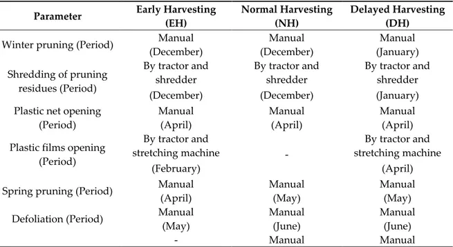
The farming practices for the three models are summarized in Table 3. Pruning (in winter and spring) is performed manually. In contrast, a tractor equipped with various implements allows the following operations: shredding of pruning residues by a wood grinder; removal of weeds and ploughing through a milling machine, plough, or tiller; distribution of fertilizers by a manure spreader; pest control by an atomizer. Irrigation water is collected by aquifer with a pump that injects water into the pipes and drips.
Table 3. Main farming practices for the three production models.
Parameter Early Harvesting (EH)
Normal Harvesting (NH)
Delayed Harvesting (DH)
Winter pruning (Period) Manual Manual Manual (December) (December) (January) Shredding of pruning residues (Period) By tractor and shredder By tractor and shredder By tractor and shredder (December) (December) (January) Plastic net opening
(Period)
Manual Manual Manual (April) (April) (April) Plastic films opening
(Period) By tractor and stretching machine - By tractor and stretching machine (February) (April) Spring pruning (Period) Manual Manual Manual
(April) (May) (May) Defoliation (Period) Manual Manual Manual
(May) (June) (June) - Manual Manual
Small acini detachment
(Period) (June) (June)
Winter fertilization with granular chemical fertilizers (Period)
By spreader By spreader By spreader (February) (February) (February) Fertirrigation technique
with liquid chemical fertilizers (N. of interventions and
period)
Drip irrigation Drip irrigation Drip irrigation (2 times year 1, May–
June)
(2 times year 1, May– June)
(2 times year 1, May– June) Irrigation technique (N.
of interventions and period)
Drip irrigation Drip irrigation Drip irrigation (2 times year 1, May–
June)
(4 times year 1, May– July)
(5 times year 1, May– September)
Weed control (Period)
Mechanical tillage and herbicides spread by tractor and
atomizer
Mechanical tillage and herbicides spread by tractor and
atomizer
Mechanical tillage and herbicides spread by tractor and
atomizer (February–July) (April–July) (February–
September)
Pest control (Period, Frequency)
Conventional technique using tractor and atomizer
Conventional technique using tractor and atomizer
Conventional technique using tractor and atomizer (April–May, Weekly) (April–August,
Weekly)
(April–November, Weekly) Harvest method (Period) Manual Manual Manual (June) (September) (December) Plastic net closing
(Period)
Manual Manual Manual (September) (October) (January) Plastic films closing
(Period) By tractor and stretching machine - By tractor and stretching machine (September) (January) 2.1.2. Functional Units and System Boundaries
The functional unit (FU) is the unit of agricultural area cultivated for 18 years (1 ha). Furthermore, for comparison among the three production models, 1 t ha−1 y−1 is also used, namely 1
ton of table grapes produced on one hectare of cultivation for an average annual production, calculated by including all the phases of the economic life of the vineyard.
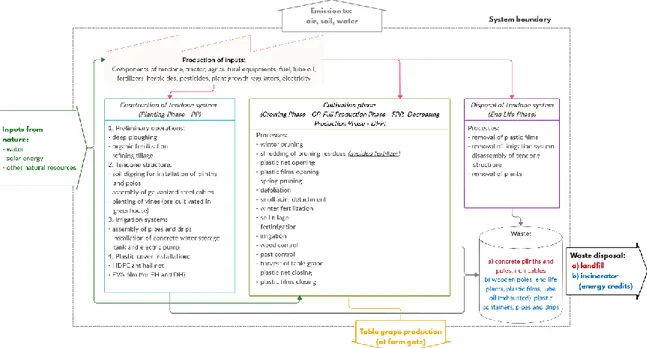
The processes and materials used for the construction of the tendone system (Table 1) were considered as part of the system boundaries (Figure 3). The soil preparation consists of a deep ploughing, organic fertilization, and refining tillage. These operations, evaluated per hectare of land, are carried out through a tractor that operates with the use of diesel and lube oil. All the agricultural machines, consumption, maintenance, and production energy were evaluated and preset in the LCA software used (Gabi ver. 8) [60]. The housing of the tractor is a shed.
Figure 3. Flow chart of the tendone system.
The construction of the tendone requires a soil digger for plinths and anchors, concrete precasts support pole (lifetime 36 years), plinths (lifetime 36 years), wooden poles (lifetime 18 years), galvanized steel cables (lifetime 36 years), and table grape seedlings. In addition, the irrigation system is installed and it is made of: plastic pipe with drippers (lifetime 4 years); plastic water storage tank (lifetime 36 years); electric pump. The materials of the irrigation system are: plastic tanks (HDPE), pipes with drip (LDPE), electrically powered hydraulic pump. The tubes ϕ 20 are replaced every four years due to the obstruction of the drippers. The other pipes have a life time of 18 years. The electrical consumption of the pump is modelled based on power and hydraulic prevalence [60]. The seedlings are produced in unheated greenhouses and are counted with an excess of 3% to consider the mortality in the transplant.
The plastic covering materials and antihail nets are positioned on the tendone and fixed to the steel cables by means of plastic strings. High-density polyethylene (HDPE) antihail nets and ethylene–vinyl acetate (EVA) have a lifetime of 9 and 4 years, respectively. The quantities used are shown in the Table 1.
The agrochemicals considered in the analysis were divided in the following groups: insecticides, herbicides, fungicides, and growth regulators (Tables A1–A3). All agrochemicals were evaluated for their production and distribution. For their dispersion in the soil and in the environment, the Usetox 2.1 software [61] based on the Mackay model [62]) was used. Agrochemicals are applied using a field sprayer whose consumption is parameterized based on 1 hectare of cultivated area. Regarding the production of fertilizers, we implemented the processes in Gabi (ver. 8) [60], by means of the fertilizer calculator present in the software when the fertilizers are not in these databases or the concentrations of N, P2O5, and K2O do not coincide with those of the products used. The fertilizers obtained are
expressed as the sum of: ammonia (liquid), potassium chloride (60% K2O), and raw phosphate (32.4%
P2O5). Emissions of nitric and ammonia nitrogen and phosphates present in the soil and water,
released fertilizers, were quantified by deducting the percentage spread in the air as NH3, N2O, and
NOx from the concentrations encountered in the DOP analysis [63,64]. The remaining rate was
considered available for crops (considering also the nitrogen present in the soil) but 20% of the remaining amount, in the case of clay soils, can be considered percolated in groundwater [65]. N2O
emissions into the air from any source were processed according to the formula proposed by Bouwman [66]. The nutrients removal by the vines were deducted from literature data [67].
The emission model SALCA-P [68]) was used for phosphorus emissions, such as leaching of soluble phosphate (PO4) to ground water and run-off of soluble phosphate to surface water. The
heavy metal emissions were calculated by SALCA-heavy metal [69,70]). Inputs into farm soil and outputs to surface water and groundwater were calculated based on heavy metal input from fertilizers and agrochemicals. The pruning residues were considered a coproduct since they were shredded into the soil. Therefore, they were considered as avoided fertilizer.
The machineries used for the cultivation practices were simulated through a “generic agricultural machine” based on weight. The transport of all the components necessary for the construction of the tendone system were hypothesized on trucks for a distance of 40 km. Tractor and agricultural machinery transport were neglected.
We assumed that end of life of the plastic covering materials (plastic nets/films), pole covers and strings, wooden poles, and the biomass produced by the grapevine’s plants removed after 18 years involved transport for 100 km to an incinerator with energy recovery and consequent combustion, due to the contamination with agrochemicals. The electricity produced by these wastes in the incinerator was deducted from consumption for the production cycle. In addition, we assumed that end of life of the steel cables, prestressed concrete piles, and foundations involved transport for 100 km to a collection center for building materials.
Land use was estimated using indicators of both land occupation and transformation. In this study, transformation (from and to) were introduced by considering biodiversity depletion [71]. Mineral extraction was characterized considering some additional resources and water in the soil, derived from the minerals category of the Ecoindicator 99 method [71]. For the radioactive waste category, generated by a nuclear plant in the electricity mix, the characterization and normalization factors of the EDIP 2003 method [72] were carried out.
2.1.3. Evaluation Method and Impact Categories
Gabi (version 8) [60] with the support of the Ecoinvent 3.3 [73] database was used for the analysis. Moreover, the UseTox 2.1 software [61] was used for calculation of both the distribution coefficients of the pesticides in the environmental compartments and the relative values of the characterization factors of these substances.
For the FU of 1 ha, the IMPACT 2002+ method was used. This method provided 15 midpoint impact and 4 endpoint damage assessment categories. Furthermore, it included more substances than other LCA analysis methods [74]. IMPACT 2002+ was a combination of four methods: IMPACT 2002 [75], Eco-indicator 99 [76], CML [77]), and IPCC [64]. This evaluation method represents an effort to combine/harmonize midpoints and endpoints. The endpoint indicators, based on the aggregation of the midpoint ones, allow a more attractive and understandable information. In addition, through the damage characterization factors of the reference substances, the endpoint indicators account the synergies among the substances of the inventory.
The results concerning the FU of 1 tontg ha−1 y−1, on the other hand, were obtained through the CML
2001 method, version 2015 [78]. Indeed, the IMPACT 2002+ method for this FU was of scarce interest, since its results can be calculated by the ratio between the results related to the FU of 1 ha and the yield of each production model.
2.2. LCC Analysis
LCC methodology was used to assess and compare the economic profile of the three production models considered. LCC, jointly to LCA, can improve the decision-making processes [27], however, despite being the first life cycle analysis tool to be developed, it has not yet been standardized by specific norms, except for the building sector [79]. However, in this study, a conventional LCC analysis [79] based on financial indicators was carried out.
The suitability and implementation of investments are affected by several financial characteristics, i.e., cash flows, time value of money, risk, return, and maximization of profits [80]. Several methods concerning the capital budgeting allow the assessment of one or more of these financial characteristics [81]. However, each method is affected by specific weaknesses, so that the synergic use of these tools is a recommended practice in the economic literature [82] to evaluate the effectiveness and efficacy of investments. In the present study, the following capital budgeting indexes were used: net present value
(NPV), internal rate of return (IRR), discounted benefit–cost rate (DBCR), and discounted payback time (DPBT).
NPV [83,84]) is a long-term assessment index of investments’ magnitude. This index investigates the implications of one or more future investments, allowing also the selection of the best one under given market conditions [85]. This index is calculated by the difference between the discounted annual revenues (cash inflows) and the discounted annual costs (cash outflows), i.e.,:
𝑁𝑃𝑉 = ∑𝑅𝑡− 𝐶𝑡 (1 + 𝑟)𝑡 𝑛
𝑡=0
(1)
where NPV is the net present value; R and C represent the discounted annual revenues and the discounted annual costs, respectively; t is the cash flow time; n is the investment time span; and r is the discount rate. A positive NPV indicates that the investment is convenient. In the presence of two or more alternative investments, the highest NPV value identifies the most profitable option. This approach is risk-adjusted, unlike other indicators such as IRR, given that riskier investments are expected to generate higher returns [86].
IRR [87] measures the profitability and efficiency of investments by discounting the rate r up to zero the NPV [88]:
∑ 𝑅𝑡−𝐶𝑡 (1+𝑟)𝑡 𝑛
𝑡=0 = 0. (2)
If the IRR is higher than the prefixed reference rate, an investment is profitable [89]. In addition, the best of alternative investments is the one with the highest IRR.
DBCR is the ratio between the discounted annual revenues from the investment life span and the corresponding discounted annual costs [90]:
𝐷𝐵𝐶𝑅 =∑𝑛𝑡=0𝑅𝑡/(1+𝑟)𝑡
∑𝑛𝑡=0𝐶𝑡/(1+𝑟)𝑡. (3)
The investment is convenient if the ratio is greater than one; given several investments, the one with the highest ratio should be preferred [91].
DPBT measures the period (i.e., number of years) at the end of which the cumulative discounted cash flows equal the investment costs [92]. Therefore, an investment becomes more viable with the decreasing of the ratio.
Since medium- and long-term currency values and technical innovation generate fluctuations of investments, a Monte Carlo analysis was applied in order to avoid the determinism of the financial indicators and to evaluate economic and technical risks [93–95]. In particular, 1000 sets of cash flows using a normal distribution for four periods were generated (1–2, 3–4, 5–15, 16-18 years), with the mean and standard deviation obtained from the sample data. Indeed, the analysis based on specific investment periods was justified by the heterogeneity of their respective cash flows (i.e., negative, increasing, constant, and decreasing), thus preventing investment results from a single probability distribution. Finally, for each production model, the averages were calculated from the 1,000 sets generated for each period.
The LCC analysis was based on the following assumptions:
The annual total costs were evaluated at current prices. The total costs include specific costs (fertilizers, pesticides, irrigation water, fuel and lubricants, power) and other nonspecific operating costs concerning labor and mechanical operations, which were assessed considering the current hourly wage of workers for the manual operations and the current tariffs charged by agricultural service providers for the mechanical operations, respectively [44];
The annual total revenues included the revenue from selling the table grapes, but excluded the Common Agricultural Policy (CAP) direct aids [44];
The discount rate was set at 4% considering alternative but similar investments in terms of type, market conditions, duration, and risk [96];
The revenues per production model were calculated considering the average of farm gate prices on the marketplace of Bari (Italy) during the last five years, i.e., between 2014–2018 [2], namely 0.90
€/kg for the Mystery cultivar in the EH model, 0.55 €/kg for the Italia cultivar in the NH model, and 0.70 €/kg for the Italia cultivar in the DH model;
Annual inflows and outflows were calculated assuming constant financial conditions over the entire 18-year period [97,98].
Primary data for the LCC analysis concerned the revenues and costs referred to each year of the economic life of the three vineyards considered and, as for the LCA, were validated through a panel of experts operating in the study area.
3. LCA Results
3.1. Life Cycle Impact Assessment (LCIA): Midpoint Analysis
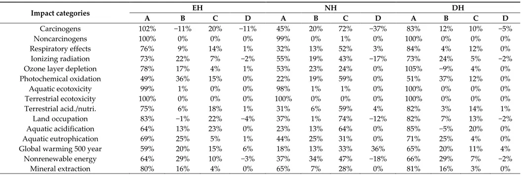
The LCIA results of midpoint analysis (Table 4) highlighted that the NH model generated the smallest environmental impacts for each impact category assessed, followed by the EH and DH models. Furthermore, the percentage impact of emissions related to the main phases constituting the production process was assessed (Table 5), namely: (A) cultivation practices, concerning tillage, irrigation, etc. and based on the use of inputs (agrochemical, fertilizers, etc.); (B) use of coverings materials (plastic films and nets) and disposal to incinerator, with calculation of energy credits; (C) tendone construction and final disposal of its components (concrete and iron cable) to landfill; (D) disposal of the final vineyard biomass in a municipal incinerator, with calculation of energy credits. Noteworthy are the energy credits, which can cause negative contributions.
The results highlighted that, in the EH model, all the impact categories were mainly affected by the cultivation practices. In particular, the production and use of fertilizers caused the following most important emissions per impact category (in brackets): zinc into soil (noncarcinogens); fine particles into air (respiratory effects); halon 1211, generated by production of caum nitrate, into air (ozone layer depletion); non-methane volatile organic compounds (NMVOC) into air (photochemical oxidation); copper into soil (aquatic ecotoxicity); zinc into soil (terrestrial ecotoxicity); ammonia into air (terrestrial acidification/nutrification); sulphur dioxide into air (aquatic acidification); phosphates into water (aquatic eutrophication); natural gas consumption (nonrenewable energy); nickel consumption (mineral extraction). In addition, the electricity use for irrigation causes the following emissions: NMVOC into air and molybdenum into water (carcinogens), C14 into air (ionizing radiation), halogenated halon 1301 and R-114 (ozone layer depletion), sulphur dioxide and CO2 into
air (global warming).
The cultivation practices generated the highest impacts in the NH model too. In particular, the most important impact categories were: noncarcinogens, ionizing radiation, ozone layer depletion, aquatic ecotoxicity, terrestrial ecotoxicity, aquatic eutrophication, and mineral extraction. The production and use of fertilizers caused the greatest emissions, due to zinc into soil (noncarcinogens), NMVOC group into air (ozone layer depletion), copper into soil (aquatic ecotoxicity), zinc in the soil (terrestrial ecotoxicity), phosphates into water (aquatic eutrophication), and consumption of nickel (mineral extraction). The use of electricity for irrigation caused the most important emissions due to Radon 222 (ionizing radiation). The construction of the tendone system mainly influenced the following impact categories: carcinogens, respiratory effects, photochemical oxidation, terrestrial acidification/nutrification, aquatic acidification, and nonrenewable energy. More specifically, the production of PVC parts (strings and pole cover) caused the higher emissions of NMVOC into air (carcinogens, but compensated by the energy credits that avoid the emission of dioxins; photochemical oxidation) and natural gas consumption (nonrenewable energy). The galvanization of steel cables produced emissions of fine dust (respiratory effects), nitrogen oxides, and monoxide (terrestrial acidification/nutrification), and ammonia (aquatic acidification). Finally, the production of concrete caused the greatest CO2 emissions (global warming), which were balanced by the energy
credits from the disposal of final biomass.
Lastly, the cultivation practices mainly affected all the impact categories in the DH model too. In particular, the use and production of fertilizers caused emissions of zinc into soil (noncarcinogens), fine particles into air (respiratory effects), halon 1211 into air (ozone layer depletion), NMVOC into
air (photochemical oxidation), copper into soil (aquatic ecotoxicity), zinc into soil (terrestrial ecotoxicity), ammonia into air (terrestrial acidification/nutrification), phosphates into water (aquatic acidification), and nickel consumption (mineral extraction). The use of electricity for irrigation caused NMVOC into air (carcinogens), C14 into air (ionizing radiation), CO2 into air (global warming 500
year), natural gas consumption (nonrenewable energy).
For the three production models, the land use category depended on the transformation and occupation of agricultural land, and, specifically for the EH and DH models, there was an increase due to a proportional use of fertilizers and electricity to consumption.
In summary, the LCIA showed that the greatest environmental loads come from:
Irrigation and production/use of fertilizers in the cultivation phase;
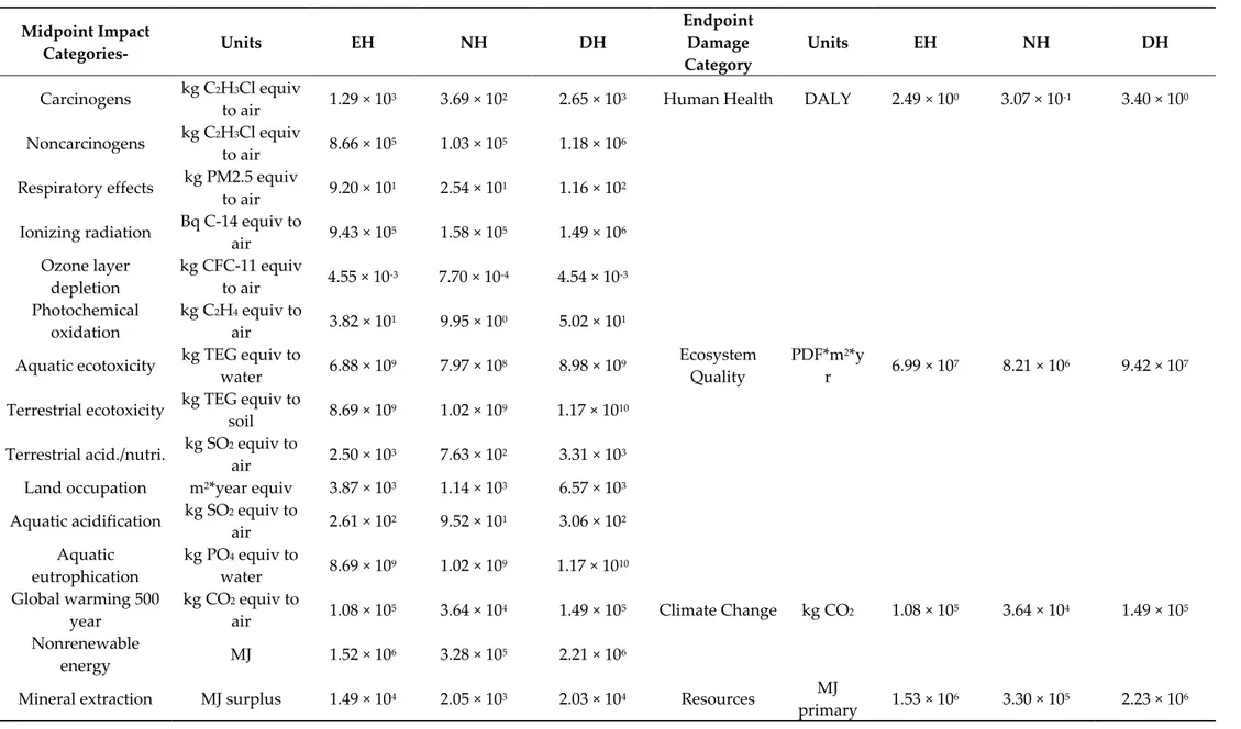
Table 4. LCIA results for table grape production related to the functional unit of 1 ha of cultivated area: midpoint results from characterization analysis and endpoint
results from damage assessment (Impact 2002+).
Midpoint Impact Categories- Units EH NH DH Endpoint Damage Category Units EH NH DH Carcinogens kg C2H3Cl equiv
to air 1.29 × 10³ 3.69 × 10² 2.65 × 10³ Human Health DALY 2.49 × 100 3.07 × 10⁻¹ 3.40 × 100 Noncarcinogens kg C2H3Cl equiv
to air 8.66 × 10
5 1.03 × 10⁵ 1.18 × 10⁶
Respiratory effects kg PM2.5 equiv
to air 9.20 × 101 2.54 × 101 1.16 × 10² Ionizing radiation Bq C-14 equiv to
air 9.43 × 10 5 1.58 × 10⁵ 1.49 × 10⁶ Ozone layer depletion kg CFC-11 equiv to air 4.55 × 10⁻³ 7.70 × 10⁻⁴ 4.54 × 10⁻³ Photochemical oxidation kg C2H4 equiv to air 3.82 × 10 1 9.95 × 100 5.02 × 101
Aquatic ecotoxicity kg TEG equiv to
water 6.88 × 10⁹ 7.97 × 10⁸ 8.98 × 10⁹
Ecosystem Quality
PDF*m2*y
r 6.99 × 10⁷ 8.21 × 10⁶ 9.42 × 10⁷ Terrestrial ecotoxicity kg TEG equiv to
soil 8.69 × 10
9 1.02 × 10⁹ 1.17 × 10¹⁰
Terrestrial acid./nutri. kg SO2 equiv to
air 2.50 × 10³ 7.63 × 10² 3.31 × 10³ Land occupation m2*year equiv 3.87 × 10³ 1.14 × 10³ 6.57 × 10³
Aquatic acidification kg SO2 equiv to
air 2.61 × 10 2 9.52 × 101 3.06 × 10² Aquatic eutrophication kg PO4 equiv to water 8.69 × 10⁹ 1.02 × 10⁹ 1.17 × 10¹⁰ Global warming 500 year kg CO2 equiv to air 1.08 × 10 5 3.64 × 10⁴ 1.49 × 10⁵ Climate Change kg CO2 1.08 × 10⁵ 3.64 × 10⁴ 1.49 × 10⁵ Nonrenewable energy MJ 1.52 × 10⁶ 3.28 × 10⁵ 2.21 × 10⁶
Mineral extraction MJ surplus 1.49 × 10⁴ 2.05 × 10³ 2.03 × 10⁴ Resources MJ
primary 1.53 × 10
Table 5. The percentage incidence on the midpoint impact categories for each grape model phase (Impact 2002+). Impact categories EH NH DH A B C D A B C D A B C D Carcinogens 102% −11% 20% −11% 45% 20% 72% −37% 83% 12% 10% −5% Noncarcinogens 100% 0% 0% 0% 99% 0% 1% 0% 100% 0% 0% 0% Respiratory effects 76% 9% 14% 1% 32% 13% 52% 3% 84% 4% 12% 0% Ionizing radiation 73% 22% 7% −2% 55% 19% 43% −17% 73% 24% 5% −2% Ozone layer depletion 78% 17% 4% 1% 53% 23% 24% 0% 105% −9% 4% 0% Photochemical oxidation 49% 36% 15% 0% 22% 19% 59% 0% 51% 37% 12% 0% Aquatic ecotoxicity 99% 1% 0% 0% 98% 1% 1% 0% 100% 0% 0% 0% Terrestrial ecotoxicity 100% 0% 0% 0% 100% 0% 0% 0% 100% 0% 0% 0% Terrestrial acid./nutri. 75% 6% 18% 1% 31% 6% 59% 4% 82% 3% 14% 1% Land occupation 83% −1% 22% −4% 37% 1% 74% −12% 82% 7% 13% −2% Aquatic acidification 64% 13% 23% 0% 23% 13% 64% 0% 85% −5% 20% 0% Aquatic eutrophication 69% 25% 5% 1% 44% 25% 31% 0% 71% 25% 4% 0% Global warming 500 year 59% 20% 15% 6% 18% 13% 33% 36% 65% 20% 11% 4% Nonrenewable energy 64% 29% 10% −3% 37% 34% 47% −18% 66% 29% 7% −2%
Mineral extraction 80% 16% 4% 0% 65% 7% 28% 0% 81% 16% 3% 0%
A—cultivation practices; B—use of covering materials and disposal (energy recovery); C—tendone construction and disposal; D—disposal of final vineyard biomass (energy recovery).
3.2. Life Cycle Impact Assessment (LCIA): Endpoint Analysis
Regarding the results of LCIA at the endpoint (Table 5), the human health, ecosystem quality, climate change, and resources indices all had the same trend with the highest damage values obtained from the DH production model, followed by the EH model and the NH production model. This was due to the greater use of plastic materials and the greater use of resources for the EH and NH cultivation cycles.
The following remarks can be made for all the three production models. For the human health index, the greatest contribution came from the ionizing radiation category and therefore from the use of electricity for irrigation. For the ecosystem quality index, the greatest contribution was provided by the terrestrial ecotoxicity category and therefore by the use of fertilizers. The resources index was influenced by the nonrenewable energy category, which depends on the use of electricity for irrigation. The climate change index was influenced by the use of electricity for irrigation like the global warming category, for the EH and DH production models. The same index was mainly influenced by the final disposal with incineration of the wood biomass and by the use of concrete for the NH production model.
3.3. LCA Results Related to the Functional Unit of 1 Ton of Table Grape
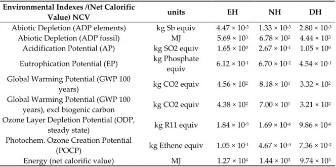
The results concerning the FU of 1 tontg ha−1 y−1 (Table 6), based on the CML2001 evaluation
method (ver.2016) but with the exclusion of the toxicity indices, highlighted that the NH model had the lowest environmental load, the EH model generated the worse performance, and the DH model had intermediate effects. Furthermore, compared to the NH model, the environmental loads of the DH model were 1.9 times (ADP el. index)—5.9 times (EP index) greater, while the impacts of the EH model were 1.3 times (ADP el. index)—4.7 times (EP index) greater.
Noteworthy is that these results were affected by the diverse yields of the three models considered (high for the DH, intermediate for the NH, and low for the EH model). Indeed, the NH and the DH models were based on the Italia cultivar, whereas the EH model used the Mystery cultivar. However, the comparison remained consistent when considering the commercial strategy put in place by farmers of the study area, since the Italia cultivar is not suitable for early production, and vice versa.
Table 6. Results of the life cycle assessment (LCA) analysis on the production of table grapes related
to the functional unit 1 tontg ha−1 y−1 (CML 2001).
Environmental Indexes /(Net Calorific
Value) NCV units EH NH DH
Abiotic Depletion (ADP elements) kg Sb equiv 4.47 × 10⁻³ 1.33 × 10⁻³ 2.80 × 10⁻³
Abiotic Depletion (ADP fossil) MJ 5.69 × 10³ 6.78 × 10² 4.44 × 10³
Acidification Potential (AP) kg SO2 equiv 1.65 × 100 2.67 × 10⁻¹ 1.05 × 100
Eutrophication Potential (EP) kg Phosphate
equiv 6.12 × 10
-1 6.70 × 10⁻² 4.54 × 10⁻¹
Global Warming Potential (GWP 100
years) kg CO2 equiv 4.56 × 10² 8.18 × 101 3.32 × 10² Global Warming Potential (GWP 100
years), excl biogenic carbon kg CO2 equiv 4.38 × 10
2 7.00 × 101 3.21 × 10²
Ozone Layer Depletion Potential (ODP,
steady state) kg R11 equiv 1.84 × 10⁻⁵ 1.69 × 10⁻⁶ 9.86 × 10⁻⁶ Photochem. Ozone Creation Potential
(POCP) kg Ethene equiv 1.05 × 10
-1 4.67 × 10⁻³ 7.36 × 10⁻²
3.4. LCC Results
3.4.1. Financial Analysis
The economic performance of the three table grape models was evaluated thorough the life cycle costing methodology, estimating the following indexes: net present value (NPV), internal rate of return (IRR), discounted benefit–cost rate (DBCR), and discounted payback time (DPBT). The results are summarized in Table 7.
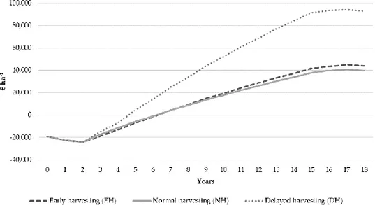
In terms of cumulative discounted cash flows (Figure 4):
The DH model had the best financial performance;
The EH and NH models had similar performance, but lower compared to the DH model. In particular, the three production models were comparable during the two years of the planting phase. Subsequently, their performances tended to diverge. Even with a minimum difference compared to the NH model, the EH model showed lower cumulative discounted cash flows between the second and the sixth year, which tended to equalize in the seventh year. Thus, starting from the eighth year, the performance of the EH model was better than the NH model. The cumulative discounted cash flows of the DH model, on the other hand, increased more starting from the growing phase and generated a difference of roughly 50,000 € ha−1 at the end of the economic life of the
vineyard.
These significant differences were mainly the joint effect of the discrepancy between both the market price of table grapes and the yields of the cultivars considered. Indeed, even if the EH model can exploit the highest unit production value (0.90 € kg−1) and the lowest costs, its lower yield
generates a financial performance over 18 years that is comparable to the NH model. In contrast, even if the DH model is characterized by the highest costs and average market price of production (0.70 € kg−1), its global financial performance is significant. These first results highlighted that the financial
viability of the EH model is similar to the NH model; on the contrary, the differentiation of the harvesting time ensures significantly higher profits than the NH model, which makes sense for the DH model.
Figure 4. Cumulative discounted cash flows of the three production models.
The Monte Carlo approach confirmed these findings (Table 7). Indeed, the DH model was characterized by the highest NPV, IRR, and DBCR, and by the lowest DPBP. In contrast, the EH and NH models indicated a lower viability for farmers to implement these production models. Furthermore, their performances were very similar, so it should be considered to what extent management of the EH model could benefit farmers compared to the NH model. These findings make it possible to argue that the greater costs related to the use of the plastic net are not completely justified by the market, though the EH model allows a lower use of inputs due to the shorter duration
of the growing cycle. In contrast, the DH model, based on a higher use of inputs during a longer growing cycle, is justified by the table grape market due to the higher profits.
Table 7. Life cycle costing (LCC) results from the Monte Carlo analysis.
Production models NPV IRR DBCR DPBP
EH 42,104.77 18.6% 1.38 8.56 NH 37,222.38 12.7% 1.26 8.15 DH 94,372.16 31.2% 1.74 5.14 3.4.2. Sensitivity Analysis
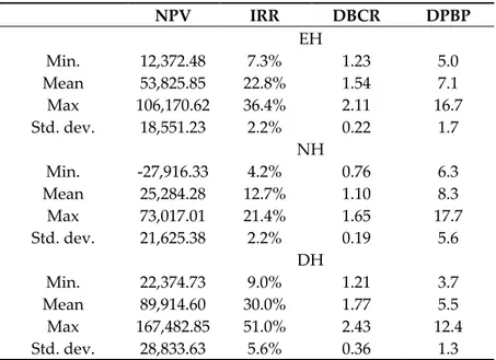
A sensitivity analysis of price and cost variations was carried out in order to study the differences in the financial parameters due to fluctuations in market conditions. The above economic items varied between −20% and +20%, below and above the baseline values (Table 8). This range was set, taking into account the volatility of farm gate prices and production factors foreseeable in the market with current economic conditions [99,100].
These results allowed a deeper reflection on the viability of the three production models, since selling price and cost variations significantly influenced the economic viability of the investments. In particular, the simulations confirmed the greater viability of the DH model, whose financial indicators indicated the best performance. Furthermore, the analysis shed light on the real viability between the EH and the NH models. The former was characterized by values of the financial indicators at least 28% higher than the NH model for the NPV, IRR, and DBCR indicators, and at least 5% lower for the DPBP indicator. Therefore, it is possible to argue that, in terms of financial performance, the DH model is the best one, followed by the EH model and lastly by the NH model.
Table 8. Sensitivity analysis results.
NPV IRR DBCR DPBP EH Min. 12,372.48 7.3% 1.23 5.0 Mean 53,825.85 22.8% 1.54 7.1 Max 106,170.62 36.4% 2.11 16.7 Std. dev. 18,551.23 2.2% 0.22 1.7 NH Min. -27,916.33 4.2% 0.76 6.3 Mean 25,284.28 12.7% 1.10 8.3 Max 73,017.01 21.4% 1.65 17.7 Std. dev. 21,625.38 2.2% 0.19 5.6 DH Min. 22,374.73 9.0% 1.21 3.7 Mean 89,914.60 30.0% 1.77 5.5 Max 167,482.85 51.0% 2.43 12.4 Std. dev. 28,833.63 5.6% 0.36 1.3 4. Discussion of Results
The environmental analysis highlighted that the NH model generated the lowest environmental load, followed by the EH and DH models, for all the indexes considered. Furthermore, with respect to the unit function of 1 ton of table grapes, the EH model caused the greatest environmental loads (Table 6) and provided a slight improvement in the economic results (Figure 4). From the financial analysis, on the other hand, it emerged that the DH model is the most profitable, followed by the EH and NH models. Therefore, compared to the NH model, the DH model has a higher environmental burden but also a higher economic performance, while the EH model is not fully justified due to its
worse environmental results and similar economic viability. Thus, for the three models considered, a certain divergence exists between environmental and economic impacts.
However, in the real world, the three production models coexist in specialized table grape farms with the aim of covering the entire harvesting period (from June to December). Indeed, the coexistence of different production models is due to a management strategy aimed at reducing the market risk deriving from the volatility of table grape prices and expanding the farming work schedule, with positive repercussions on productive factor efficiency. Thus, considering that the management of the three production models is necessary for farmers, certain technical solutions should be implemented in order to reduce the environmental burden deriving from the table grape cultivations. Indeed, the results of the environmental analysis highlighted certain hot spots. In the construction of the tendone system, for example, galvanizing the cables has a significant impact and therefore polyamide cables could be used as an alternative. For concrete or wooden poles, a possible alternative is to experiment with elements made of recycled plastic, with a mesh shape and/or reinforced with nongalvanized steel.
For the cultivation phase, on the other hand, the use of power for irrigation, and chemical fertilizers and agrochemicals have a particularly significant impact, and therefore energy could be produced from renewable sources and organic rather than chemical fertilizers could be used [101]. The use of agrochemicals is, on the other hand, the most serious problem. The primary data highlighted about 26 applications based on several molecules. In addition, cases of soil fatigue were reported from the information gathered.
5. Conclusions
This study proved the existence of relevant tradeoffs between environmental and economic performance in the Italian table grape sector. In addition, results showed the main determinants of the environmental impacts and economics returns for each of the investigated production models. However, findings of the analysis could not be exhaustive because of some limitations. The first is due the assumption of LCA concerning system boundaries. The extension of the system boundaries behind the farm gate, by including the conditioning (cooling, sulfuration, packing, cold storage) and transportation phases could be relevant, in particular for the product exported. Indeed, transportation of fresh products for long distances could have a very high environmental impact [6]. In addition, the assumptions of LCC analysis (i.e., the flow costs, prices, yields, and discount rate among the lifetime of production models) affected the results, though the sensitive analysis mitigated this shortcoming. Also, the relation between some productive parameters of the three production models, i.e., yields and quality of grapes, should be further investigated [102,103]. Finally, the availability of more farm case studies would increase the accuracy of the estimate, in terms of their representativeness of table grapes sector at national scale.
Further research is needed to find innovative solutions to enhance the environmental sustainability of the surveyed production models. Although the use of degradable plastics has been the subject of several research projects, currently there are no products with mechanical performance and durability that can replace conventional plastics for the protection of table grape vineyards. Moreover, the performance of some innovative cultivation methods should be evaluated, such as the cultivation of vines in soilless greenhouses opened during the winter [104,105] or the cultivation under high tunnels [106]. Finally, the comparison between conventional and organic production models should ascertain if the conversion of farms to organic method is a viable strategy to improve the overall sustainability, similarly to other fruit sectors [107,108]
Author Contributions: Conceptualization, L.R., A.C., G.R., B.C.d.G., and R.S.; LCA methodology, G.R. L.R., and
R.S.; LCC methodology, R.S. and L.R.; data survey, A.C., L.R., G.R., B.C.d.G., and R.S.; formal analysis, L.R., R.S., and G.R.; writing—original draft preparation, L.R., R.S., and G.R.; supervision, L.R., A.C., amd B.C.d.G. All authors have read and agreed to the published version of the manuscript.
Funding: This research received no external funding.
Appendix A
Table A1. Inputs and outputs of early harvesting (EH) model during the life cycle (18 years).
INPUT Short Description Unit of Measure Construction of Tendone System Planting Phase—PP Growing Phase—GP Full Production Phase—FPP Decreasing Production Phase—DPP Disposal of Tendone Total Fungicides (as
active principle): Penconazole g - 0.00 240.00 1980.00 450.00 - 2670.00
Cyproconazole g - 0.00 160.00 1760.00 480.00 - 2400.00 Dimetomorf g - 0.00 400.00 2200.00 600.00 - 3200.00 Myclobutanil g - 0.00 42.00 462.00 63.00 - 567.00 Metalaxyl-m g - 200.00 200.00 1100.00 300.00 - 1800.00 Copper g - 1419.00 1419.00 7804.50 2128.50 - 12,771.0 0 Insecticides: Methiocarb g - 3604.00 3604.00 19,822.00 5406.00 - 32,436.0 0 Chlorpyrifos-methyl g - 1605.60 3211.20 22,077.00 4816.80 - 31,710.6 0 tau-Fluvalinate g - 0.00 512.00 2,816.00 768.00 - 4096.00 Plant growth regulators: Cytokin l - 0.00 1.00 5.50 1.50 - 8.00 Gibberellins g - 0.00 16.00 88.00 24.00 - 128.00
Fertilizers: Nitric nitrogen kg 0.00 0.00 30.48 167.64 45.72 - 243.84
Ammoniacal nitrogen kg 0.00 0.00 1.32 7.26 1.98 - 10.56 Urea nitrogen kg 1000.00 7.00 14.00 77.00 21.00 - 1119.00 Phosphorus pentoxide kg 685.00 17.60 35.20 193.60 52.80 - 984.20 Calcium oxide kg 0.00 0.00 31.80 174.90 47.70 - 254.40 Magnesium oxide kg 0.00 0.00 19.20 105.60 28.80 - 153.60 Potassium oxide kg 1000.00 0.00 0.00 0.00 0.00 0.00 1000.00
Water: Water for irrigation mc 0.00 1000.00 2000.00 11,000.00 3000.00 - 17,000.0 0 Water for phytosanitary treatments mc - 6.40 14.40 96.80 24.00 - 141.60 Fuel: Fuel kg 53.10 310.00 410.00 2,475.00 645.00 28.20 3921.30 Lube oil kg 1.06 6.20 8.20 49.50 12.90 0.56 78.43
OUTPUT Table grape tons - 0 21.20 193.00 33.50 0.00 247.70
Table A2. Inputs and outputs of normal harvesting (NH) model during the life cycle (18 years).
INPUT Short Description Unit of Measure Construction of Tendone system Planting Phase—PP Growing Phase—GP Full Production Phase—FPP Decreasing Production Phase—DPP Disposal of Tendone Total Fungicides (as active principle): Penconazole g - 0.00 240.00 2,310.00 630.00 - 3180.00 Cyproconazole g - 0.00 160.00 1760.00 480.00 - 2400.00 Dimetomorf g - 0.00 400.00 2200.00 600.00 - 3200.00 Myclobutanil g - 0.00 42.00 693.00 189.00 - 924.00 Cyprodinil g - 0.00 120.00 660.00 180.00 - 960.00 Metalaxyl-m g - 200.00 200.00 1100.00 300.00 - 1800.00 Copper g - 1419.00 1419.00 7804.50 2128.50 - 12,771.00 Insecticides: Methiocarb g - 3604.00 3604.00 19,822.00 5406.00 - 32,436.00 Chlorpyrifos-methyl g - 1605.60 3211.20 22,077.00 6021.00 - 32,914.80 tau-Fluvalinate g - 0.00 512.00 2816.00 768.00 - 4096.00 Plant growth regulators: Cytokin l - 0.00 1.00 5.50 1.50 - 8.00 Gibberellins g - 0.00 16.00 88.00 24.00 - 128.00
Fertilizers: Nitric nitrogen kg 0.00 0.00 30.48 167.64 45.72 - 243.84
Ammoniacal
nitrogen kg 0.00 0.00 1.32 7.26 1.98 - 10.56 Urea nitrogen kg 1,000.00 7.00 14.00 77.00 21.00 - 1119.00
Phosphorus pentoxide kg 685.00 17.60 35.20 193.60 52.80 - 984.20 Magnesium oxide kg 0.00 0.00 19.20 105.60 28.80 - 153.60 Calcium oxide kg 0.00 0.00 31.80 174.90 47.70 - 254.40 Potassium oxide kg 1000.00 0.00 0.00 0.00 0.00 0.00 1000.00
Water: Water for
irrigation mc 0.00 1,000.00 2,000.00 16,500.00 4500.00 - 24,000.00 Water for phytosanitary treatments mc - 6.40 19.20 132.00 36.00 - 193.60 Fuel: Fuel kg 53.10 310.00 470.00 3168.00 864.00 28.20 4893.30 Lube oil kg 1.06 6.20 9.40 63.36 17.28 0.56 97.87
OUTPUT Table grape tons - 0 42.50 350.00 63.50 0.00 456.00
Table A3. Inputs and outputs of delayed harvesting (DH) model during the life cycle (18 years).
INPUT Short description Unit of measure Construction of Tendone system Planting Phase—PP Growing Phase—GP Full Production Phase—FPP Decreasing Production Phase—DPP Disposal of Tendone Total Fungicides (as active principle): Penconazole g - 0.00 240.00 2310.00 630.00 - 3180.00 Cyproconazole g - 0.00 160.00 3520.00 960.00 - 4640.00 Dimetomorf g - 0.00 400.00 4400.00 1200.00 - 6000.00 Myclobutanil g - 0.00 42.00 462.00 126.00 - 630.00 Cyprodinil g - 0.00 600.00 5940.00 1620.00 - 8160.00 Metalaxyl-m g - 200.00 200.00 1100.00 300.00 - 1800.00 Copper g - 1419.00 2119.00 15,504.50 4228.50 - 23,271.00 Benzophenone g - 0.00 250.00 6875.00 1875.00 - 9000.00 Fludioxonil g - 0.00 320.00 3520.00 960.00 - 4800.00 Insecticides: Methiocarb g - 3604.00 3604.00 19,822.00 5406.00 - 32,436.00 Chlorpyrifos-methyl g - 1605.60 3211.20 17,661.60 4816.80 - 27,295.20 tau-Fluvalinate g - 0.00 512.00 2816.00 768.00 - 4096.00
Tebufenozide g - 0.00 200.00 1100.00 300.00 - 1600.00 Plant growth regulators: Cytokin l - 1.00 1.00 5.50 1.50 - 9.00 Gibberellins g - 16.00 16.00 88.00 24.00 - 144.00
Fertilizers: Nitric nitrogen kg 0.00 0.00 30.48 251.46 68.58 - 350.52
Ammoniacal nitrogen kg 0.00 0.00 1.32 10.89 2.97 - 15.18 Urea nitrogen kg 1,000.00 7.00 21.00 115.50 31.50 - 1175.00 Phosphorus pentoxide kg 685.00 17.60 52.80 290.40 79.20 - 1125.00 Magnesium oxide kg 0.00 0.00 19.20 158.40 43.20 - 220.80 Calcium oxide kg 0.00 0.00 31.80 262.35 71.55 - 365.70 Potassium oxide kg 1,000.00 0.00 0.00 0.00 0.00 0.00 1000.00
Water: Water for
irrigation mc 0.00 1000.00 2500.00 22,000.00 6000.00 - 31,500.00 Water for phytosanitary treatments mc - 6.40 28.80 184.80 50.40 - 270.40 Fuel: Fuel kg 53.10 310.00 636.00 4081.00 1113.00 28.20 6221.30 Lube oil kg 1.06 6.20 12.72 81.62 22.26 0.56 124.43
References
1. OIV, 2016. Available online: http://www.oiv.int/it/statistiques/ (accessed on 19 March 2020).
2. Ismea, 2019. Available online: http://www.ismea.it/flex/cm/pages/ServeBLOB.php/L/IT/IDPagina/9427 (accessed on 19 March 2020).
3. Istat, 2014. 6° Censimento Generale Dell’agricoltura. Available online: http://dati-censimentoagricoltura.istat.it/Index.aspx (accessed on 19 March 2020).
4. Seccia, A.; Santeramo, F.G.; Nardone, G. Trade competitiveness in table grapes: A global view. Outlook
Agric. 2015, 44, 127–134.
5. Foster, C.; Green, K.; Belda, M.; Dewick, P.; Evans, B.; Flynn, A.; Mylan, J. Environmental Impacts of Food
Production and Consumption: A Report to the Department for Environment, Food and Rural Affairs; Manchester
Business School: London, UK, 2008.
6. Nemecek, T.; Jungbluth, N.; Milà i Canals; L.; Schenck, R. Environmental impacts of food consumption and nutrition: Where are we and what is next? Int. J. Life Cycle Ass. 2016, 21, 607–620.
7. Rockström, J.; Williams, J.; Daily, G.; Noble, A.; Matthews, N.; Gordon, L.; Wetterstrand, H.; DeClerck, F.; Shah, M.; Steduto, P.; de Fraiture, C. Sustainable intensification of agriculture for human prosperity and global sustainability. Ambio 2017, 46, 4–17.
8. Acciani, C.; Sardaro, R. Percezione del rischio da campi elettromagnetici in presenza di servitù di elettrodotto: Incidenza sul valore dei fondi agricoli. Aestimum 2014, 64, 39–55.
9. Petrillo, F.; Sardaro, R. Urbanizzazione in chiave neoliberale e progetti di sviluppo a grande scala. Sci. Reg.
2014, 13, 125–134.
10. ISO 14040. Environmental Management—Life Cycle Assessment—Principles and Framework; International Organization for Standardization: Geneva, Switzerland, 2006a.
11. ISO 14044. Environmental Management—Life Cycle Assessment—Requirements and Guidelines; International Organization for Standardization: Geneva, Switzerland, 2006b.
12. Cerutti, A.K.; Beccaro, G.L.; Bosco, S.; De Luca, A.I.; Falcone, G.; Fiore, A.; Iofrida, N.; Lo Giudice, A.; Strano, A. Life Cycle Assessment in the Fruit Sector; Springer: New York, NY, USA, 2015.
13. Roy, P.; Nei, D.; Orikasa, T.; Xu, Q.; Okadome, H.; Nobutaka, N.; Shiina, T. A review of life cycle assessment (LCA) on some food products. J. Food Eng. 2009, 90, 1–10.
14. Guarino, F.; Falcone, G.; Stillitano, T.; De Luca, A.I.; Gulisano, G.; Mistretta, M.; Strano, A. Life cycle assessment of olive oil: A case study in southern Italy. J. Environ. Manag. 2019, 238, 396–407.
15. Pergola, M.; D’Amico, M.; Celano, G.; Palese, A.M.; Scuderi, A.; Di Vita, G.; Pappalardo, G.; Inglese, P. Sustainability evaluation of Sicily’s lemon and orange production: An energy, economic and environmental analysis. J. Environ. Manag. 2013, 128, 674–682.
16. Cerutti, A.K.; Bruun, S.; Beccaro, G.L.; Bounous, G. A review of studies applying environmental impact assessment methods on fruit production systems. J. Environ. Manag. 2011, 92, 2277–2286.
17. Andersson, I. Environmental Management Tools for SMEs: A Handbook; European Environment Agency, Environmental Issues Series: Copenhagen, Denmark, 1998.
18. Arzoumanidis, I.; Petti, L.; Raggi, A.; Zamagni, A. Life cycle assessment (LCA) for the agri-food sector. In
Product—oriented Environmental Management System (POEMS)—Improving Sustainability and Competitiveness in the Agri-food Chain with Innovative Environmental Management Tools; Salomone, R., Clasadonte, M.T., Proto,
M., Raggi, A., Eds.; Springer: New York, NY, USA, 2013.
19. González-García, S.; Castanheira, E.G.; Dias, A.C.; Arroja, L. Environmental life cycle assessment of a dairy product: The yoghurt. Int. J. Life Cycle Ass. 2013, 8, 796–811.
20. González-García, S.; Castanheira, E.G.; Dias, A.C.; Arroja, L. Using life cycle assessment methodology to assess UHT milk production in Portugal. Sci. Total Environ. 2013, 442, 225–234.
21. Schau, E.; Fet, A. LCA studies of food products as background for environmental product declarations. The
Int. J. Life Cycle Ass. 2008, 13, 255–264.
22. Palmieri, N.; Forleo, M.B.; Giannoccaro, G.; Suardi, A. Environmental impact of cereal straw management: An on-farm assessment. J. Clean. Prod. 2017, 142, 2950–2964.
23. Notarnicola, B.; Tassielli, G.; Nicoletti, G.M. Life cycle assessment (LCA) of wine production. In
Environmentally-Friendly Food Processing; Mattsson, B.; Sonesson, U.; Eds.; Woodhead Publishing:
24. Point, E.; Tyedmers, P.; Naugler, C. Life Cycle environmental impacts of wine production and consumption in Nova Scotia. Canada. J. Clean. Prod. 2013, 27, 11–20.
25. Iannone, R.; Miranda, S.; Riemma, S.; De Marco, J. Improving environmental performances in wine production by a life cycle assessment analysis. J. Clean. Prod. 2016, 111, 172–180.
26. Rugani, B.; Vázquez-Rowe, I.; Benedetto, G.; Benetto, E. A comprehensive review of carbon footprint analysis is an extended environmental indicator in the wine sector. J. Clean. Prod. 2013, 54, 61–77.
27. Falcone, G.; Strano, A.; Stillitano, T.; De Luca, A.I.; Iofrida, N.; Gulisano, G. Integrated sustainability appraisal of wine-growing management systems through LCA and LCC methodologies. Chem. Eng. Trans.
2015, 44, 223–228.
28. Ferrari, A.M.; Pini, M.; Sassi, D.; Zerazion, E.; Neri, P. Effects of grape quality on the environmental profile of an Italian vineyard for Lambrusco red wine production. J. Clean. Prod. 2018, 172, 3760–3769.
29. Bosco, S.; Di Bene, C.; Galli, M.; Remorini, D.; Massai, R.; Bonari, E. Greenhouse gas emissions in the agricultural phase of wine production in the Maremma rural district in Tuscany. Italy. Ital. J. Agron. 2011,
6, 93–100.
30. Carta, G. Evaluation of Environmental Sustainability of Two Italian Wine Productions through the Use of the Life Cycle Assessment (LCA) Method. Master’s Thesis, University of Sassari, Sassari, Italy, 2009. 31. Fusi, A.; Guidetti, R.; Benedetto, G. Delving into the environmental aspect of a Sardinian white wine: From
partial to total life cycle assessment. Sci. Total Environ. 2014, 472, 989–1000.
32. Neto, B.; Dias, A.C.; Machado, M. Life cycle assessment of the supply chain of a Portuguese wine: From viticulture to distribution. Int. J. Life Cycle Ass. 2013, 18, 590–602.
33. Villanueva-Rey, P.; Vázquez-Rowe, I.; Moreira, M.; Feijoo, G. Comparative life cycle assessment in the wine sector: Biodynamic vs. conventional viticulture activities in NW Spain. J. Clean. Prod. 2014, 65, 330–341. 34. Peterson, P.; Fabozzi, F.J. Capital Budgeting: Theory and Practice; John Wiley & Sons Inc.: Nova York, NY,
USA, 2002.
35. Sardaro, R.; Pieragostini, E.; Rubino, G.; Petazzi, F. Impact of Mycobacterium avium subspecies
paratuberculosis on profit efficiency in extensive dairy sheep and goat farms of Apulia, Southern Italy. Prev. Vet. Med. 2017, 136, 56–64.
36. Sgroi, F.; Candela, M.; Di Trapani, A.M.; Foderà, M.; Squatrito, R.; Testa, R.; Tudisca, S. Economic and financial comparison between organic and conventional farming in Sicilian lemon orchards. Sustainability
2015, 7, 947–961.
37. Sgroi, F.; Foderà, M.; Di Trapani, A.M.; Tudisca, S.; Testa, R. Cost-benefit analysis: A comparison between conventional and organic olive growing in the Mediterranean Area. Ecol. Eng. 2015, 82, 542–546.
38. Bhattacharya, P.; Ninan, K.N. Social cost–benefit analysis of intensive versus traditional shrimp farming: A case study from India. Nat. Resour. Forum 2011, 35, 321–333.
39. Poot-López, G.R.; Hernández, J.M.; Gasca-Leyva, E. Analysis of ration size in Nile tilapia production: Economics and environmental implications. Aquaculture 2014, 420–421, 198–205.
40. Shamshak, G.L. Economic evaluation of capture-based bluefin tuna aquaculture on the US east coast. Mar.
Resour. Econ. 2011, 26, 309–328.
41. Andrieu, N.; Sogoba, B.; Zougmore, R.; Howland, F.C.; Samake, O.; Bonilla-Findji, O.; Lizarazo, M.; Nowak, A.; Dembele, C.; Corner-Dolloff, C. Prioritizing investments for climate-smart agriculture: Lessons learned from Mali. Agric. Syst. 2017, 154, 13–24.
42. Sardaro, R.; Grittani, R.; Scrascia, M.; Pazzani, C.; Russo, V.; Garganese, F.; Porfido, C.; Diana, L.; Porcelli, F. The Red Palm Weevil in the City of Bari: A First Damage Assessment. Forests 2018, 9, 452.
43. Sardaro, R.; Faccilongo, N.; Roselli, L. Wind farms, farmland occupation and compensation: Evidences from landowners’ preferences through a stated choice survey in Italy. Energy Policy 2019, 133, 110885. 44. De Gennaro, B.; Notarnicola, B.; Roselli, L.; Tassielli, G. Innovative olive-growing models: An
environmental and economic assessment. J. Clean. Prod. 2012, 28, 70–80.
45. Rana, G.; Katerji, N.; Introna, M.; Hammami, A. Microclimate and plant water relationship of the “overhead” table grape vineyard managed with three different covering techniques. Sci. Hortic. 2004, 102, 105–120.
46. McLeod, T. Viticultural Opportunities in Argentina; Wines and vines, Hiaring Company, San Rafael, CA, USA, 1998.