ISSN Online: 2327-5227 ISSN Print: 2327-5219
DOI: 10.4236/jcc.2019.78003 Aug. 26, 2019 17 Journal of Computer and Communications
The Graph Structure of the Internet at the
Autonomous Systems Level during Ten Years
Agostino Funel
ICT Lab, Energy Technologies Department, ENEA, Rome, Italy
Abstract
We study how the graph structure of the Internet at the Autonomous Systems (AS) level evolved during a decade. For each year of the period 2008-2017 we consider a snapshot of the AS graph and examine how many features related to structure, connectivity and centrality changed over time. The analysis of these metrics provides topological and data traffic information and allows to clarify some assumptions about the models concerning the evolution of the Internet graph structure. We find that the size of the Internet roughly doubled. The overall trend of the average connectivity is an increase over time, while that of the shortest path length is a decrease over time. The inter-nal core of the Internet is composed of a small fraction of big AS and is more stable and connected the external cores. A hierarchical organization emerges where a small fraction of big hubs are connected to many regions with high internal cohesiveness, poorly connected among them and containing AS with low and medium numbers of links. Centrality measurements indicate that the average number of shortest paths crossing an AS or containing a link between two of them decreased over time.
Keywords
Network Analysis, Graph Theory, Internet, Autonomous Systems
1. Introduction
The Internet is a highly engineered communication infrastructure continuously growing over time. It consists of Autonomous Systems (ASes) each of which can be considered a network, with its own routing policy, administrated by a single authority. ASes peer with each other to exchange traffic and use the Border Ga-teway Protocol (BGP) [1] to exchange routing and reachability information in the global routing system of the Internet. Therefore, the Internet can be
How to cite this paper: Funel, A. (2019) The Graph Structure of the Internet at the Autonomous Systems Level during Ten Years. Journal of Computer and Commu-nications, 7, 17-32.
https://doi.org/10.4236/jcc.2019.78003
Received: July 25, 2019 Accepted: August 23, 2019 Published: August 26, 2019 Copyright © 2019 by author(s) and Scientific Research Publishing Inc. This work is licensed under the Creative Commons Attribution International License (CC BY 4.0).
http://creativecommons.org/licenses/by/4.0/
DOI: 10.4236/jcc.2019.78003 18 Journal of Computer and Communications represented by a graph where ASes are nodes and BPG peering relationships are links.
The structure of the Internet has been studied by many authors and the lite-rature on the subject is vast. One of the most used methods is the statistical analysis of different metrics characterizing the AS graph [2] [3] [4] [5]. There are not many studies concerning the evolution of the Internet over time [6] [7] [8]
and because the amount of data to analyze tends to grow dramatically, often on-ly a limited number of properties are considered. The purpose of this work is to study the evolution of the Internet considering features related to both its topol-ogy and data traffic. To achieve this goal we consider for each year of the period 2008-2017 a snapshot of the undirected AS graph, introduce three classes of me-trics related to structure, connectivity, centrality and analyze how they change over time. The paper is organized as follows: in Section 2, we describe the data-sets; in Section 3, we define the adopted metrics and for each of them explain its importance; we report the results in Section 4. Finally, in Section 5, we summar-ize the results and make the final considerations.
2. Data Sets
The ASes graphs have been constructed from the publicly available IPv4 Routed /24 AS Links Dataset provided by CAIDA [9]. AS links are derived from trace-route-like IP measurements collected by the Archipelago (Ark) [10] [11] infra-structure and a globally distributed hardware platform of network path probing monitors. The association of an IP address with an AS is based on the Route-Views [12] BGP data and the probed IP paths are mapped into AS links. We ex-clude multi-origin ASes and AS sets because they may introduce distortion in the association process due to the fact that the same prefix could be advertised by many different ASes creating an ambiguity in the mapping process between IP addresses and ASes. The sizes of the ASes graphs analyzed in this work are shown in Table 1.
3. Description of Metrics
In this section, we introduce the metrics chosen for this analysis whose summary scheme is shown in Table 2. For each metric, we give a short description and briefly discuss its importance. We use the notation G=
(
N E,)
to indicate anAS graph which has N nodes and E edges.
3.1. Degree Distribution
The degree distribution P k
( )
is the probability that a random chosen node Table 1.Sizes of the ASes undirected graphs.Year 2008 2009 2010 2011 2012 2013 2014 2015 2016 2017 # Nodes 28,838 31,892 35,149 38,550 41,527 47,407 47,581 50,856 51,736 52,361 # Edges 135,723 152,447 184,071 213,870 281,596 282,939 298,355 347,518 379,652 414,501
DOI: 10.4236/jcc.2019.78003 19 Journal of Computer and Communications Table 2. Metrics used to study the evolution of the Internet at the AS level over time.
Metric Relevance Importance Degree distribution
k-core decomposition Structure
Scale-free, global properties. Nested hierarchical structure of
tightly interlinked subgraphs. Clustering coefficient
Shortest path length Connectivity
Neighborhood connectivity. Hierarchical structure. Reachability (minimum number of
hops between two ASes). Closeness centrality
Node betweenness centrality
Edge betweenness centrality Centrality
Indicates the proximity of an AS to all others. Related to node traffic load.
Related to link traffic load.
has degree k. If a graph has Nk nodes with degree k then P k
( )
=N Nk . Since( )
P k is a probability distribution it satisfies the normalization condition
( )
max
min 1
k
k P k =
∑
where kmin and kmax are the minimum and maximum degree, respectively. From P k( )
we can calculate the average degree max( )
min
ˆ k
k
k=
∑
kP k . For a random network P k( )
follows a binomial distribution and in the limit of sparse network δ 1, where δ is the link density, it is well approx-imated by a Poissonian. The Internet, as many other real networks, can be considered sparse and, moreover, it is scale-free which means that it contains both small and very high degree nodes and this feature cannot be reproduced by a Poissonian. Many studies agree that the degree distribution follows a power law P k( )
~k−α though deviations have been observed [4] [13] [14]. For each snapshot of the AS graph we calculate the best fit power law para-meters kminPL andα
and verify the statistical plausibility of this model.3.2. K-Core Decomposition
A k-core of a graph is obtained by removing all nodes with degree less than k. Therefore, the k-core is the maximal subgraph in which all nodes have at least degree k. The 0-core is the full graph and coincides with the 1-core if there are no isolated nodes, as in the case of the Internet. The k-core decomposition is a way of peeling the graph by progressively removing the outermost low degree layers up to the innermost high degree core which we call nucleus. We denote by
maxcore
k the coreness of the nucleus, and by Ɲn (Ɲk) and n (k) the number of
ASes and edges in the nucleus (in the k-core). In the case of the Internet the analysis of the k-core decomposition over time is useful for understanding whether its nucleus, composed of high degree ASes, evolves differently from its periphery.
3.3. Clustering Coefficient
The local clustering coefficient Ci of a node i of degree k is the ratio of the actual
number of edges Ei connecting its neighbors to the maximum possible number of
edges that could connect them. For an undirected graph Ci =2E k ki
(
−1)
. ByDOI: 10.4236/jcc.2019.78003 20 Journal of Computer and Communications For a random network, C is independent of the node’s degree and decreases with the size of the graph as C N~ −1. Scale-free networks exhibit a quite different behavior. For example, the clustering coefficient of a scale-free network obtained from the Barabasi-Albert model. [15] follows C~ ln
(
N)
2 N, which for large Nis higher than that of a random network. An important quantity is C k
( )
, the average clustering coefficient of degree k nodes. It has been shown [16] that it is the three-point correlation function which is the probability that a degree k node is connected to two other nodes which in their turn are joined by an edge. C k( )
can be used to study the hierarchical structure of networks [2] [17].3.4. Shortest Path Length
The shortest path length between two nodes is the minimum number of hops needed to connect them. Of course, for any pair of nodes there may be several shortest paths connecting them. The shortest path length distribution s h
( )
provides, for a given number h of hops, the number of shortest paths of length h. We call S the average shortest path length. The diameter D is the longest shortest path. The importance of the shortest paths is mainly related to routing. Many routing algorithms are based on the shortest path length. Adaptive algorithms allow changing routing decision to optimize traffic load and prevent incidences of congestions. The knowledge of the available shortest paths is then crucial for routing efficiency.3.5. Closeness Centrality
The closeness centrality Γ of a node i is the inverse of its average shortest path length to all other nodes:
( ) (
i N 1)
Nj−11σ( )
i j,=
Γ = −
∑
whereσ
( )
,i j is theshortest path length between i and j. Nodes with high Γ are those closest to all others and can be considered central in the network. On the contrary, nodes with low Γ are, on average, far away from the others and can be considered peripheric.
3.6. Betweenness Centrality
The concept of betweenness centrality applies to both nodes and edges. The bet-weenness centrality of a node i is defined as B in
( )
=∑
j k N, ∈ σ(
j k i, ;) ( )
σ j k,where the sum is over all pairs of nodes,
σ
( )
,jk is the number of shortestpaths and
σ
(
j k i, ;)
is the number of those passing through i. If j k= then( )
j k, 1σ
= and if i∈{ }
j k, ,σ
(
j k i, ;)
=0. The betweenness centrality Be of an edge e is defined in the same way. In this caseσ
(
j k e, ;)
is the number ofshortest paths containing e. Efficient routing policies exploit as much as possible available shortest paths, hence a node (edge) with high betweenness centrality carries large traffic load. In [18] the betweenness centrality was used to investi-gate the evolution of networks whose nodes may break down due to overload and in [19] it was used to define the load of a node for studying the problem of data packet transport in power law scale-free networks.
DOI: 10.4236/jcc.2019.78003 21 Journal of Computer and Communications
4. Results
In this section, we compare the measurements of the metrics concerning the In-ternet AS graphs obtained for each year of the decade 2008-2017 and report the corresponding results.
4.1. Degree Distribution
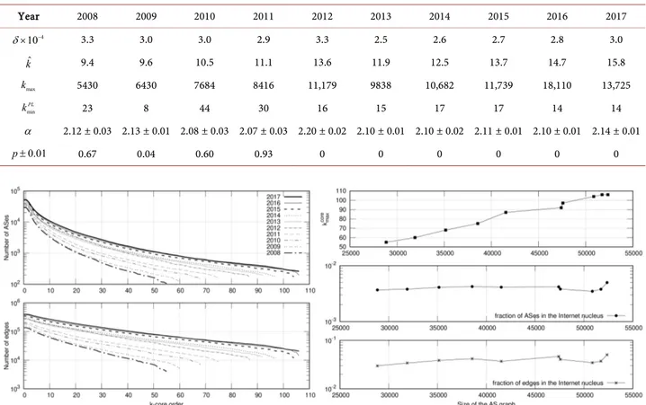
Figure 1 shows the node probability degree distributions and their complemen-tary cumulative functions (CCDF). For all data sets the peak of the degree dis-tribution is for k =2, a result already reported in [4] where it is claimed that it is due to the AS number assignment policies. While the edge density is around
4 3 10
δ ≈ × − during the decade 2008-2017, the general trend is a growth over time for both ˆk and kmax as shown in Table 3. This means that the Internet has become more connected preserving its sparse nature. All degree distribu-tions have a similar form. In order to verify the statistical plausibility of the power law model we perform a goodness of fit test based on the Kolmogo-rov-Smirnov statistic [20] which provides a p-value. The power law has statistic-al support if p >0.1. From Table 3 we see that even if the best-fit exponent is always around the value α ≈2.1 the power law can be considered a reliable
model only for the distributions of the years 2008, 2010 and 2011. Since for the majority of the largest data sets p ≤0.1, we could say that at the AS level the evolution of the Internet cannot be explained by models which predict a pure power law degree distribution.
4.2. K-Core Decomposition
The left plot of Figure 2 shows for each year of the decade 2008-2017 the distri-butions of ASes and edges in each k-core. We observe that in general for each
DOI: 10.4236/jcc.2019.78003 22 Journal of Computer and Communications Table 3.The table shows: the edge density δ, the average degree ˆk , the maximum degree kmax. The best fit power law cut off and exponent are k and minPL α. The condition p >0.1 indicates statistical plausibility of the power law model.
Year 2008 2009 2010 2011 2012 2013 2014 2015 2016 2017 4 10 δ× − 3.3 3.0 3.0 2.9 3.3 2.5 2.6 2.7 2.8 3.0 ˆk 9.4 9.6 10.5 11.1 13.6 11.9 12.5 13.7 14.7 15.8 max k 5430 6430 7684 8416 11,179 9838 10,682 11,739 18,110 13,725 min PL k 23 8 44 30 16 15 17 17 14 14 α 2.12 ± 0.03 2.13 ± 0.01 2.08 ± 0.03 2.07 ± 0.03 2.20 ± 0.02 2.10 ± 0.01 2.10 ± 0.02 2.11 ± 0.01 2.10 ± 0.01 2.14 ± 0.01 0.01 p ± 0.67 0.04 0.60 0.93 0 0 0 0 0 0
Figure 2. Left: number of ASes and edges in each k-core during the decade 2008-2017. Right: for each year of the decade 2008-2017 are shown, as a function of the size of the AS graph: the highest coreness kmaxcore (top); the percentage of ASes (middle) and edges (bottom) in the Internet nucleus.
k-core both the number of ASes and edges increase over time. The evolution of the Internet nucleus is shown in the right plot of Figure 2. The coreness of the nucleus increases over time (in 2016 and 2017 it has the same value). The frac-tion of ASes in the nucleus is quite stable over time although in absolute value Ɲn increases from 2008 to 2013, decreases in 2014 and 2015 and then increases again until 2017. We observe the same trend also for the number of edges in the nucleus as shown in Table 4.
On average the nucleus contains ~0.4% of all ASes and ~4% of all edges. Carmi
et al.[21] predicted the increase of kmaxcore and Ɲn as a power of N on the base of a numerical simulation assuming a scale-free growing model with the same para-meters of the real Internet. Instead, from the analysis of the Internet at the AS level during the period 2001-2006 Guo-Quing Zhang et al. [8] found no clear evidence of the exponential growth of kmaxcore and observed a stability of its value after 2003. They also found that the size of the nucleus exhibits large fluctuations over time.
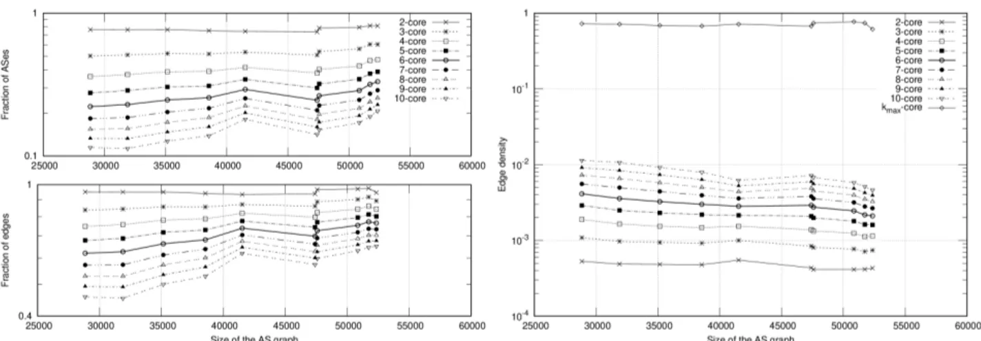
We now examine in the left plot of Figure 3 how the fraction of ASes and edges varies in the periphery of the Internet from the 2 to the 10-core. We start from the core of order 2 because in our case there are no isolated ASes.
DOI: 10.4236/jcc.2019.78003 23 Journal of Computer and Communications Figure 3.Left: fraction of ASes and edges in the periphery of the Internet from the 2 to the 10-core. Right: edge density δk as a function of the size of the AS graph for the k-cores and the Internet nucleus.
Table 4.Left: for each year in the decade 2008-2017 are shown the coreness kmaxcore of the Internet nucleus,and the number of ASes Ɲn and edges En it contains. Right: percentage variation in the number of ASes ∆Ɲkand edges ∆Ek in the core of order k obtained comparing 2008 and 2017 data. The last column reports the average edge density δk cal-culated over all the years 2008-2017.
Year kmaxcore Ɲn En K (core) ∆Ɲk (%) ∆Ek( )% δ k
2008 55 106 4040 2 4.82 −0.4 (42.1 ± 4.7) × 10−5 2009 60 121 5185 3 10.22 5.48 (79.8 ± 9.2) × 10−5 2010 68 144 7077 4 11.24 9.49 (13.0 ± 1.5) × 10−4 2011 75 163 8921 5 11.26 12.31 (19.2 ± 2.3) × 10−4 2012 87 171 10383 6 11.00 14.49 (26.5 ± 3.3) × 10−4 2013 92 198 13,132 7 10.56 16.13 (35.0 ± 4.6) × 10−4 2014 97 181 12,020 8 10.08 17.44 (44.6 ± 6.1) × 10−4 2015 104 177 12,008 9 9.57 19.3 (55.3 ± 7.8) × 10−4 2016 106 196 14,084 10 9.22 19.38 (6.8 ± 1.0) × 10−3 2017 106 261 20,838 max core k 0.13 2.05 (64.1 ± 6.8) × 10−2 Compared to the evolution of the nucleus it is evident that the periphery evolves with a different dynamics. In Table 4 we compare for each k-core the number of ASes and edges it contained in 2008 and 2017 and report the percentage varia-tion. Results clearly show that the nucleus is much more stable than the peri-phery. The connectivity of each core can be studied by looking at its edge density which is defined as
δ
k =2k k(
k−1)
. In the right plot of Figure 3 is shownk
δ as a function of N and in Table 4 is reported its average value. The edge
density increases with the coreness showing that the inner is the core the more it is connected. It is interesting to note that the edge density of the Internet nucleus is three order of magnitude higher than that of the most external 2-core. From a topological point of view this might imply the existence of an underlying
hie-DOI: 10.4236/jcc.2019.78003 24 Journal of Computer and Communications rarchical organization of the Internet with a small fraction of big ASes tightly connected among them and many regions composed of ASes with low or me-dium number of links. This structural property is investigated in more detail in the next section.
Tauro et al.[22] studied the topology of the Internet from the end of 1997 to the middle of 2000. They introduced the concept of importance of a node on the base of its degree and effective eccentricity defined as the minimum number of hops required to reach at least 90% of all other nodes. The most important nodes have high degree and low effective eccentricity. They found that the structure of the Internet is hierarchical with a highly connected core surrounded by layers of nodes of decreasing importance.
4.3. Clustering Coefficient
The clustering coefficient has been used to investigate the hierarchical organiza-tion of real networks. The hierarchy could be a consequence of the particular role of the nodes in the network. A stub AS does not carry traffic outside itself and is connected to a transit AS that, on the contrary, is designed for this pur-pose. The hierarchy of the Internet is rooted in its geographical organization in international, national backbones, regional and local areas. This is the skeleton of the Internet. International and national backbones are connected to regional networks which finally connect local areas to the Internet, implementing in such a way a best and less expensive strategy. It is reasonable to suppose that this hie-rarchical structure introduces correlations in the connectivity of the ASes. A. Vázquez et al.[2] showed that the hierarchical structure of the Internet is cap-tured by the scaling C k
( )
~k−γ and found γ =0.75. Ravasz and Barabasi [17] proposed a deterministic hierarchical model for which C k( )
~k−1 and using a stochastic version of the model showed that the hierarchical topology is again well described by the scaling C k( )
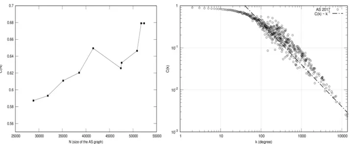
~k−γ even if the value of γ can be tuned by varying other network parameters.In the left plot of Figure 4 is shown the average clustering coefficient as a function of the size of the AS graph and in the fourth column of Table 5 is re-ported its value for all the years 2008-2017. Apart from the year 2013, C N
( )
weakly increases over time and the minimum and maximum values are ~0.59 and ~0.68 measured in 2008 and 2017, respectively. For the deterministic hie-rarchical model studied in [17], C is independent of N. The weak dependence ofC on N might indicate the presence of a hierarchical organization in the struc-ture of the Internet. To further investigate on this point, we study C k
( )
. The right plot of Figure 4 shows C k( )
for the AS graph only for the year 2017 be-cause for all other years the plots are almost overlapping. The best fit with the power law k−γ provides for all the years values of γ which differs only by ~0.1% obtaining, on average, γ =1.08 0.01± . In the same figure is also shown the slope of the function C k( )
~k−1 and even if it nicely follows the slope of the experimental points the goodness of fit test does not give any statistical supportDOI: 10.4236/jcc.2019.78003 25 Journal of Computer and Communications Figure 4.Left: average clustering coefficient as a function of the size of the AS graph during the decade 2008-2017. Right: average clustering coefficient as a function of the node’s degree for the AS graph of the year 2017. The solid line shows the slope
( )
~ 1C k k−
.
Table 5.For each year of the decade 2008-2017 are shown the average shortest path S, the diameter D and the average clustering coefficient C.
Year S ± 0.6 D C 2008 3.1 6 0.59 2009 3.0 7 0.59 2010 3.0 7 0.61 2011 3.0 6 0.62 2012 2.9 7 0.65 2013 3.0 6 0.63 2014 3.0 6 0.63 2015 3.0 6 0.65 2016 2.9 7 0.68 2017 2.9 7 0.68
to the scaling C k
( )
~k−γ. However, data show that C k( )
decreases with k especially for k >100. Low degree ASes have high neighbourhood connectivity and, on the contrary, neighbours of big hub ASes are slightly connected among them. This is consistent with a hierarchical organization in which big ASes are connected to many regions with high internal cohesiveness and composed of low or medium degree ASes, and these regions are poorly connected among them. Since the C k( )
plots of the AS graph snapshots overlap, to study the evolution of the clustering coefficient over years we compare the CCDF of( )
C k in Figure 5. For our convenience we consider in more detail three degree regions: high (k >1000), medium (100< ≤k 1000), low (k ≤100) and also plot them in the same figure. We observe that in the high degree region the CCDF
DOI: 10.4236/jcc.2019.78003 26 Journal of Computer and Communications Figure 5.CCDF of C k
( )
for the years 2008-2017 (top left). The figure shows in more detail the high (top right), medium (bottom left) and low (bottom right) degree regions. distributions are very intertwined indicating that during the decade 2008-2017 this region was rather static. In the medium degree region a clear separation emerges between the CCDF of the different years and for a given value of C k( )
the CCDF increases over time. The gap is even more pronounced in the peri-pheric low degree region. This result suggests that the evolution of the Internet from 2008 to 2017 was not uniform and the most significant changes mainly af-fected its middle and even more its periphery, and the neighborhood connectiv-ity in these regions increased over time.4.4. Shortest Path Length
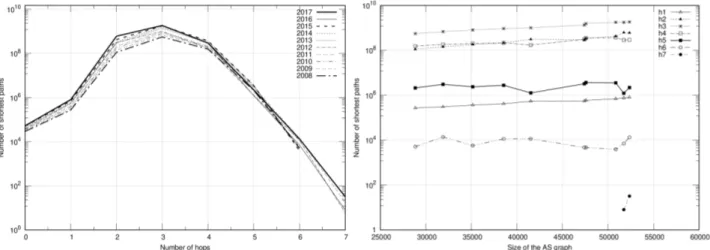
The left plot of Figure 6 shows the shortest path length distributions s h
( )
for all the years 2008-2017 and in Table 5 are reported the average values S and the diameter D. We observe that the overall trend is a slight decrease of S over time with an average of ~3.0. Zhao et al. [11] analyzed BGP data from the Route-Views Project [12] in the period 2001-2006 and observed a very weak decreasing of S. They measured a decreasing rate of ~2.5 × 10⁻⁴ and found S(
2001 3.4611)
= and S(
2006)
=3.3352. They noticed that simple power law and small worldmodels, which predict a growth of S with the size of the Internet, fail to explain the overall slight decrease of S over time and argued that this might be due to the fact that the Internet expands according to many factors not considered by sim-ple models like competitive and cooperative processes (like commercial rela-tionships), policy-driven strategy and other human choices. From the compari-son of our result with that of Zhao et al. there are indications the S has been slightly reduced during the period 2001-2017. This reinforces the fact that a pure power law model could not explain the evolution of the Internet because for
DOI: 10.4236/jcc.2019.78003 27 Journal of Computer and Communications Figure 6.Left: shortest path distributions s h
( )
for the AS graphs during the decade 2008-2017. Right: number of shortest paths of different lengths hn as a function of the size of the AS graph. Here hn indicates a shortest path whose length is n hops.2< <α 3 it predicts S~ ln lnN [23] [24]. The right plot of Figure 6 shows, for different lengths, the number of shortest paths over time. The 3-hops shortest paths are the most numerous, as expected, and their number increases over time.
4.5 Closeness Centrality
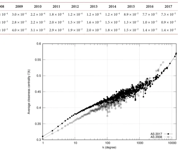
The closeness centrality Γ as a function of the node’s degree k is shown in
Figure 7 for the years 2008 and 2017. The plots of the other years have similar slope. Their curves lie in between of those plotted and are not shown in the fig-ure for better readability because they overlap in the region 100< <k 1000. We observe that Γ increases with the degree which means that big hub ASes are in the center of the Internet while low degree ASes are peripheric. We consider Γ in three regions: k ≤100, 100< ≤k 1000 and k >1000 corresponding re-spectively to low, medium and high degree and we find that within errors it is almost constant over the period 2008-2017 with average values of 0.392 ± 0.007, 0.434 ± 0.004 and 0.484 ± 0.004.
4.6. Betweenness Centrality
The average node betweenness centrality as a function of the degree k is shown in Figure 8 for the AS graphs of the years 2008 and 2017. As in the case of the closeness centrality, we do not plot the curves of the other years for readability reasons. However, for all the years the average node betweenness centrality in-creases with the degree which means that the higher is the degree of an AS the more is the number of shortest paths passing through it. There is evidence of an overall slight decrease of B kn
( )
during the evolution of the Internet from 2008to 2017. The overall average values of Bn calculated in 2008 and 2017 are ~7.1
× 10−5 and ~3.6 × 10⁻⁵ respectively. In Table 6 are reported the average values of
( )
n
B k calculated in the degree regions k ≤100, 100< ≤k 1000 and k >1000. In order to study Be we represent an edge as a point of the xy plane whose
DOI: 10.4236/jcc.2019.78003 28 Journal of Computer and Communications Table 6.Average node betweenness centrality Bn in the degree regions k ≤100, 100< ≤k 1000 and k >1000.
( ) n B k 2008 2009 2010 2011 2012 2013 2014 2015 2016 2017 100 k ≤ 3.3 × 10⁻⁴ 3.0 × 10⁻⁴ 2.2 × 10⁻⁴ 1.8 × 10⁻⁴ 1.2 × 10⁻⁴ 1.2 × 10⁻⁴ 1.2 × 10⁻⁴ 8.9 × 10⁻⁵ 7.7 × 10⁻⁵ 7.3 × 10⁻⁵ 100< ≤k 1000 3.0 × 10⁻³ 2.8 × 10⁻³ 2.2 × 10⁻³ 2.0 × 10⁻³ 1.5 × 10⁻³ 1.6 × 10⁻³ 1.5 × 10⁻³ 1.3 × 10⁻³ 1.0 × 10⁻³ 0.9 × 10⁻³ 1000 k > 4.5 × 10⁻² 4.0 × 10⁻² 3.1 × 10⁻² 2.9 × 10⁻² 1.9 × 10⁻² 2.0 × 10⁻² 1.8 × 10⁻² 1.5 × 10⁻² 1.4 × 10⁻² 1.4 × 10⁻²
Figure 7.Average closeness centrality Γ
( )
k as a function of the degree k for the AS graphs of the years 2008 and 2017.Figure 8.Average node betweenness centrality B kn
( )
as a function of the degree k for the AS graphs of the years 2008 and 2017.DOI: 10.4236/jcc.2019.78003 29 Journal of Computer and Communications Figure 9.Average edge betweenness centrality Be for the AS graphs of the years 2008-2017. Left: color mapped 3D plots of Be. To each edge is associated with a point of the xy plane whose coordinates
(
k k x, y)
are the degree of the nodes it connects. Right: colored contour maps of the figures on the left.shown, for each year of the decade 2008-2017, the colored 3D map of the average
e
B . The highest Be is associated to edges which have at least a high degree
(k >1000) AS as a terminal. Edges connecting low or medium degree ASes have lower Be. This is what one would expect considering that high degree ASes are
the backbone of the Internet and the most part of the shortest routes should cross them. We also observe a slight decrease of Be over time. The overall
av-erage Be was ~2.2 × 10⁻⁵ in 2008 and ~0.7 × 10⁻⁵ in 2017, indicating that
some-how the Internet has become less congested although it has expanded. By look-ing at the colored contour maps shown on the right side of Figure 9 we infer that during its evolution the lowering of Be affected first the part of the
Inter-net containing low and medium degree ASes (k <1000) and subsequently the backbone. The overall average values of Bn and Be were measured also in [4]
for three sources of data. Authors found that for the AS graph of the Internet constructed from the CAIDA Skitter [25] repository with data collected in March 2004 Bn and Be were ~11.0 × 10⁻⁵ and ~5.4 × 10⁻⁵. This is a further
confirmation that during the evolution of the Internet the traffic load somehow decreases. This may be due to the adoption of more efficient routing policies and to infrastructural upgrades with more advanced network devices.
5. Conclusion
We studied the evolution of the Internet at the AS level during the decade 2008-2017. For each year of the decade we considered a snapshot of the AS un-directed graph and analyzed how a wide range of metrics related to structure, connectivity and centrality varies over time. During the decade 2008-2017 the Internet almost doubled its size and became more connected. The Internet is a scale-free network because it contains both very high and low degree ASes. For all the years 2008-2017 the best fit of the degree distributions with a power law
( )
~DOI: 10.4236/jcc.2019.78003 30 Journal of Computer and Communications around α ≅2.1. However, the statistical analysis shows that a pure power law
model fails to explain the scale-free properties. The study of the k-core decom-position shows that Internet has a small internal nucleus composed of high de-gree ASes much more stable and connected than external cores. We investigated the hierarchical organization of the Internet by studying the average clustering coefficient C. We found that there are indications of an overall hierarchical or-ganization of the Internet where a small fraction of big ASes are connected to many regions with high internal cohesiveness containing low and medium de-gree ASes and these regions are slightly connected among them. The average shortest path length S of the Internet slightly decreased during the decade 2008-2017 form ~3.1 to ~2.9 measured in 2008 and 2016-2017 respectively. Re-gardless of the analyzed year, the closeness centrality Γ of an AS increases with its degree. Hence, big ASes are in the center of the Internet and low degree ASes are in the periphery. It is reasonable to assume that the traffic load of an AS or car-ried by an edge is proportional to the number of shortest paths passing through the AS and containing the edge. These measurements can be quantified by the av-erage node and edge betweenness centrality Bn and Be. There is evidence of
an overall slight decrease of both Bn and Be during the decade 2008-2017,
suggesting that during its evolution the Internet became less congested.
Acknowledgements
The computing resources and the related technical support used for this work have been provided by CRESCO/ENEAGR\-ID High Performance Computing infrastructure and its staff [26]. CRESCO/ENEAGRID High Performance Com-puting infrastructure is funded by ENEA, the Italian National Agency for New Technologies, Energy and Sustainable Economic Development and by Italian and European research programmes, see https://www.eneagrid.enea.it for in-formation.
Conflicts of Interest
The authors declare no conflicts of interest regarding the publication of this pa-per.
References
[1] Rekhter, Y., Li, T. and Hares, S. (2006) A Border Gateway Protocol 4. RFC 4271. Internet Engineering Task Force.
[2] Vázquez, A., Pastor-Satorras, R. and Vespignani, A. (2002) Internet Topology at the Router and Autonomous System Level.
[3] Zhang, B., Liu, R., Massey, D. and Zhang, L. (2005) Collecting the Internet AS-Level Topology. ACM SIGCOMM Computer Communication Review, 35, 53-61.
https://doi.org/10.1145/1052812.1052825
[4] Mahadevan, P., Krioukov, D., Fomenkov, M., Dimitropoulos, X., Claffy, K.C. and Vahdat, A. (2006) The Internet AS-Level Topology: Three Data Sources and One DefinitiveMetric. ACM SIGCOMM Computer Communication Review, 36, 17-26.
DOI: 10.4236/jcc.2019.78003 31 Journal of Computer and Communications https://doi.org/10.1145/1111322.1111328
[5] Magoni, D. and Pansiot, J.J. (2001) Analysis of the Autonomous System Network Topology. ACM SIGCOMM Computer Communication Review, 31, 26-37.
https://doi.org/10.1145/505659.505663
[6] Edwards, B., Hofmeyr, S., Stelle, G. and Forrest, S. (2012) Internet Topology over Time.
[7] Dhamdhere, A. and Dovrolis, C. (2008) Ten Years in the Evolution of the Internet Ecosystem. Proceedings of the 8th ACM SIGCOMM Conference on Internet Mea-surement, Vouliagmeni, 20-22 October 2008, 183-196.
https://doi.org/10.1145/1452520.1452543
[8] Zhang, G.-Q., Zhang, G.-Q., Yang, Q.-F., Cheng, S.-Q. and Zhou, T. (2008) Evolu-tion of the Internet and Its Cores. New Journal of Physics, 10, Article ID: 123027.
https://doi.org/10.1088/1367-2630/10/12/123027 [9] CAIDA.
http://www.caida.org/data/active/ipv4_routed_topology_aslinks_dataset.xml [10] CAIDA. Archipelago Measurement Infrastructure.
http://www.caida.org/projects/ark
[11] Zhao, J. (2008) Does the Average Path Length Grow in the Internet? Information Networking. Towards Ubiquitous Networking and Services. Springer, Berlin Hei-delberg.https://doi.org/10.1007/978-3-540-89524-4_19
[12] http://www.routeviews.org
[13] Faloutsos, M., Faloutsos, P. and Faloutsos, C. (1999) On Power-Law Relationships of the Internet Topology. ACM SIGCOMM Computer Communication Review, 29, 251-262.https://doi.org/10.1145/316194.316229
[14] Chen, Q., Chang, H., Govindan, R., Jamin, S., Shenker, S. and Willinger, W. (2002) The Origin of Power-Laws in Internet Topologies Revisited. 21st Annual Joint Conference of the IEEE Computer and Communications Societies, New York, 23-27 June 2002, 608-617.
[15] Barabasi, A. and Albert, R. (1999) Emergence of Scaling in Random Networks. Science, 286, 509-512.https://doi.org/10.1126/science.286.5439.509
[16] Vázquez, A., Pastor-Satorras, R. and Vespignani, A. (2002) Large-Scale Topological and Dynamical Properties of the Internet. Physical Review E, 65, Article ID: 066130.
https://doi.org/10.1103/PhysRevE.65.066130
[17] Ravasz, E. and Barabasi, A. (2003) Hierarchical Organization in Complex Networks. Physical Review E, 67, Article ID: 026112.
https://doi.org/10.1103/PhysRevE.67.026112
[18] Holme, P. and Kim, B.J. (2002) Vertex Overload Breakdown in Evolving Networks. Physical Review E, 65, Article ID: 066109.
https://doi.org/10.1103/PhysRevE.65.066109
[19] Goh, K.I., Kahng, B. and Kim, D. (2001) Universal Behavior of Load Distribution in Scale-Free Networks. Physical Review Letters, 87, Article ID: 278701.
https://doi.org/10.1103/PhysRevLett.87.278701
[20] Clauset, A., Shalizzi, C.R. and Newman, M.E.J. (2009) Power Law Distributions in Empirical Data. SIAM Review, 51, 661-703.https://doi.org/10.1137/070710111 [21] Carmi, S., Havlin, S., Kirkpatrick, S., Shavitt, Y. and Shir, E. (2007) A Model of
In-ternet Topology Using k-Shell Decomposition. Proceedings of the National Acade-my of Sciences, 104, 11150-11154.https://doi.org/10.1073/pnas.0701175104
DOI: 10.4236/jcc.2019.78003 32 Journal of Computer and Communications Model for the Internet Topology. IEEE Global Telecommunications Conference, San Antonio, 25-29 November 2001, Vol. 3, 1667-1671.
[23] Cohen, R. and Halvin, S. (2003) Scale-Free Networks Are Ultrasmall. Physical Re-view Letters, 90, Article ID: 058701.https://doi.org/10.1103/PhysRevLett.90.058701 [24] Bollobás, B. and Riordan, O. (2004) The Diameter of a Scale-Free Random Graph.
Combinatorica, 24, 5-34.https://doi.org/10.1007/s00493-004-0002-2 [25] Claffy, K., Monk, T. and McRobb, D. (1999) Internet Tomography. Nature.
[26] Iannone, F., et al. (2019) CRESCO ENEA HPC Clusters: A Working Example of a Multifabric GPFS Spectrum Scale Layout. Proceedings of the 2019 International Conference on High Performance Computing & Simulation, Dublin, 15-19 July 2019.