Dynamics of vehicles with controlled limited-slip differential

(1)

Scuola di Dottorato in Ingegneria “Leonardo da Vinci”

Corso di Dottorato di Ricerca in

Veicoli Terrestri e Sistemi di Trasporto

Tesi di Dottorato di Ricerca

Dynamics of vehicles with controlled

limited-slip differential

Candidato

Ing. Giordano Greco

Tutori

Prof. Ing. Antonio Bicchi Prof. Ing. Massimo Guiggiani

(2)

(3)

This Ph.D. thesis is aimed at analyzing vehicle dynamics in presence of an electronically controlled limited-slip differential and at developing advanced control strategies for the limited-slip differential of sports cars, in order to improve performance, stability and safety. A critical review of the concept of understeer-oversteer for vehicles with locked differential is first presented. The steady-state directional behaviour of rear-wheel drive vehicles fitted with locked differential is theoretically analyzed. Furthermore, the problem of describing the understeer-oversteer behaviour of a general vehicle is ad-dressed taking a fresh perspective, since the new concept of handling surface and a new definition of understeer gradient are presented, this latter being the gradient of the handling surface. The problem of controlling vehicle dynamics by means of electronically controlled limited-slip differentials is then approached. The main handling control problems for sports cars fitted with controlled limited-slip differential are analyzed in detail. An advanced control strategy, developed for the rear electronically controlled limited-slip differential of F1 race cars, is also described.

(4)

(5)

To my parents Zanetta and Gaetano and my grandmother Adriana At the end of these three years of Ph.D. studies, I wish to thank first my par-ents Zanetta and Gaetano and my grandmother Adriana, for all the things they have done for me and for their neverending support and encouragement. I deeply wish to thank Prof. Massimo Guiggiani and Prof. Antonio Bicchi, for all the interesting things they have taught to me and for all the experiences and opportunities I had while working with them.

I wish to thank everybody has studied and worked with me during these three years: Francesca Di Puccio, Francesco Frendo, Simona Celi, Simo-netta Boria, Marco Gabiccini, Alessio Artoni, Antonio Sponziello, Gabriele Melani, Francesco Bartaloni, Nicola Sgambelluri, Daniele Fontanelli, Adri-ano Fagiolini, Riccardo Schiavi, Antonio Danesi.

I also wish to acknowledge Marco Fainello, Ignazio Lunetta, Gabriele Pieraccini, Maurizio Bocchi and Carlo Miano for the opportunity they gave me to work in contact with Ferrari race team.

Many thanks to my close friends Lucia Pallottino and Giovanni Tonietti, for the beautiful experiences we had together and for all the things they have taught to me, not only from a scientific and technical point of view.

Many thanks to Tiziana Spadafina, for her close friendship and neverend-ing encouragement durneverend-ing these years of studies.

(6)

(7)

Sintesi in Italiano – Summary in Italian 11

Introduction to the thesis 15

1 Directional behaviour of vehicles with locked differential 19

1.1 Introduction . . . 19

1.2 Classical results . . . 22

1.2.1 The single track vehicle model . . . 22

1.2.2 The handling diagram for the single track vehicle model 25 1.3 Model of a vehicle with locked differential . . . 27

1.3.1 Equilibrium equations . . . 29

1.3.2 Congruence equations: tyre theoretical slips . . . 30

1.3.3 Constitutive equations: tyre model . . . 32

1.3.4 Vertical load on each tyre . . . 34

1.4 Vehicle model with linear tyre behaviour . . . 36

1.4.1 Forces acting on the axles and yaw moment . . . 37

1.4.2 Steady-state cornering behaviour . . . 39

1.5 Vehicle model with non linear tyre behaviour . . . 47

1.6 Conclusions . . . 53

2 The handling surface theory 55 2.1 Introduction . . . 55

2.2 The handling surface H . . . . 57

2.3 A more general definition of the understeer gradient . . . 61

2.4 Geometrical interpretation of the understeer gradient Km . . 63

2.5 Many handling curves from the same handling surface . . . . 64

(8)

2.7 How to measure w . . . 67

2.8 The handling surface for the single track model . . . 68

3 Two handling surfaces 71 3.1 Introduction . . . 71

3.2 The two handling surfaces A and Y . . . 72

3.3 Definition of the understeer gradient . . . 76

3.4 Geometrical interpretation of the understeer gradient Km . . 78

3.5 The particular case of the single track vehicle model . . . 82

4 Vehicle model with controlled differential 85 4.1 Introduction . . . 85

4.2 Vehicle model . . . 86

4.2.1 Equilibrium equations . . . 87

4.2.2 Congruence equations: tyre theoretical slips . . . 89

4.2.3 Constitutive equations: tyre model . . . 89

4.2.4 Vertical load on each tyre . . . 90

4.2.5 Equilibrium equations of the front wheels . . . 92

4.3 Model of the transmission system . . . 92

4.3.1 Equilibrium equations of the rear wheels . . . 95

4.3.2 Equilibrium equation of the differential pinion . . . 95

4.3.3 Equilibrium equation of the differential case . . . 96

4.3.4 Equations of motion of the rear axle . . . 96

4.4 Different models for locked and slipping conditions . . . 97

4.5 State-space form of the equations of motion . . . 101

4.6 Results from simulations . . . 102

5 Control strategies for semi-active differentials of sports cars109 5.1 Introduction . . . 109

5.2 Handling control problems for sports cars . . . 110

5.2.1 Braking conditions during corners . . . 111

5.2.2 Traction conditions during corners . . . 119

5.3 Control strategy for the differential of a F1 race car . . . 125

5.3.1 Typical handling conditions for a F1 race car . . . 126

(9)

5.3.3 Estimate of the differential torque in locked conditions 128 5.3.4 Control logic in braking and end-of-braking conditions 129 5.4 Conclusions . . . 133

6 Conclusions and final remarks 135

List of main symbols 137

(10)

(11)

Summary in Italian

Dinamica dei veicoli con differenziale a slittamento

controllato

Questa tesi di Dottorato di Ricerca ha due obiettivi principali. Il primo è lo studio analitico e sperimentale del comportamento direzionale dei veicoli dotati di differenziale a slittamento controllato, detto anche differenziale semi attivo. Il secondo è lo sviluppo di strategie di controllo avanzate per il differenziale a slittamento controllato di vetture sportive, per migliorarne il comportamento direzionale e la stabilità di marcia in condizioni di guida al limite.

All’opposto dei differenziali ordinari, i differenziali autobloccanti sono in grado di ripartire in modo asimmetrico la coppia del motore tra le ruote motrici. Oltre a ci`o, i differenziali a slittamento controllato sono dotati di servo meccanismi, i quali sono in grado di modificare il rapporto tra le coppie trasmesse alle ruote motrici secondo una logica di controllo che, istante per istante, tiene conto delle condizioni operative del veicolo.

I differenziali autobloccanti e i differenziali a slittamento controllato in-fluenzano fortemente la dinamica dei veicoli. Essi hanno effetti importanti sul carattere sovra-sottosterzante e sulle capacità di trazione e di frenatura. La dinamica del veicolo, infatti, è prevalentemente influenzata dalle forze che la strada trasmette ai pneumatici. D’altra parte, le forze longitudi-nali che agiscono sui pneumatici dipendono dalle condizioni di aderenza del contatto ruota - terreno e dall’entità delle coppie che i freni e il differen-ziale applicano alle ruote. Di conseguenza, modificando l’entità delle coppie

(12)

trasmesse dai freni e dal differenziale, `e possibile influenzare la dinamica dei veicoli.

Per tutte queste ragioni, l’impiego di differenziali a slittamento control-lato su vetture sportive e da competizione può portare ad un miglioramento delle prestazioni in curva. Controllando opportunamente il trasferimento di coppia tra le ruote motrici, questi differenziali possono determinare un miglioramento delle capacità di trazione e di frenatura, della stabilità e della controllabilità della vettura. I differenziali a slittamento controllato vengono anche impiegati sulle vetture da F1. Lo sviluppo di strategie di controllo per la gestione dei differenziali semi attivi rappresenta un obiettivo di primaria importanza per tutte le scuderie in gara.

Gli studi classici di dinamica del veicolo si basano principalmente su mo-delli di veicolo molto semplici, come il ben noto modello monotraccia. Questi modelli, sebbene possano essere considerati rappresentativi per veicoli dotati di differenziale ordinario, sono del tutto inadeguati per lo studio della dinam-ica del veicolo in presenza di un differenziale autobloccante o a slittamento controllato. In questi casi, infatti, è necessario impiegare modelli matematici di veicolo ben più sofisticati. Inoltre, è necessario sviluppare nuove teorie di riferimento, diverse da quella classica, che aiutino nell’interpretazione dei risultati sperimentali e di quelli ottenuti da simulazione.

In particolare, il classico concetto di sovra-sottosterzo, che si basa sul diagramma di maneggevolezza, e quindi sulla teoria del modello monotrac-cia, deve essere rivisitato criticamente e riformulato per veicoli dotati di differenziale autobloccante o a slittamento controllato.

Questa tesi raccoglie i principali risultati dell’attività di studio portata avanti nei tre anni di Dottorato di Ricerca. Alcuni di questi risultati sono stati presentati in due articoli. Il primo è stato pubblicato sulla rivista internazionale Vehicle System Dynamics, mentre il secondo è stato recente-mente accettato per la pubblicazione in questa stessa rivista. La prima parte della tesi, quindi, presenta i contenuti di questi articoli, assieme a successivi sviluppi ed elaborazioni.

Entrambi gli articoli riportano i risultati di una rivisitazione critica del concetto di sovra-sottosterzo per veicoli dotati di differenziale bloccato. Il primo articolo ([11]) presenta un’analisi teorica del comportamento direzio-nale a regime dei veicoli a trazione posteriore dotati di differenziale bloccato. Il secondo articolo ([12]) presenta una generalizzazione della teoria esposta nel primo articolo. Infatti, in esso viene introdotto uno strumento innovativo

(13)

per la caratterizzazione completa del comportamento direzionale a regime di un qualsiasi veicolo, la superficie di maneggevolezza, che va a rimpiazzare il classico diagramma di maneggevolezza. Inoltre, l’articolo propone una nuova definizione di gradiente di sottosterzo che, a differenza di quello clas-sico, `e un vettore e non uno scalare. I nuovi concetti introdotti rappresentano una generalizzazione di quelli classici, che si basano sulla teoria del modello monotraccia.

Entrambi gli articoli prendono in esame il caso di un veicolo dotato di differenziale bloccato. Sicuramente, questa è una condizione di funziona-mento molto particolare per un differenziale autobloccante o a slittafunziona-mento controllato. È comunque una condizione molto significativa, poiché in curva il differenziale di una vettura da F1 viene tenuto bloccato per buona parte del tempo.

L’argomento del controllo della dinamica del veicolo per mezzo di dif-ferenziali a slittamento controllato `e affrontato nella seconda parte della tesi.

Prima di tutto, viene descritto un modello matematico di veicolo, in grado di rappresentare il comportamento di una vettura a trazione posteriore dotata di differenziale a slittamento controllato sia in condizioni di moto stazionario che in condizioni di transitorio dinamico, quali manovre di tiro, di rilascio e di frenata.

Successivamente, vengono analizzate in dettaglio le principali influenze di un differenziale a slittamento controllato sul comportamento dinamico di vetture sportive. In particolare, vengono considerati gli effetti sulle capacit`a di trazione e di frenatura, sul comportamento sovra-sottosterzante e sulla stabilit`a di marcia. L’analisi viene corredata con la descrizione dei risultati di simulazioni di manovre dinamiche, considerate significative.

Infine, vengono descritti i risultati di un’attività di ricerca portata avanti in collaborazione con Ferrari S.p.a., con l’obiettivo di definire una strategia di controllo innovativa per il differenziale a slittamento controllato di vetture da F1. Data la natura strettamente riservata della ricerca e l’importanza strategica dei suoi risultati, la logica di controllo sviluppata viene qui de-scritta solamente in modo qualitativo. Preme, però, sottolineare che questa strategia di controllo è stata implementata in vettura e che sono state effet-tuate prove su pista, ottenendo risultati soddisfacenti.

(14)

(15)

This Ph.D. thesis has two main goals. The first one is the analytical and experimental study of the cornering behaviour of vehicles fitted with an electronically controlled limited-slip differential, also called semi-active dif-ferential. The second one is the development of advanced control strategies, to be applied to the electronically controlled limited-slip differential of sports cars, in order to optimize both handling and stability under severe driving conditions.

Unlike the open or free differential, limited-slip differentials are able to split the torque from the engine to the driving wheels in an asymmetric way. Furthermore, electronically controlled limited-slip differentials are fitted with servo mechanisms, which are able to modify the ratio between the torques delivered to the driving wheels, according to a control logic and depending on the actual working condition of the vehicle.

Limited-slip differentials have major effects on vehicle dynamics, since they play an important role in determining the understeer-oversteer be-haviour. Moreover, they affect traction and braking capabilities, possibly leading to substantial improvements.

The dynamic behaviour of vehicles is in fact mainly influenced by the forces which the road applies to the tyres. On the other hand, longitudinal tyre forces depend on adherence conditions and on torques which the brake system and the differential deliver to the tyres. Therefore, by changing the magnitude of the torques from brakes and from the differential, it is possible to affect vehicle dynamics.

For these reasons, electronically controlled limited-slip differentials repre-sent devices which can be usefully adopted to improve performance of sports cars during corners. By suitably controlling the torque transfer between the driving wheels, such differentials can enhance traction and braking capa-bilities, stability and controllability. Electronically controlled limited-slip

(16)

differentials are also commonly employed in F1 race cars. The development of control strategies for their management is a goal of great importance for all teams involved in competitions.

Vehicle dynamics is classically analysed by means of very simple vehicle models, such as the well known single track model. Such models can properly represent the dynamic behaviour of vehicles fitted with open differential, but they are completely inadequate for vehicles fitted with a locked or limited-slip differential. In these cases, more sophisticated vehicle models must be employed. Furthermore, a new reference theory, different from the classical one, should be developed in order to deeply understand both experimental and simulated results.

In particular, the classical concept of understeer-oversteer, which is based on the handling diagram, and hence on the single track model theory, should be critically reviewed and reformulated for vehicles with non-free differential. Moving from these considerations, this thesis collects the main results of the study carried out during the three years of the Ph.D. research activity. Some of these results have been presented in two papers. The first one has been published in the journal Vehicle System Dynamics, while the second one has been accepted for publication in the same journal. Therefore, the first part of the thesis presents the contents of these papers, along with subsequent revisions and further developments.

In both papers, results of a critical review of the concept of understeer-oversteer for vehicles with locked differential are discussed. The first paper ([11]) presents a theoretical analysis of the steady-state cornering behaviour of rear-wheel drive vehicles fitted with locked differential. The second paper ([12]) represents the generalization of the theory presented in the first paper. It introduces a quite innovative and useful tool for the complete character-ization of the steady-state directional behaviour of any kind of vehicle, the handling surface, which should replace the well known handling diagram. It also proposes a new definition of understeer gradient, which is a vector, unlike the classical understeer gradient, which is a scalar. The new concepts here introduced generalize the classical ones, which are based on the theory of the single track model.

Both papers refer specifically to vehicles fitted with locked differential, which represents a quite particular operation mode of a limited-slip differ-ential. However, this is a significant condition, since it frequently occurs for race cars during corners.

(17)

The problem concerning the active control of vehicle dynamics by means of limited-slip differentials is approached in the second part of the thesis.

A vehicle model is first introduced, which is able to represent the dy-namic behaviour of a rear-wheel drive vehicle fitted with an electronically controlled limited-slip differential under both steady-state and transient con-ditions (power-on, power-off and braking manoeuvres).

The most important effects of electronically controlled limited-slip differ-entials on the dynamic behaviour of sports cars are then analyzed in detail. Traction and braking performance, understeer-oversteer characteristics and stability aspects are investigated also by means of simulations.

Finally, results of a research activity carried out in cooperation with Ferrari S.p.a. are presented. The aim of this activity was the development of an advanced control strategy, to be applied to the rear electronically controlled limited-slip differential of a F1 race car, in order to optimize handling performance. Owing to their strictly confidential nature and their strategic importance for Ferrari race team, results are here discussed only in a qualitative way.

The structure of the thesis is organized as follows.

In Chapter 1, after having summarized the main aspects of the classical theory of the single track vehicle model, the analysis of the steady-state di-rectional behaviour of rear-wheel drive vehicles fitted with locked differential is presented.

Chapter 2 describes the theory of the handling surface.

Chapter 3 presents the theory of the two handling surfaces. This analysis represents a further development of that described in Chapter 2.

Chapter 4 introduces the vehicle model with electronically controlled limited-slip differential, which has been developed for the analysis of vehicle dynamics under both steady-state and transient conditions.

Chapter 5 presents the analysis of the main handling control problems for rear-wheel drive sports cars fitted with electronically controlled limited-slip differential and describes the control strategy developed for the limited-slip differential of Ferrari F1 race cars.

(18)

(19)

Directional behaviour of

vehicles with locked

differential

1.1 Introduction

The single track model theory is typically employed for the analysis of vehi-cle dynamics. Even though such a theory is based on a very simple vehivehi-cle model, it has been largely used to understand and foresee the dynamic be-haviour of real vehicles ([34, 8, 15, 30, 16]).

In the classical single track model, a rear-wheel drive vehicle fitted with an open differential and moving at constant longitudinal speed is considered. Due to the open differential, traction forces acting on the rear tyres are always equal. Moreover, owing to some strong assumptions, the slip angles of the tyres belonging to the same axle are assumed equal and longitudinal slips are neglected. According to these hypotheses, a relationship between the whole side force and the slip angle of each axle can be found, leading to a model fitted with only two equivalent tyres.

One of the most relevant results of this approach is that a single handling curve, the so-called handling diagram, only depending upon the constructive parameters, describes completely the steady-state cornering behaviour of the vehicle. The slope of such a curve represents the understeer gradient, which is a measure of the degree of understeer-oversteer to be associated to each level of lateral acceleration, and therefore to each steady-state cornering

(20)

condition. Moreover, this diagram can supply some relevant information about the stability of the equilibrium states, showing the regions of stable and unstable motion.

The main properties of the handling diagram were first discussed in [34]. The handling diagram can be easily obtained by means of experimental ground tests and is often employed for the experimental assessment of vehicle dynamics ([20, 15]).

However it is, perhaps too often, not sufficiently appreciated that some of its properties heavily rely on the hypotheses behind the classical single track model. Indeed, it will be shown that, although this model can be pro-perly used to characterize the cornering behaviour of vehicles endowed with open differential, it becomes completely inadequate for vehicles fitted with locked differential. In fact, when a vehicle with locked differential negotiates a corner, the driving wheels are forced to rotate at the same angular velocity and longitudinal slips become not negligible, considerably influencing vehicle dynamics. In order to analyse these effects, it is necessary to formulate a four-wheel model and take into account both the lateral and longitudinal slips of each tyre. Moreover, for a vehicle fitted with a locked differential, during a corner tractive forces acting on the driving wheels may be differ-ent. That provides a yaw moment which strongly affects the directional behaviour.

The effect of locked differentials and limited-slip differentials, both con-ventional self-locking and actively controlled, on vehicle dynamics has been largely described by many authors ([1, 17, 27, 26, 25, 29, 33, 18]). The influ-ence of the distribution of longitudinal tyre forces, caused by such devices, on traction and braking capabilities and directional behaviour has been in-vestigated by means of both numerical simulations and experimental ground tests.

Moreover, Abe described in [1], by means of an approximate analytical method, the effect of locked differentials on the cornering behaviour in ac-celeration and in braking. Results were compared with those obtained by means of numerical simulations, showing a good agreement.

Nowadays, electronically-controlled limited-slip differentials, as well as steering and traction control systems, may lead to substantial improvements of performance, stability and manoeuvrability during corners ([26, 25, 40, 33, 37, 2, 18, 13, 31, 32]).

(21)

ve-hicle dynamics, the development of a reference theory seems to be necessary. Such a theory, which appears not to have been sufficiently developed yet, should have the same role the classical single track model theory has with respect to vehicles fitted with open differential; that means it should be the analytical basis for the comprehension of vehicle dynamics when a locked or limited-slip differential is employed. According to a well-established tradi-tion in vehicle dynamics studies, it seems profitable to continue to charac-terize the cornering behaviour of vehicles by means of some typical tools and concepts, such as the handling diagram and the understeer gradient, which are largely used in the single track model theory, even though, as it will be shown, a critical review of both of them is necessary.

In order to have a clear and general picture of the problems involved, it may be convenient to develop simple vehicle models, having few degrees of freedom, but being able to represent the most important characteristics of the motion all the same. In this study we deal with vehicles fitted with a locked differential, which represents a very particular operation mode of a limited-slip differential, but is also the easiest condition to deal with. How-ever, this is a significant condition, since it frequently occurs for race cars during corners.

An approximate theoretical analysis of the effect of a non-free differential on vehicle dynamics is given in [8]; however, in that work the effects of combined slip operation of tyres are not considered and the vehicle steady-state behaviour is not investigated in detail. An experimental investigation of the dynamic behaviour of a rear-wheel drive vehicle with locked differential was given in [10], while preliminary theoretical models for analysing the dynamics of such a vehicle were presented in [3, 4]. The effects on the handling diagram of the yaw moment, arising from the difference between the rear longitudinal forces, were investigated in those papers; in addition, the handling diagram was shown to depend on the motion parameters, and not only on the vehicle features.

In the present study a general theoretical analysis of the steady-state cor-nering behaviour of rear-wheel drive vehicles fitted with locked differential is proposed. A detailed description of tyre kinematics under combined slip conditions is first developed. Two vehicle models are then defined, having linear and non linear tyre properties respectively. Such models are deliber-ately simple. However, they allow to catch the basic aspects of the dynamics of vehicles fitted with locked differential and to perform a theoretical and

(22)

systematic approach to the topic.

The steady-state cornering behaviour is then investigated and the han-dling diagrams are obtained in several manoeuvres. For the model with linear tyres, analytical expressions of the understeer gradient are also obtained. As opposite to the classical definition, the handling diagram is shown not to be unique.

Results clearly show the inadequacy of the classical single track model to characterize the cornering behaviour of vehicles with locked differential. They also suggest a more critical and careful use of some typical tools and concepts, such as the handling diagram or the understeer gradient. More-over, the approach here proposed may represent the basis of a new reference theory, to be added to the classical single track model theory for the analysis of vehicle dynamics when a locked differential is employed.

The analysis, which is presented in this chapter, has been recently pub-lished in [11].

1.2 Classical results

The classical single track vehicle model is the most popular mathematical model for the analysis of the directional behaviour of vehicles. Its properties have been largely described in the scientific literature ([34, 8, 15, 30, 16]). However, it seems convenient to summarize briefly the main characteristics of such model, in order to understand the results of the studies presented in this thesis.

1.2.1 The single track vehicle model

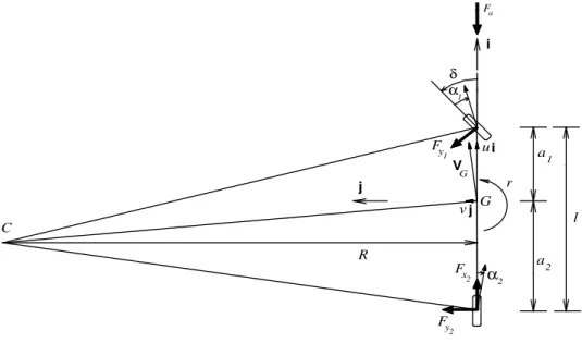
The single track vehicle model refers to a rear-wheel drive vehicle fitted with an open differential. As shown in Fig. 1.1, the vehicle model is represented as a rigid body fitted with only two equivalent tyres, which simulate the behaviour of the front and rear axles. The motion of the vehicle is plane and parallel to the road, which is assumed to be horizontal and perfectly even. It is common practice to define a reference frame (x, y, z; G) attached to the vehicle, whose origin coincides with the centre of mass G and whose versors are (i, j, k). Axes i and j are parallel to the road. The direction of axis i coincides with the forward direction of the vehicle, while axis j is orthogonal to that direction. Axis k is orthogonal to the road and points upwards.

(23)

C R v j G 2 α r α u V G δ i 1 2 a l 1 a F_y 2 2 x F F_y 1 i j a F

Figure 1.1: The classical single track vehicle model.

The model has three state variables: the longitudinal speed u, the lateral speed v and the yaw rate r. The speeds u and v are the longitudinal and lateral components of the absolute speed VG of the centre of mass G

V_G= u i + v j. (1.1)

Under normal driving conditions the following relation holds: u À |v|. The yaw rate r is the only component of the angular velocity Ω of the vehicle: Ω = r k.

The slip angle β of the vehicle is defined as β = arctan³ v

u ´

' v

u. (1.2)

In Fig. 1.1, a1 and a2 are the longitudinal distances between the centre

of mass G and each axle, l = a1+ a2 is the wheelbase, δ is the front steer

(24)

The front and rear slip angles are defined as α1= δ −v + ra_u 1,

α2= −v − ra_u 2.

(1.3) The variable R = u/r represents the distance between the instantaneous centre of rotation C of the vehicle and the longitudinal vehicle axis. In steady-state conditions (i.e., ˙u = ˙v = ˙r = 0) R is also the turning radius.

The following important kinematic relation holds δ − l

R = α1− α2. (1.4)

The quantity l/R is the so-called Ackermann steer angle. It represents the steer angle which is necessary to negotiate a corner with a constant turning radius equal to R, when slip angles α1 and α2 are equal to zero.

The acceleration of the centre of mass G is

aG= dV_dtG = ( ˙u − vr) i + ( ˙v + ur)j = ax i + ay j, (1.5)

where ax = ( ˙u − vr) and ay = ( ˙v + ur) are the longitudinal and lateral

accelerations, respectively.

In order to characterize the steady-state directional behaviour of vehicles, in which ˙u = ˙v = ˙r = 0, it is important to define the steady-state lateral acceleration

˜ay = ur = u

2

R. (1.6)

In Fig. 1.1, forces Fy1 and Fy2 are the lateral forces acting on the front

and rear equivalent tyres, respectively, while F_x₂ is the rear longitudinal force. No longitudinal force acts on the front tyre, since a rear-wheel drive vehicle is here considered and the rolling resistance is neglected. The self aligning torques on tyres are also neglected.

Finally, the equilibrium equations for the vehicle model are      m( ˙u − vr) = Fx2− Fy1δ − Fa, m( ˙v + ur) = F_y₁+ F_y₂, J ˙r = Fy1a1− Fy2a2, (1.7) where m is the vehicle mass and J is the vehicle yaw moment of inertia with respect to the vertical axis k passing through the centre of mass G. The force Fa is the longitudinal component of the aerodynamic drag force.

(25)

1.2.2 The handling diagram for the single track vehicle model In the single track model theory, longitudinal slips are all neglected. More-over, a non linear relationship between the whole lateral force and the slip angle of each axle can be found, leading to constitutive equations in the form ([34, 16])

Fy1 = Fy1(α1), Fy2 = Fy2(α2). (1.8)

The above relations represent the cornering characteristics of the front and rear axles, respectively.

Let us introduce the constants W1 and W2, which represent the static

vertical loads acting on the front and rear axles, respectively

W1= mga_l 2, W2= mga_l 1, (1.9)

where g is the acceleration of gravity.

Under steady-state cornering conditions, starting from equations (1.7) the following relations can be obtained

F_y₁(α₁) W1 = F_y₂(α₂) W2 = ˜a_y g . (1.10)

Moreover, on the basis of equation (1.4) we obtain ˜ay

g = u2

gl [δ − (α1− α2)] . (1.11)

Equations (1.10) and (1.11) define completely all the possible steady-state cornering conditions of the vehicle. Equation (1.10) represents a curve on the plane (˜ay/g, α1− α2), which depends only on the constructive

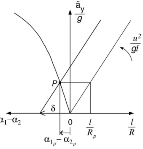
param-eters of the vehicle (curve passing through the origin in Fig. 1.2). Equation (1.11) represents a straight line on the same plane, which depends on the two parameters u and δ (straight line on the left in Fig. 1.2). Once the values of these parameters have been assigned, the intersection point between the line and the curve represents the corresponding equilibrium condition of the vehicle in the cornering manoeuvre defined by the actual values of u and δ (point P in Fig. 1.2). The curve described by equation (1.10) represents the handling curve.1

1_{In this brief summary of the single track model theory, only the main branch of}

the handling curve is examined. Such branch is obtained considering both the cornering characteristics Fy1(α1) and Fy2(α2) in correspondence to their increasing parts. Therefore, this is the branch of the handling curve which has the greatest practical relevance.

(26)

0 ã_y α₁−α₂ δ P α₁− α₂ p p g l R l R_p u gl 2

Figure 1.2: The handling diagram for the classical single track vehicle model.

Therefore, it has been demonstrated that, for the single track vehicle model, the difference between the front and rear slip angles (α1−α2) depends

only on the steady-state lateral acceleration ˜ay (see Fig. 1.2).

Two particular slip angles α1p and α2p correspond to a given equilibrium

condition P . Moreover, the corresponding value of the ratio l/Rp can be

obtained on the basis of equation (1.4). In Fig. 1.2, it is possible to use an auxiliary straight line, parallel to the line (1.11) and passing through the origin, and thus obtain the value of l/Rp on the rightwards axis.

According to [20], at each equilibrium condition the understeer gradient K is defined as K = d d˜ay µ δ − l R ¶ = d d˜ay (α₁− α₂) . (1.12)

Therefore, the understeer gradient K represents the slope of the handling curve at each equilibrium condition P .

The understeer-oversteer characteristics of the vehicle at each steady-state cornering condition P are defined as follows:

- understeer if K > 0; - neutral if K = 0;

(27)

- oversteer if K < 0.

Let us now introduce the cornering stiffnesses Φ₁ = dFy1 dα1 ¯ ¯ ¯ ¯ α1=α1p , Φ₂ = dFy2 dα2 ¯ ¯ ¯ ¯ α2=α2p , (1.13)

which represent the slopes of the cornering characteristics of the front and rear axles, evaluated at the slip angles α1p and α2p which correspond to a

given steady-state cornering condition P . The following relations can be obtained d˜ay dα1 = Φ1l a2m, d˜ay dα2 = Φ2l a1m. (1.14)

Therefore, the understeer gradient K is given by

K = m l µ Φ₂a₂− Φ₁a₁ Φ1Φ2 ¶ . (1.15)

Summing up, for the classical single track vehicle model the handling diagram depends only upon the constructive features of the vehicle. Ac-cordingly, the understeer gradient depends only on the steady-state lateral acceleration ˜ay, and therefore on the steady-state cornering condition (point

P in Fig. 1.2). Therefore, the handling diagram and the understeer-oversteer characteristics do not depend on the particular manoeuvre performed. As it will be demonstrated, these results are valid only for the very particular single track model since, in general, there is a strong dependence on the manoeuvre.

1.3 Model of a vehicle with locked differential

A rear-wheel drive vehicle fitted with a locked differential is now considered. As shown in Fig. 1.3, also in this case the motion of the vehicle is assumed to be plane and parallel to the road, which is horizontal and perfectly even. Therefore, the model has three state variables: the longitudinal speed u, the lateral speed v and the yaw rate r, which have the same meanings of the state variables u, v and r introduced for the single track vehicle model. The reference frame attached to the vehicle, whose versors are (i, j, k), is also the

(28)

same for this vehicle model and the single track model. Therefore, also in this case the following relations hold

VG= u i + v j,

aG= dV_dtG = ( ˙u − vr) i + ( ˙v + ur)j = ax i + ayj,

where VG and aG are the speed and the acceleration of the centre of mass

G, respectively, a_x is the longitudinal acceleration and a_y is the lateral ac-celeration. The yaw rate r is the only component of the angular velocity of the vehicle Ω, as in the single track model: Ω = r k.

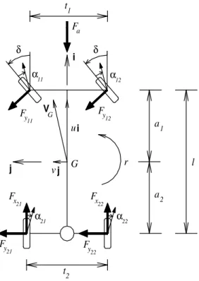
The meanings of the symbols in Fig. 1.3 and 1.5 are as follows. Some of them have been already introduced in the preceding section for the single track vehicle model. The parameters a1and a2 are the longitudinal distances

between the centre of mass G and each axle, l = a1+ a2 is the wheelbase, t1

and t2 indicate the front and rear tracks, respectively, δ is the steer angle of

the front wheels. Small steer angles are assumed, i.e. δ ≤ 15◦_{, thus allowing}

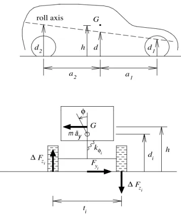
for the following approximations: sin δ ' δ, cos δ ' 1. As a consequence, left and right steer angles are assumed to be almost equal. Moreover, there is no steering in the rear wheels. The distance h is the height of the centre of mass, while d1, d2and d are the heights of the roll axis measured respectively

at the front axle, at the rear axle and at the centre of mass.

As opposite to the single track model, for a vehicle fitted with a locked differential there is the need to define a model with four wheels. In Fig. 1.3 the wheels of the vehicle are identified by means of the indices ij: the index i refers to the axle (1: front; 2: rear), while the index j refers to the side (1: left; 2: right). As a consequence, longitudinal and lateral forces acting on the tyres are respectively named F_x_ij and F_y_ij. No longitudinal force acts on the front tyres, since the rolling resistance is neglected. The self aligning torques on all tyres are also neglected. The force Fa = ρSCxu2/2 is the

longitudinal component of the aerodynamic drag force, where ρ is the air density, S is the frontal area of the vehicle and Cx is the aerodynamic drag

coefficient. The effects of the aerodynamic forces on the lateral and yaw equilibrium equations are neglected.

In the following paragraphs, the vehicle model will be defined by means of four sets of equations: the equilibrium equations, the congruence equa-tions (tyre theoretical slips), the constitutive equaequa-tions (tyre model) and the equations describing the vertical load acting on each tyre.

(29)

α α 22 y F y₂₁ t₂ F F j G r 21 21 α x v j 22 22 α x F a₂ y G F 11 ui V 11 y F 12 1 a 12 F δ i a t₁ δ l

Figure 1.3: Kinematics and force definition of the vehicle model with locked differential.

1.3.1 Equilibrium equations

Owing to all these hypotheses, the equilibrium equations of the vehicle are given by (Fig. 1.3)                m( ˙u − vr) = −(Fy11+ Fy12)δ + (Fx21+ Fx22) − Fa, m( ˙v + ur) = (F_y₁₁+ F_y₁₂) + (F_y₂₁+ F_y₂₂), J ˙r = (Fy11+ Fy12)a1− (Fy21+ Fy22)a2+ (Fx22− Fx21) t2 2 + (Fy11− Fy12) t1 2δ, (1.16)

(30)

where m and J are the vehicle mass and yaw moment of inertia with respect to the vertical axis k passing through the centre of mass G.

As it is common practice in classical vehicle dynamics ([8, 15, 30, 16]), it is possible to neglect the last term (Fy11 − Fy12)t1δ/2. Therefore the

equilibrium equations (1.16) become      m( ˙u − vr) = F_x₂ − F_y₁δ − F_a, m( ˙v + ur) = Fy1 + Fy2, J ˙r = Fy1a1− Fy2a2+ Mz2, (1.17) where Fx2 = Fx21 + Fx22, Fy1 = Fy11+ Fy12, Fy2 = Fy21+ Fy22, (1.18) and Mz2 = (Fx22− Fx21) t2 2. (1.19)

Having a locked differential requires the rear traction forces to be possibly different: Fx21 6= Fx22. Therefore, also the yaw moment Mz2 appears in the

yaw equilibrium equation. This is the only, but quite relevant, difference between equations (1.17) and the equilibrium equations (1.7) of the classical single track model.

As shown by many authors ([1, 17, 26, 25, 29, 33, 18, 10, 3, 4]) and by real applications for both commercial and sports cars, such a moment Mz2

strongly affects the cornering behaviour of vehicles. In the following sections, this aspect will be analyzed and discussed by means of a theoretical and systematic study.

1.3.2 Congruence equations: tyre theoretical slips

In order to analyze the effects of the tyre longitudinal slips on the steady-state cornering behaviour, a detailed theoretical description of the tyre kine-matics in combined slip conditions is necessary. Let σxij and σyij be the

longitudinal and lateral component of the theoretical slip σij (see e.g. [35])

of the tyre identified by the indices ij. Assuming a planar motion of the vehicle and small δ, these components are given by

(31)

• longitudinal theoretical slips: σx11 = ¡ u − rt1 2 ¢ + (v + ra1)δ − Ω11R1 Ω11R1 , σx12 = ¡ u + rt1 2 ¢ + (v + ra1)δ − Ω12R1 Ω12R1 , σx21 = ¡ u − rt2 2 ¢ − Ω21R2 Ω21R2 , σ_x₂₂ = ¡ u + rt2 2 ¢ − Ω₂₂R₂ Ω22R2 ; (1.20)

• lateral theoretical slips: σy11 = −¡u − rt1 2 ¢ δ + (v + ra1) Ω11R1 , σy12 = −¡u + rt1 2 ¢ δ + (v + ra1) Ω12R1 , σy21 = v − ra2 Ω21R2 , σy22 = v − ra2 Ω₂₂R₂ . (1.21)

In the above equations Ωij is the angular velocity of the generic tyre rim (see

Fig. 1.4), while R₁ and R₂ are the front and rear tyre rolling radii, which are assumed to be constant, thus neglecting their weak dependence on the vertical load.

It may be convenient to set Ω_ijR_i

u = 1 + χij, (1.22)

which defines the non-dimensional quantities χij.

Considering that under normal driving conditions the following relations hold |χij| ¿ 1, |r|t_i u ¿ 1, |r|a_i u ¿ 1, |v| u ¿ 1, |v ± ra_i| u ¿ 1, |δ| ¿ 1, (1.23)

(32)

the longitudinal and lateral slips may be given approximately by σx11 ' − µ χ11+rt_2u1 ¶ , σy11 ' −δ + v + ra1 u = −α1, σ_x₁₂ ' − µ χ₁₂−rt1 2u ¶ , σ_y₁₂ ' −δ +v + ra1 u = −α1, σx21 ' − µ χ21+rt_2u2 ¶ , σy21 ' v − ra2 u = −α2, σx22 ' − µ χ22−rt_2u2 ¶ , σy22 ' v − ra2 u = −α2, (1.24)

where α1 and α2 are the slip angles of the front and rear axle (see Fig. 1.3

where, as usual, α11 ' α12' α1 and α21' α22' α2). Equations (1.24) are

linear relationships between the longitudinal and lateral slips of each tyre and v, r, δ and χij. They also show that χij do not affect the linearized

lateral slips.

For a rear-wheel drive vehicle with locked differential, the angular veloc-ities of the rear rims are the same (Ω21 = Ω22 = Ω2) and hence, according

to (1.22), χ₂₁ = χ₂₂ = χ. Moreover, the front tyre longitudinal slips σ_x₁₁ and σx12 are equal to zero, which means χ12= −χ11= rt1/(2u).

1.3.3 Constitutive equations: tyre model

We have now to relate the tangential forces acting on each tyre to the cor-responding theoretical slip; to keep the analysis as simple as possible, an isotropic tyre behaviour is assumed, as described in [35].

The forces acting on the generic tyre are shown in Fig. 1.4. In this figure, axes iw and jw lie on the road, which has been assumed to be perfectly even,

while axis k_w is orthogonal to the road. Assuming zero camber, the plane (iw, kw) coincides with the plane of the wheel. Let Ft and Fz represent the

total tangential force and the vertical load, respectively. The vector Ft lies

on the road and has two components: the longitudinal force F_x and the lateral force Fy. Neglecting any camber effect, the constitutive equation can

be written in the following form

Ft= −σ_σFt(σ, ∆Fz), (1.25)

where Ftis the magnitude of the total tangential force Ft, σ is the magnitude

(33)

F

_y t F j w j_w w i

F

_{x w}i

F

_zk_w k_w

Ω

Figure 1.4: Forces acting on the generic tyre.

respect to the static load F0

z. The longitudinal and lateral force components

are:

Fx = −σ_σxFt(σ, ∆Fz), Fy = −σ_σyFt(σ, ∆Fz), (1.26)

where σx and σy are the longitudinal and lateral slip components.

It is customary to employ the Magic Formula ([36]) for the definition of Ft(σ, ∆Fz) Ft(σ, ∆Fz) = Df sin ³ Cfarctan(Bfσ − Ef[Bfσ − arctan(Bfσ)]) ´ , (1.27) where Cf and Ef are suitable constants, while, as usual

D_f = µF_z = (q₁F_z+ q₂)F_z =£q₁(F_z0+ ∆F_z) + q₂¤ ¡F_z0+ ∆F_z¢, (1.28) B_fC_fD_f = q₃sin µ 2 arctanFz q4 ¶ = q₃sin µ 2 arctanFz0+ ∆Fz q4 ¶ , (1.29) do depend on ∆Fz, with q1 < 0, q2 > 0, q3 > 0, q4 > 0. The first relation

shows that the friction coefficient µ decreases with respect to the vertical load F_z, while the second relation shows that the tyre stiffness B_fC_fD_f

(34)

increases with respect to Fz if Fz < q4, and then lightly decreases as soon as

Fz > q4.

If a non-linear response of the tyre is considered, that is whenever large slip values are expected, the relationship (1.27) will be employed. However, if small tyre slips and small vertical load variations are assumed, it is possible to take only a few terms in the power series expansion of equation (1.27) around the point (σ = 0, ∆Fz = 0), obtaining the following expression

F_t(σ, ∆F_z) ' F_t(0, 0) + ∂Ft ∂σ ¯ ¯ ¯ ¯ 0,0 σ + ∂Ft ∂∆Fz ¯ ¯ ¯ ¯ 0,0 ∆F_z+ ∂2Ft ∂σ ∂∆Fz ¯ ¯ ¯ ¯ 0,0 ∆F_zσ = 0 + C0σ + 0 + k∆F_zσ = (C0+ k∆F_z)σ. (1.30) In the above equation C0 = ∂Ft

∂σ

¯ ¯

0,0 is the tyre stiffness at (σ = 0, ∆Fz = 0),

while k = ∂2Ft

∂σ ∂∆Fz

¯ ¯ ¯

0,0. Note that, if camber is considered to be negligible,

all the other second derivatives in equation (1.30) are zero.

According to equation (1.30), the total tangential force F_t is assumed to be a linear function of the theoretical slip σ, but with the tyre stiffness linearly dependent on the vertical load variation ∆Fz.

1.3.4 Vertical load on each tyre

There is now the need to evaluate the vertical loads acting on the four wheels of the vehicle. Under steady-state cornering conditions (i.e., ˙u = ˙v = ˙r = 0) it is reasonable to assume that the vertical load variation of each tyre is only due to the lateral load transfer.

For a vehicle with a locked differential, the steady-state lateral load trans-fer of each axle must be related not only to the steady-state lateral accel-eration ˜a_y = ur, as it is common practice in classical vehicle dynamics, but also to the yaw moment Mz2 (an aspect apparently first discussed in [11]).

In fact, by solving the last two equations in (1.17) for Fy1 and Fy2 under

steady-state conditions ( ˙v = ˙r = 0), we obtain Fy1 = m˜ay a2 l − Mz2 l , Fy2 = m˜ay a1 l + Mz2 l . (1.31)

According to Fig. 1.5, let us introduce the constants k_φ₁, k_φ₂ and k_φ, which are respectively the equivalent front axle, rear axle and vehicle roll stiffnesses

(35)

roll axis d₂ 2 a d h G a₁ d₁ h d_i t_i i F_y F_z ∆ i z F ∆ i φ kφ i G m ãy

Figure 1.5: Equilibrium conditions about the roll axis.

(k_φ= k_φ₁+ k_φ₂). The equilibrium equation about the roll axis (Fig. 1.5) for the sprung mass is given by

m˜ay(h − d) − kφφ = 0. (1.32)

Therefore, under steady-state cornering conditions the roll angle of the sprung mass is

φ = m˜ayh − d_k φ

. (1.33)

Finally, the equilibrium equations about the roll axis for the front and rear axles hold

F_y₁d₁− ∆F_z₁t₁+ k_φ₁φ = 0, (1.34) Fy2d2− ∆Fz2t2+ kφ2φ = 0. (1.35)

(36)

From the above equations, the following expressions for the lateral load transfers can be obtained

∆Fz1 = mB1ãy− Mz2 lt₁ d1 = mB1ãy− Fx22− Fx21 2lt₁ t2d1, ∆Fz2 = mB2ãy+ Mz2 lt2 d2 = mB2ãy+ Fx22− Fx21 2l d2, (1.36)

where the constants B1 and B2 are given by

B1 = _t1 1 µ a2 l d1+ k_φ₁ kφ(h − d) ¶ , B2 = _t1 2 µ a1 l d2+ k_φ₂ kφ(h − d) ¶ . (1.37) Note that some lateral load transfers may occur even at zero lateral acceleration, owing to the presence of the yaw moment M_z₂. As shown in the following sections, this is exactly what happens in manoeuvres with constant steer angle or with constant turning radius, in which the yaw moment Mz2

is not zero even when the lateral acceleration ˜a_y tends to zero. Finally, the vertical loads acting on the four tyres are

Fz11 = F 0 z11− ∆Fz1, Fz12 = F 0 z12+ ∆Fz1, Fz21 = Fz021− ∆Fz2, Fz22 = Fz022+ ∆Fz2. (1.38) The static loads F0

zij are assumed to be constant:

F_z0₁₁ = F_z0₁₂ = mga2 2l , F 0 z21 = F 0 z22 = mga1 2l , (1.39)

where g is the acceleration of gravity.

1.4 Vehicle model with linear tyre behaviour

In this section, a vehicle model with linear tyre behaviour is presented and discussed. The model is based on equilibrium equations (1.17), on linearized slips (1.24), on linearized constitutive equations (1.30) and on load transfers (1.36). Steady-state cornering conditions are considered in order to inves-tigate the effects of the locked differential on the handling diagram and on the understeer gradient.

Some relevant effects of several types of limited-slip differentials on the steady-state cornering behaviour of vehicles have been already described in

(37)

the technical literature ([17, 26, 25, 29, 18]). However, most authors have focused their attention on the influence of the constructive features of the differential on the cornering behaviour, without emphasizing the dependence of the handling diagram and the understeer gradient on the manoeuvre itself. In the following paragraphs a more general and systematic theoretical analysis of such a problem is proposed. Results for a more realistic vehicle model with non linear tyres will be presented in section 1.5.

1.4.1 Forces acting on the axles and yaw moment

According to equations (1.24), the lateral slips of the tyres belonging to the same axle can be considered equal. Therefore, the effects of the lateral load transfers ∆Fz1 and ∆Fz2 cancel each other and do not appear on the

expressions of the axle lateral forces defined in (1.18) Fy1 = Fy11+ Fy12 = 2C10 µ δ −v + a1r u ¶ = 2C₁0α1, F_y₂ = F_y₂₁+ F_y₂₂ = 2C₂0 µ −v − a2r u ¶ = 2C₂0α₂. (1.40)

On the contrary, the rear tyres do not have the same longitudinal slips and it is therefore necessary to consider the effect of the rear lateral load transfer ∆Fz2 on the axle (total) longitudinal force Fx2. Owing to the

de-pendence of the load transfer ∆Fz2 on the yaw moment Mz2, traction forces

acting on the rear wheels can be obtained by solving the following algebraic linear system                        Fx21 = −σx21(C20− k2∆Fz2) = µ χ +rt2 2u ¶ · C₂0− k2B2m˜ay− k2(Fx22− Fx21) d2 2l ¸ , Fx22 = −σx22(C 0 2+ k2∆Fz2) = µ χ −rt2 2u ¶ · C₂0+ k2B2m˜ay+ k2(Fx22− Fx21) d2 2l ¸ , (1.41) whose solution is

(38)

Fx21 = 1 4u2_{(l − d}₂_k₂_χ) h C₂0d2k2r2t22+ 2C20lt2ur − 2B2k2lmt2u2r2 +¡4C₂0lu2− 4B2k2lmru3− 4C20d2k2u2χ ¢ χ i , F_x₂₂ = 1 4u2_{(l − d}₂_k₂_χ) h C₂0d₂k₂r2t2₂− 2C₂0lt₂ur − 2B₂k₂lmt₂u2r2 +¡4C₂0lu2+ 4B2k2lmru3− 4C20d2k2u2χ ¢ χ i . (1.42)

Hence the rear longitudinal force Fx2 and the yaw moment Mz2 are given by

Fx2 = Fx21+ Fx22 = C20d2k2r2t22− 2B2k2lmt2u2r2+ (4C20lu2− 4C20d2k2u2χ)χ 2u2_{(l − d}₂_k₂_χ) , (1.43) Mz2 = (Fx22− Fx21) t2 2 = −C0 2lrt22u + 2B2k2lmru3t2χ 2u2_{(l − d} 2k2χ) . (1.44)

Finally, let R = u/r = u2_/˜a

y be the distance between the instantaneous

centre of rotation of the vehicle and the longitudinal vehicle axis. Note that in steady-state conditions R is also the turning radius. Considering that under normal driving conditions |χ| ¿ 1 and |r|ti

u ¿ 1, the following

approximate expressions for the rear longitudinal force F_x₂ and the yaw moment Mz2 can be obtained

Fx2 ' 2C20χ − C r uãy = 2C 0 2χ − C Rãy, (1.45) Mz2 ' µ A u2 + Cχ ¶ ãy = A_R + Cχãy, (1.46)

where A = −C₂0t2₂/2 and C = k2B2mt2. It is worth noting that the yaw

mo-ment Mz2 not only depends on the steady-state lateral acceleration ˜ay, but

also on other variables defining the vehicle motion, such as the longitudinal speed u, the variable χ and the turning radius R.

(39)

If the influence of the yaw moment Mz2 on the lateral load transfers ∆Fz1

and ∆Fz2 is neglected in equations (1.36), we will find exactly the same

approximate expressions shown in (1.45) and (1.46) for the rear longitudinal force Fx2 and the yaw moment Mz2 itself. Hence, for the present model such

a dependence has almost no effect on the vehicle dynamics. 1.4.2 Steady-state cornering behaviour

The steady-state equations of motion can be obtained by substituting ex-pressions (1.40), (1.45) and (1.46) in equations (1.17), with ˙u = ˙v = ˙r = 0                  −mvr = 2C₂0χ − Cr uur − 2C 0 1 µ δ −v + a1r u ¶ δ − 1 2ρSCxu 2_, mur = 2C₁0 µ δ − v + a1r u ¶ + 2C₂0 µ −v − a2r u ¶ , 0 = 2C₁0 µ δ − v + a1r u ¶ a1− 2C20 µ −v − a2r u ¶ a2+ µ A u2 + Cχ ¶ ur, (1.47) which, in a more compact form, can be rewritten as

     f₁(u, v, r, δ, χ) = 0, f2(u, v, r, δ, χ) = 0, f3(u, v, r, δ, χ) = 0. (1.48)

According to equations (1.47) or (1.48), five quantities fully describe the vehicle motion. Two of them need to be assigned, while the other three can be obtained by solving the algebraic equations (1.47). In some cases, it may be convenient to use different variables, such as the lateral acceleration ˜a_y or the turning radius R, by considering that ˜ay = ur = u2/R = r2R.

The first equation in (1.47) can be solved with respect to χ, obtaining the non linear relation

χ = −mvr + Cr uur + 2C10 µ δ −v + a1r u ¶ δ + 1 2ρSCxu2 2C0 2 , (1.49)

that shows that χ is strongly affected by the vehicle motion conditions. Moreover, we see that even with linear tyres, the overall vehicle model is non linear.

(40)

In order to obtain analytical expressions of the understeer gradient, the last two equations in (1.47) can be rewritten in the following form

(

m˜ay = 2C10α1+ 2C20α2,

0 = 2C₁0α1a1− 2C20α2a2+ Mz2,

(1.50) which provide the slip angles α1 and α2

α1 = ma₂ã_y − M_z₂ 2lC0 1 = ma2− (A/u 2_{+ Cχ)} 2lC0 1 ãy, α₂ = ma1ãy + Mz2 2lC0 2 = ma1+ (A/u2+ Cχ) 2lC0 2 ã_y. (1.51)

Accordingly, we obtain the important result δ − l R = α1− α2 = µ K₀+ Gχ + F u2 ¶ ˜a_y, (1.52)

where G and F are constants given by G = −1 2l C0 1 + C20 C0 1C20 C = −1 2l C0 1 + C20 C0 1C20 k2B2mt2, F = −1 2l C0 1 + C20 C0 1C20 A = 1 4l C0 1 + C20 C0 1 t2₂, (1.53)

and K0 is the understeer gradient of the classical single track vehicle model

with linear tyre behaviour

K0 = m_2lC 0 2a2− C10a1 C0 1C20 . (1.54)

For a compact rear-wheel drive passenger car, the following numerical values were found: K0 = 0.00333 s2/m = 1.87 deg/g, G = −0.0163 s2/m and

F = 0.519 m. For the same car, under normal driving conditions, the term Gχ is quite small.

Equation (1.52) shows that in a vehicle with a locked differential, the difference α1− α2 does not depend only on the lateral acceleration ˜ay, but

also on other variables which characterize the vehicle motion, such as the longitudinal speed u and the variable χ. This result has strong practical relevance.

(41)

As shown in the following sections by means of some classical manoeuvres (with constant forward speed, with constant steer angle and with constant turning radius), this aspect strongly affects the handling diagram and the understeer gradient K, which now has to be defined as the partial derivative

K = ∂ ∂˜ay µ δ − l R ¶ = ∂ ∂˜ay (α₁− α₂). (1.55)

Manoeuvres with constant forward speed

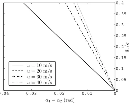
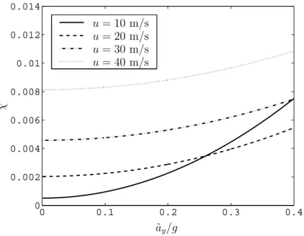
In these manoeuvres the forward speed u is assigned and kept constant. Some handling curves obtained in these manoeuvres for the very same vehicle are shown in Fig. 1.6, while the plots of the variable χ(u, ˜ay) and the yaw

moment M_z₂(u, ˜a_y) are shown in Figures 1.7 and 1.8, respectively.

Quite remarkably, in Fig. 1.6 we no longer have a single handling curve, as predicted by the classical theory for vehicles with open differential, but a

0 0.01 0.02 0.03 0.04 0 0.05 0.1 0.15 0.2 0.25 0.3 0.35 0.4 α₁− α2 (rad) ˜ay /g u = 10 m/s u = 20 m/s u = 30 m/s u = 40 m/s

Figure 1.6: Handling diagrams obtained with linear tyre behaviour in the manoeuvres with constant forward speed.

(42)

0 0.1 0.2 0.3 0.4 0 0.002 0.004 0.006 0.008 0.01 0.012 0.014 ˜ ay/g u = 10 m/s u = 20 m/s u = 30 m/s u = 40 m/s χ

Figure 1.7: Variable χ obtained with linear tyre behaviour in the manoeuvres with constant forward speed.

different curve for each velocity.

The corresponding understeer gradients Kucan be directly obtained from

equations (1.52) and (1.55) as Ku = ∂ ∂ãy µ· K0+ Gχ(u, ãy) + F u2 ¸ ãy ¶ = K0+ F u2 + G ·

χ(u, ˜ay) +∂χ(u, ˜ay)

∂˜ay ˜ay

¸ ,

(1.56)

where the function χ(u, ˜ay) is given by the solution (which can be obtained

employing some software for symbolic computation) of equations (1.47) with respect to v, δ and χ, after having set r = ˜ay/u.

We see that Ku is strongly affected by u and, particularly at low speeds,

it may be very different from K0. It is worth remarking that, with linear

tyres, the classical theory predicts a constant value K0 for the understeer

(43)

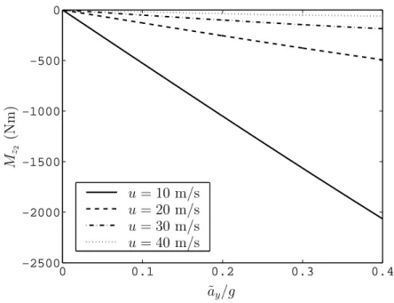
0 0.1 0.2 0.3 0.4 −2500 −2000 −1500 −1000 −500 0 ˜ ay/g u = 10 m/s u = 20 m/s u = 30 m/s u = 40 m/s M z2 (Nm )

Figure 1.8: Yaw moment Mz2 obtained with linear tyre behaviour in the

manoeuvres with constant forward speed.

Owing to the non linear dependence of χ on the forward speed u and on the lateral acceleration ˜ay, the understeer gradient does not decrease,

for increasing u, exactly with the square of the forward speed, although, in practice, the term G

h

χ(u, ˜ay) +∂χ(u,˜_∂˜_a_yay)˜ay

i

is quite small.

According to equation (1.52), the difference between the slip angles goes to zero if the lateral acceleration goes to zero

lim ˜ ay→0 (α1− α2) = lim ˜ ay→0 µ K0+ Gχ(u, ˜ay) + F u2 ¶ ˜ay = 0. (1.57)

As shown in Fig. 1.7, the variable χ(u, ˜ay) is always less than 0.012,

confirming the assumption |χ| ¿ 1. Note that the curves of χ do not pass through the origin if the forward speed is positive, even if the lateral accel-eration goes to zero (which requires δ → 0).

(44)

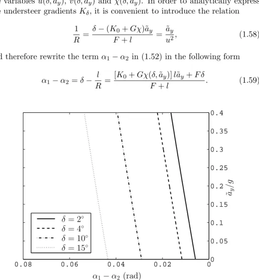
Manoeuvres with constant steer angle

The steer angle δ is assigned and kept constant. The handling diagrams and the plots of the yaw moment Mz2(δ, ˜ay) are shown in Figures 1.9 and 1.10,

respectively. Also in this case, the handling curve is not unique.

After having set r = ˜ay/u, equations (1.47) can be symbolically solved for

the variables u(δ, ãy), v(δ, ãy) and χ(δ, ãy). In order to analytically express

the understeer gradients Kδ, it is convenient to introduce the relation

1 R = δ − (K0+ Gχ)˜ay F + l = ˜ay u2, (1.58)

and therefore rewrite the term α1− α2 in (1.52) in the following form

α1− α2= δ −_Rl = [K0+ Gχ(δ, ã_{F + l}y)] lãy+ F δ. (1.59) 0 0.02 0.04 0.06 0.08 0 0.05 0.1 0.15 0.2 0.25 0.3 0.35 0.4 α1− α2 (rad) ãy /g δ = 2◦ δ = 4◦ δ = 10◦ δ = 15◦

Figure 1.9: Handling diagrams obtained with linear tyre behaviour in the manoeuvres with constant steer angle.

(45)

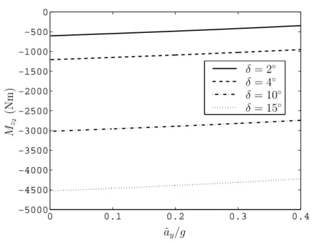
0 0.1 0.2 0.3 0.4 −5000 −4500 −4000 −3500 −3000 −2500 −2000 −1500 −1000 −500 0 ˜ ay/g M z2 (Nm ) δ = 2◦ δ = 4◦ δ = 10◦ δ = 15◦

Figure 1.10: Yaw moment M_z₂ obtained with linear tyre behaviour in the manoeuvres with constant steer angle.

Therefore the understeer gradients Kδ in manoeuvres with constant δ

be-come K_δ= ∂ ∂ãy µ δ − l R ¶ = K0+ G h χ(δ, ã_y) + ∂χ(δ,ãy) ∂ãy ãy i F + l l, (1.60)

which, again, are not equal to K0.

At low levels of lateral acceleration, the term G h

χ(δ, ˜a_y) + ∂χ(δ,˜ay)

∂˜ay ˜ay i

in equation (1.60) is quite small and the handling curves can be approximately considered straight parallel lines.

According to equation (1.59), the difference between the slip angles does not go to zero when the lateral acceleration vanishes, but it linearly increases with δ lim ˜ ay→0 (α₁− α₂) = lim ˜ ay→0 [K0+ Gχ(δ, ˜ay)]l˜ay+ F δ F + l = F F + lδ. (1.61)

(46)

Manoeuvres with constant turning radius

Finally, the turning radius R can be assigned and kept constant. The han-dling diagrams and the yaw moment Mz2(R, ˜ay) obtained are shown in

Fig-ures 1.11 and 1.12, respectively.

Equations (1.47) can be symbolically solved for the variables v(R, ã_y), δ(R, ãy) and χ(R, ãy) after having set u =

p

˜ayR and r =

p

˜ay/R (for a

turn in the leftwards direction, in which r > 0). It is convenient to rewrite α₁− α₂ in (1.52) in the following new form

α1− α2= δ −_Rl = [K0+ Gχ(R, ˜ay)] ˜ay+F_R (1.62)

which provides the understeer gradients KR in manoeuvres with constant

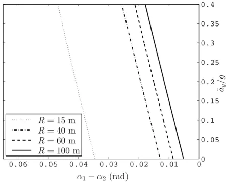
0 0.01 0.02 0.03 0.04 0.05 0.06 0 0.05 0.1 0.15 0.2 0.25 0.3 0.35 0.4 α1− α2 (rad) ˜ay /g R = 15 m R = 40 m R = 60 m R = 100 m

Figure 1.11: Handling diagrams obtained with linear tyre behaviour in the manoeuvres with constant turning radius.