Multibody analysis of a new three wheeled vehicle

(1)

Chapter 3

Tire models

The characterization of the tire is an important aspect in the multibody analysis of a vehicle. In fact each analysis has peculiar aspects that the tire model has to reproduce in a way, as close as possible, the reality. An handling analysis needs a tire model that has to reproduce the forces that the contact between tire and road produces. On the contrary, a tire model that has to be employed in a post rig analysis, has to represent the rapid variation of the vertical load.

3.1 Tire model used in handling analysis

A tire model that is employed in a handling analysis, has to represent, in an appropriate way, the contact forces that are generated on the interface between tire and road. In particular, Fig. 3.1shows these interaction forces, that can be summarized as follows:

• Fx: the brake/traction force;

• Fy: the cornering forces;

• FZ: the vertical tire load;

(2)

Figure 3.1: Forces and moments that are generated on the interface between tire and road

• My: the rolling resistance;

• Mz: the aligning moment.

ADAMS_°c

has the possibility to introduce tire models in the multibody model: the user can choose some tire model in function of the analysis that has to be performed. For this kind analysis, we chosen the PAC-MC Tire model, based on Pacejka ”Magic Formula”.

3.1.1 The tire magic formula: basic formulation

The ”Magic Formula” is a mathematical formulation that is capable of describing the basic tire characteristics for the interaction forces between the tire and the road under several steady-state operating conditions. We distinguish:

• pure cornering slip conditions: cornering with a free rolling tire: this is the example of a motorcycle running on a curve without drive torque;

(3)

3.1 Tire model used in handling analysis 35

• pure longitudinal slip conditions: braking or driving the tire without cornering;

• combined slip conditions: cornering and longitudinal slip simultane-ously. This is the more complex condition on a tire.

For pure slip conditions, the lateral force Fy as a function of the lateral

slip α, respectively, and the longitudinal force Fx as a function of

longitudi-nal slip κ. The basic Magic Formula equation is capable of describing this shape:

Y (x) = D sin [C arctan{BX − E(BX − arctan(BX))}] (3.1) where Y (x) is either Fx with x the longitudinal slip κ, or Fy and x the

lateral slip α.

The self-aligning moment Mz is calculated as a product of the lateral

force Fy and the pneumatic trail t

The figure, The Magic Formula and the Meaning of Its Parameters, illustrates the functionality of the B, C, D, and E factor in the Magic Formula:

• D-factor determines the peak of the characteristic, and is called the peak factor.

• C-factor determines the part used of the sine and, therefore, mainly influences the shape of the curve (shape factor).

• B-factor stretches the curve and is called the stiffness factor.

• E-factor can modify the characteristic around the peak of the curve (curvature factor).

(4)

(5)

3.1.2 The PAC-MC Tire model

Naturally the formulation introduced is a simplify version. In fact a good tire model has to describe these effects:

• combined slip condition. In combined slip conditions, the lateral force Fy decreases due to longitudinal slip or the opposite, the

longitudi-nal force Fx decreases due to lateral slip. The forces and moments

in combined slip conditions are based on the pure slip characteristics multiplied by the so-called weighting functions. Again, these weight-ing functions have a cosine-shaped.

• Transient tire behaviour: by introducing the relaxation length is pos-sible to characterize the transient.

• Inclination effects in the lateral force. From a historical point of view, the basic ”Magic Formula” has always been developed for car and truck tires, which cope with inclinations angles of not more than 10 degrees. To be able to describe the effects at large inclinations, an extension of the basic ”Magic Formula” for the lateral force Fy has

been developed in ADAMS_°c

.

So the PAC-MC Tire model developed in ADAMS_°c

, is able to represent these effects using a complex formulation in witch the input variables are:

• longitudinal slip κ.

• slip angle α [rad].

• inclination angle γ[rad].

• normal wheel load Fz[N]

Instead the output variables are:

(6)

Figure 3.3: The Magic Formula: inputs and outputs

• lateral force Fy [N].

• overturning couple Mx [Nm].

• rolling resistance moment My [Nm].

• aligning moment Mz [Nm].

To give an example, the magic formula for lateral force Fy and aligning

moment Mz in pure slip condition is quoted:

Fy0 = Dysin©Cyarctan{Byα − Ey[Byα − arctan(Byα)]}

ª

+ Cγarctan{Bγγ − Eγ[Bγγ − arctan(Bγαγ)]}

(7)

Where:

Cy = pCy1 λCy (3.3)

Dy = µy Fz (3.4)

µy = pDy1 exp(pDy2 ∆fz) (1 − pDy3 γ 2

y) λµy (3.5)

Ey = {pEy1+ pEy2 γ 2

y+ (pEy3+ pEy4 γy) sign(αy)} λEy (3.6)

Ky =pKy1 Fz0sin ( pKy2arctan · Fz (pKy3+ pKy4 γy2) Fz0 λF z0 ¸) (1 − pKy5γ 2 y)λF z0λKy (3.7) By = Ky/(CyDy) (3.8) Cγ= pCy2 λCγ (3.9) Kγ = (pKy6+ pKy7dfz) Fz λKγ (3.10) Eγ = pEy5 λEγ (3.11) Bγ= Kγ/(CγDy) (3.12) (3.13) Where:

• pCyn, pDyn, pEyn e pKyn are the coefficients that described the shape

of the curve;

• λCy, λµy, λEy, λKy, λCγ, λKγ e λEγ are scale factors.

The aligning moment Mz has the following formulation:

Mz= Mz0(α, γ, Fz) (3.14) Mz0= −t Fy0,γ=0+ Mzr (3.15) where: t(α) = Dtcos n Ctarctan [Btα − Et(Btα − arctan(Btα))] o cos(α) (3.16) Mzr(α) = Drcos[arctan(Brα)] cos(α) (3.17)

(8)

The coefficient introduced are described as follows: Bt= (qBz1+ qBz2 ∆fz+ qBz3 ∆f 2 z) (1 + qBz4γz+ qBz5|γz|) λKy/λµy (3.18) Ct= qCz1 (3.19) Dt= Fz (qDz1+ qDz2∆fz) (1 + qDz3 |γz| + qDz4γ 2 z) (R0/F_z0) λ_t (3.20)

Et=(qEz1+ qEz2 ∆fz+ qEz3 ∆f 2 z) n 1 + (qEz4+ qEz5 γz) µ 2 π ¶ arctan(BtCtαt) o (3.21) Br= qBz9 λKy/λµy (3.22) Dr =Fz (qDz6+ qDz7∆fz) λr+ (qDz8+ qDz9∆fz) γz + (qDz10+ qDz11 ∆fz) |γz| R0 λ_µy (3.23) Where:

• qBzn, qDzn e pEzn are the coefficients that describe the shape of the

curve;

• λµy, λKy e λt are scale factors.

The other forces and moments have a similar formulation.

the relaxation length σα (depending by the tire vertical load, the

incli-nation angle and the slip angle) is introduced in the tire model used by the following formulation: σα =pT y1sin ( pT y2 arctan · Fz (pT y3+ pKy4 γ2) Fz0 λFz0 ¸) (1 − pKy5 γ 2 ) R0 λ_Fz0 λσα (3.24)

The relaxation length modify the relation 3.2 and following formulation by introducing α′ _{instead of α:}

α′= arctan v σα

(9)

Figure 3.4: TNO tire test trailer

where v is the lateral deformation of the tire. This model used by ADAMS_°c

is very complex because the formula-tion introduced depends to many parameters that have to set up. These parameters are obtained generally by a test machine. The tire is tested in several conditions of slip angle, inclination angle, longitudinal slip. The data collected are elaborated to carry out the appropriate parameters to insert in the formulation. This series of operations is called ”tire character-ization”. The real tires that are fitted on Mp3 were characterized by TNO Automotive with a tire test trailer.

Fig. 3.4 shows the tire test trailer used by TNO to characterize the tires.

Figs. 3.5 and 3.6show the lateral force and aligning moment of the tire used in the handling analyses.

(10)

Figure 3.5: Tire lateral force Fy versus slip angle α, for several camber

angle γ

Figure 3.6: Tire aligning torque Mz versus slip angle α, for several camber

(11)

3.2 Three post rig tire model 43

Figure 3.7: Schema of the tire model used for three post analysis

3.2 Three post rig tire model

Respect to the previous tire model, this model is able to represent the variation of vertical loads when the scooter runs a bumpy road. So the tire model developed for the three post rig test has a more accurate definition of the vertical load by the use of an ADAMS_°c

build-in function. This model has one output: the vertical load FZ, in fact the three post rig test involves

only the vertical dynamics of the vehicle and therefore only the vertical load acting on the tire.

The tire was assimilate substantially to a spring-damper system (Fig. 3.7). So the tire is essentially described by a force between the connecting rod and the ground. This force is defined by the ADAMS_°c

routine ONE-SIDED IMPACT, that returns a real number for a force magnitude corresponding to a one-sided collision, using a compression-only nonlinear spring-damper formulation.

The arguments for this function are:

• displacement variable: a measure of the distance between colliding bodies; defined by a run-time displacement function.

(12)

• Velocity Variable: a measure of the time derivative of the distance between colliding bodies; defined by a run-time velocity function.

• Trigger for displacement variable: independent variable value at which to turn the one-sided impact on and off; defined by a real number, a run-time function, a design-time function, a design variable or an expression.

• Stiffness coefficient or K: stiffness coefficient for spring force; defined by a real number, a run-time function, a design-time function, a design variable or an expression.

• Stiffness force exponent: exponent for nonlinear spring force; defined by a real number, a run-time function, a design-time function, a design variable or an expression.

• Damping coefficient or C: damping coefficient for damper force; de-fined by a real number, a run-time function, a design-time function, a design variable or an expression.

• Damping ramp-up distance: distance over which to gradually turn on damping once impact is triggered; defined by a real number, a run-time function, a design-time function, a design variable or an expression.

Mathematically, IMPACT is calculated as follows:

max [0, K(q0− q)e− C ˙q ∗ ST EP ( ˙q, q0− d, 1, q0, 0)] (3.26)

where:

• q is the displacement variable;

• ˙q is the velocity variable;

(13)

3.2 Three post rig tire model 45

• Kis the stiffness coefficient;

• C is the damping coefficient;

• d is the damping ramp-up distance.

The function STEP is escribed in the following picture and approx-imates a step function with a cubic polynomial. Its calling function is represented by the following command:

ST EP (x, x0, h0, x1, h1) (3.27)

Where:

• x a double-precision variable that specifies the independent variable;

• x0 a double-precision variable that specifies the x value at which the

step function begins;

• h0 a double-precision variable that specifies the value of the function

before the step.

• x1 a double-precision variable that specifies the x value at which the

step function ends.

• h1 a double-precision variable that specifies the value of the function

after the step.

The formulation introduced allows to develop a tire model with a non linear vertical contact load.

First of all is necessary to build a force: in this case, for the front tires, it is applied to the connecting link (Fig. 3.10), for the rear tire directly to the rear hub.

The force is defined in this way: IMPACT( Def , Def speed ,R0 , S_t , 1

, Dt , 0.1).

Where:

(14)

Figure 3.8: Stiffness force of the Impact function versus the displacement variable q

Figure 3.9: Damping force of the Impact function versus the velocity vari-able ˙q

(15)

Figure 3.10: Three post rig test: the red arrow selected is the force defined by ONE-SIDE impact routine

• Def speed is the deformation speed;

• R0 is the rolling radius of the tire;

• Stis the stiffness of the tire;

• Stis the damping of the tire.

The parameters introduced by the formulation were set up using these two sources:

• the stiffness-damping characteristics of the tire fitted on the Mp3 measured with experimentation;

• a reference values implemented in the ONE-SIDE impact function. Fig. 3.11 shows a three post rig test: the red arrows represent the contact forces defined by the formulation introduced.

(16)

Figure 3.11: Three post rig test: the red arrows show the variation of the contact force defined by the ONE-SIDE impact routine

(17)

Chapter 4

Drivers developed

Another important objective of this research was to develop two drivers able to drive the motorscooter during the handling analysis. These two drivers can maintain the motorcycle stability by a different control strat-egy. The first one controls the steering angular speed of the handlebar, the second applies a steering torque on the handlebar. While the first one was directly developed in the ADAMS°c environment, the second, due to its complexity, was developed in the MATlAB/Symulink_°c

environment. This chapter explains only the control strategy of the two drivers. Physi-cally the body of the driver is fixed to the motorscooter frame by a fixed joint. The body is modeled by a sphere. ADAMS_°c

allows to customize the mechanic characteristics as weight and moments of inertia. These char-acteristics were set up to be as close as possible to an adult man of 75kg weight sat on the motorcycle saddle.

4.0.1 Steering speed driver

This driver controls the stability of the motorscooter by a steering speed. Fig. 4.1 shows the equilibrium of a motorcycle, in a steady state corner-ing manoeuvre. In particular we consider a simplified model of motorcycle in which the following effects are supposed negligible:

(18)

Figure 4.1: Equilibrium of a motorcycle

• the gyroscopic effects of the two wheels;

• the rolling resistance of the tires.

Furthermore we considered that the wheels can be represented by a disk with zero thickness and radius equivalent to the tire rolling radius. Behind these hypotheses, the only actions on the motorcycle are:

• the lateral acceleration ay

• the gravity acceleration g;

• the lateral tire load Fy;

• the vertical tire load Fz.

It is obvious that the system of these four forces must be balanced to assure equilibrium.

In particular we can write that:

mayH cos φ = mgH sin ˜φ (4.1)

(19)

51

• φ is the roll angle;˜

• H is the center of mass height.

During the steady state cornering manoeuvre the lateral acceleration ay

is:

ay =

u2

R (4.2)

Where:

• u is the forward speed;

• R is the radius of the curve.

Combining these two equations, we find that: ˜ φ = arctanµ u 2 R g ¶ (4.3) The 4.3 established a univocal relation between roll angle φ and the radius of the curve R. This result can be used to develop a control strategy: in fact the previous equation states that if the motorcycle is rolling by a roll angle ˜φ, the motorscooter is following a path of radius R. This is the result that is behind this control strategy. Let’s imagine that the motorcycle has to follow a pre-established path and let’s apply the control strategy before introduced. The first operation to do, is to obtain the radius of the path, or in a more appropiate way, the curvature of the path (the curvature of a path is the reciprocal of the path radius). When the curvature is obtained, trough the 4.3 it is possible to define the roll angle required for the trajectory. In particular in ADAMS°c environment, the curvature that the motorcycle has to follow, is given by a spline. In fact the input of this control strategy is only the curvature that we want the scooter to follow. This virtual driver is modeled directly in the ADAMS°c environment by a general motion applied on the handlebar (Fig. 4.3).

(20)

Figure 4.2: Graphic representation of ??

˙δ = −K1 ( ˜φ − φ) + K2 φ + K˙ 3 φ¨ (4.4)

Where:

• ˙δ is the angular speed of the handlebar, imposed by the general

mo-tion;

• φ is the desired roll angle defined by the 4.3;˜

• φ is the motorcycle roll speed;˙

• φ is the motorcycle roll acceleration;¨

• φ is the motorcycle roll angle;

(21)

53

Figure 4.3: Steering speed driver represented by a general motion

As we can see, this strategy of control, is based on the roll angle error that is defined as the difference between the desire roll angle and the actual roll angle of the motorcycle.

This is a simple, but very efficiency control strategy.

The drive/brake control is described in the following section, in fact the control strategy is the same, even if in this case it was directly implemented in ADAMS_°c

environment.

4.0.2 Torque driver

This virtual driver was developed though the model proposed in [6]. In par-ticular this driver is a control system able to drive a motorscooter, searching to avoid the falling and the intrinsical instability of the motorcycle. The virtual driver has in input a pre-established trajectory and gives in output the steering torque. The driver is able to control the longitudinal speed of the motorscooter by a drive/brake system.

(22)

The control system was developed in MATLAB/Simulink_°c

environ-ment: through this powerful tool, it was possible to develop the control strategy. In this environment was developed the driver that returns to ADAMS the steering torque: in fact while the motorcycle dynamics is de-termined by ADAMS_°c

, MATLAB_°c

provides the control variables to avoid the fall. The two softwares can dialogue through a block (orange in Fig.4.4): this is the interface module that allows the variables exchange.

In particular Fig. 4.5 shows the input/output variables of the control interface between the two softwares. However it is possible to see, the variables that the driver provides to ADAMS_°c

are:

• the steering torque that is modeled in ADAMS_°c

environment by a one component torque;

• the drive/brake control to maintain a pre-established speed. The steering torque is defined by the following law:

Ts= K0φ + K¨ 1φ + K˙ 2∆φ + K3∆ψ + K4∆p (4.5)

where:

• φ is the roll acceleration;¨

• φ is the roll speed;˙

• ∆φ is the roll error, defined like the difference between the actual roll angle of the motorscooter and the roll angle required φd. This last is

defined with the follow relation: φd= arctan(u

2

C/g) (4.6)

where u is the longitudinal speed, C is the curvature of the path, g the gravity acceleration;

• ∆ψ is the yaw error between the actual yaw angle and the yaw angle required (Fig. 4.7);

(23)

55

(24)

Figure 4.5: Control interface between Matlab_°c

and ADAMS_°c

• ∆p is the position error between the position required and the actual position of the motorscooter. This is defined like the minimum dis-tance (point P) from the path of the point N (projection at the road plane of the motorcycle center of mass, along the longitudinal plane Fig. 4.6).

The yaw, roll and position errors are calculated as follow. The input of the Matlab/simulik_°c

control strategy is a predefined path. In particular MATLAB_°c

loads a two column matrix in which each row, is a point of the trajectory. Then abscissa is defined: each point of the path is associated to a curvilinear abscissa that follows the trajectory from the start to the end. So each point of the path is well identified by its abscissa. The next step is to define the yaw angle required, this is defined by the following relation:

ψ = atan(Dy/Dx) (4.7)

(25)

57

Figure 4.6: Motorcycle and its coordinate systems

(26)

• Dx is the change ordinate of two points of the path,

• Dy is the delta along the y.

This way is generated a vector that represent the yaw angle that the motorcycle has to follow along the trajectory. So each row of the yaw vector is associated to a point of the path and that is associated to the abscissa.

Following this method it is possible to associate to each abscissa a value of roll angle if it is calculated to the curvature of the path.

When the simulation is started, Simulik_°c

, for each step, finds the min-imum distance point of the trajectory from the N point: in this way it defined the error position from a reference point. This point is associate to a curvilinear abscissa that returns the yaw angle and roll angle required: the control strategy can give a value of steering torque.

The control of longitudinal speed is demand to a traction force applied at the rear hub, and (to assure the equivalency of the real system of forces), also the transport torque. This system of forces can accelerate or brake the motorscooter to maintain a desired longitudinal speed, or a required profile of speed.

The longitudinal speed can be control by two components of the vector force in respect to the absolute reference system. These are described by two single component forces: one in the x direction Ftx), one in the y

di-rection (Fty). These two forces are defined to maintain the resultant force

always conducted directly along the longitudinal plane of the motorscooter. Furthermore any variation of inclination angle can influence the longitudi-nal force.

The two components were defined by the following formulation:

Ftx= cos(ψ) Z ˙ Ft dt (4.8) Fty = sin(ψ) Z ˙ Ft dt (4.9)

(27)

Where:

˙

Ft= A (˜un− un) − B ˙un (4.10)

in which:

• u˜n is the longitudinal speed desired;

• un is the actual longitudinal speed;

• ˙unis the longitudinal acceleration derived from the longitudinal speed

;

• A e B are opportune parameters;

• ψ is the yaw angle of the motorscooter.

The transport torque has the following formulation: Mt= HCr

Z ˙

Ftdt (4.11)

where HCr is the height of the center wheel. The second term of the 4.10

(28)

(29)

Chapter 5

Kinematic analysis of the

front tilting system

The front design is the real innovation of this motorscooter. Two front wheels mean to have two contact points and this is a new condition for a motorscooter: the kinematics is changed in respect to a traditional motor-cycle. Furthermore the changing of the kinematic quantities, implies also a changing of the contact forces. So a kinematic analysis of the front design can be useful to understand these aspects. In particular, due to the con-strain configuration, we have to expect a movement of the contact points during cornering. In this chapter will be investigated how the displacement of the contact points can be affected by roll and steering movements.

5.1 Description of the analysis performed

The front tilting system was analyzed in a deep way to characterize the kinematic behaviour.

In particular the forecarriage including the tires, was disconnected from the frame and the rear part. The tires were considered like a rigid part without stiffness. The tires were represented by two toroids to assure a

(30)

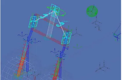
Figure 5.1: Joints configuration for the tilting system kinematic analysis

well determined contact point between tire and road. In fact the analysis was aimed to characterize the displacement of the two contact points when motorcycle roll angle and steering angle vary. In the disconnection point to the fame a planar joint was inserted to avoid the fall of the tilting system and to allow the rolling movement (Fig. 5.1).

Furthermore the contact between road and tires were modeled by the ADAMS CONTACT function. This function generates two forces between the two elements:

• a normal force (normal to the common plane of the two curvatures in the contact point). Its magnitude is obtained from the IMPACT function,

(31)

5.2 Results obtained 63

This last one is described from the following parameters:

• static coefficient;

• dynamic coefficient;

• stiction transition velocity: is the velocity above that the adhesion coefficient has the same value of the dynamic coefficient;

• friction transition velocity: is the velocity behind that the adhesion coefficient has the same value of the static coefficient.

The parameters used are shown in Fig. 5.2.

Using the model described above was characterized the displacement of the two front contact points varying the roll angle and the steering angle. In particular it was considered a + − 45 degree roll angle range and a 0 − 6 degree steering angle range, combined between them.

5.2 Results obtained

Fig. 5.3 shows the results obtained from the analysis. The graph shows the magnitude of the longitudinal displacement of the wheel contact point versus roll angle of different steering angle.

The longitudinal displacement was calculated like the displacement of the contact point in respect to a fixed ground marker (the initial position of the contact point before the displacement). In particular the CONTACT ADAMS_°c

function is able to return the displacement of the contact point and that is shown in the post processor environment.

5.3 Conclusions

The result presented in this chapter show::

• due to the design of the steering system and the tilting system, the two contact points, have a symmetric displacement: while one point of

(32)

(33)

Figure 5.3: Displacement of contact point

contact increases its longitudinal displacement, the second decreases the displacement. In particular, if the motorcycle runs on a curve: the inner point of contact goes back, and viceversa for the outer point. The maximum magnitude of the displacement can be evaluate about 40 mm.

• When the steering angle is null, the displacement is very close to a linear relation with the roll angle.

• The displacement influences the slip angle of the two wheels. The two front wheels have a track that causes two different front slip angles: in particular (cornering condition) the inner angle is bigger than the outer. But the displacement of the contact point increases the outer slip angle and decreases the inner: so the two wheels have almost the same slip angle, and they work in a closer condition.

(34)

(35)

Chapter 6

Three post rig analysis

In this chapter are presented the results from a three post rig test. Each tire of the motorscooter is put on plates that can move vertically. The plate movement reproduces a road profile that can be assume that the mo-torscooter runs with a constant forward speed on bumpy roads.

During the simulation the following quantities were observed:

• the vertical loads on tires;

• a saddle marker vertical acceleration;

• a saddle marker vertical displacement.

In particular the results obtained from the Mp3 motorscooter were com-pared with:

• the results obtained from a common motorscooter model;

(36)

Figure 6.1: Three post rig

6.1 Analysis procedure

Ideally every tire of the Mp3 were put on a plate that can traslate only with vertical movement (Fig.6.1). This movement reproduce a road profile. In particular a vertical displacement z(t) was applied at every plate: this was defined as follows:

z(t) = CUBSPL(t, u, 0, Roadprofile, 0) (6.1) Where:

• CUBSPL is an ADAMS function that gives a cubic interpolation ob-tained from a spline (in this case the spline is the argument ”road-profile”, or else a spline obtained from data referring to a real road profile) This function is formed by four arguments: the first one is the independent variable, the second argument is the second independent variable, the third one is the name of the spline, the fourth one is a number that represent the continuity order of the obtained curve.

(37)

6.1 Analysis procedure 69

• Roadprofile is the spline that describes the geometry of the road pro-file.

Three road profiles were used:

• road profile 1;

• road profile 2;

• a series of obstacles with a square section.

These road profiles are all real profiles, obtained from an experimenta-tion. In particular each profile is formed by two signals: one for the left, and one for the right wheel. The rear plate displacement was assumed the same of the right wheel but with the phase shifted of the motorcycle wheel-base.

The road profiles, before being imported in the ADAMS_°c

environment, were processed with a filtering algorithm. In particular the vertical dis-placement of the plate doesn’t match the vertical disdis-placement of the tire contact point (between tire and road). In fact the road profile contains spectral components of wavelength relatively small. If the wavelength is smaller then the tire rolling radius the geometry of the wheel represent a filter to the road profile. Fig. 6.2 shows how the contact point(where the vertical load is applied in the post test rig) doesn’t follow exactly the road profile. In particular the case shown in Fig. 6.2 represents a singularity for the contact point position.

So by the following simplification:

• camber angle null;

• rigid tire;

and using a simple algorithm, the road profiles were processed: the results were imported in the ADAMS°c _{environment and applied to the plates.}

(38)

Figure 6.2: Rigid wheel on a step

(39)

Figure 6.4: Graphical representation of filtering algorithm

• when the wheel is in contact with the road always a point of contact exists. This contact point is a point of the wheel.

• in the contact point the tangent to the wheel is the same for the road profile.

The conditions of contact are shown in Fig. 6.4.

These two conditions can be represented by two equations: dyp(xp) dxp = xp− xg yp− yg (6.2) (xp− xg) 2 − (yp− yg) 2 = r2 (6.3)

The equations 6.2 and 6.3 form a system that if solved gives the position of contact point (when yp and xp are known). In case of multiple solutions,

the contact point is the point with the lower yp.

(40)

Figure 6.5: Sample of unfiltered road profiles used for the simulations

(41)

• road profile;

• forward speed.

In particular for road profile 1 and 2, a forward speed of 30 km/h was used. Instead, for the obstacle test, the following forward speeds were used: 12, 24, 48, 60 Km/h.

The output data were:

• vertical tire loads;

• vertical displacement of a point close to the saddle;

• vertical acceleration of a point close to the saddle.

In particular for the tire loads was applied a RMS formula. For the standard motorscooter was used the following formulation:

∆F (t) = Ff(t) − Ff 0 (6.4) RM S = v u u t 1 n n X i=1 ∆F2_(t i) (6.5) Where:

• Ff(t) is the vertical load on the front wheel;

• Ff 0 is the static vertical load.

Mp3 has two front wheels, so the 6.4 was modified as follow:

∆F (t) = (Fr(t) + Fl(t)) − Ft0 (6.6)

Where:

• Fr(t) is the vertical load on the right wheel;

• Fl(t) is the vertical load on the left wheel;

(42)

0.950 1 1.05 1.1 1.15 1.2 1.25 1.3 1.35 1.4 500 1000 1500 2000 2500 3000 Time [s] Multybody Analytical

Figure 6.7: Road profile 1. Tire rear vertical load versus time simulation, forward speed 30km/h

6.2 Results

This section present only a significant samples of the results obtained from simulations. Figs 6.7, 6.8, 6.9, 6.10, 6.11 and 6.12 shows the comparison between the multibody model and the analytical model.

(43)

6.2 Results 75 0.950 1 1.05 1.1 1.15 1.2 1.25 1.3 1.35 1.4 500 1000 1500 2000 2500 Time [s] Multibody Analytical

Figure 6.8: Road profile 1. Tire right vertical load versus time simulation, forward speed 30km/h 1 1.05 1.1 1.15 1.2 1.25 1.3 1.35 1.4 −5.5 −5 −4.5 −4 −3.5 −3 −2.5 −2 −1.5 −1 Time[s] Multiboby Analytical

Figure 6.9: Road profile 1. Vertical displacement of the saddle point versus time simulation, forward speed 30km/h

(44)

0.95 1 1.05 1.1 1.15 1.2 1.25 1.3 1.35 1.4 −6 −4 −2 0 2 4 6 Time [s] Vertical acceleration [m/s 2] Multibody Analytical

Figure 6.10: Road profile 1. Vertical acceleration of the saddle point versus time simulation, forward speed 30km/h

Ex. A. M. Error % analytical Error % multibody Road profile 1 764 836 829 9.42 8.51

Road profile 2 919 985 991 7.18 7.83

Table 6.1: RSM value of the vertical tire load for profile1 and profile2. Ex.=experimental data, M.=multibody and A.=analitycal

Forward speed m/s Ex. A. M. Error % A Error % M 3.3 231 241 246 4.3 6.5 6.6 361 361 363 0.0 0.0 13.3 494 464 469 -6.1 -5.1 16.6 419 414 415 -1.2 -1.0

Table 6.2: RSM value of the vertical tire loads for series of obstacle. Ex.=experimental data, M.=multibody and A.=analitycal

(45)

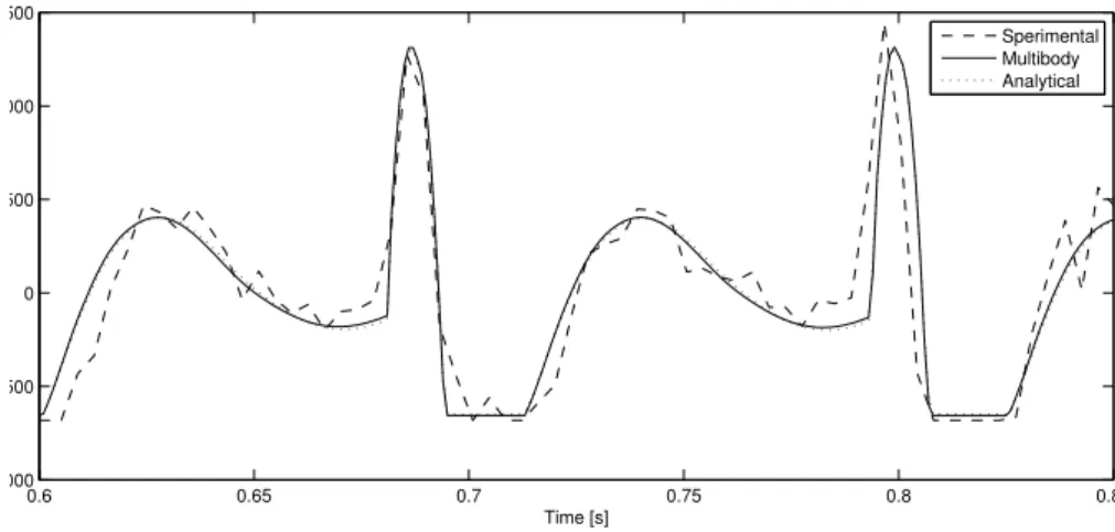
6.2 Results 77 0.6 0.65 0.7 0.75 0.8 0.85 −1000 −500 0 500 1000 1500 Time [s] Sperimental Multibody Analytical

Figure 6.11: Serie of obstacles. Vertical right tire load versus time simula-tion, forward speed 48km/h

Experimental (two wheels) Road profile 1 936

Road profile 2 1496

Table 6.3: RSM value of the vertical tire loads for profile1 and profile2, experimental data, two wheeled vehicle

Forward speed m/s Experimental (two wheels)

3.3 413

6.6 628

13.3 792

16.6 836

Table 6.4: RSM value of the vertical tire loads for series of obstacle, exper-imental data, two wheeled vehicle

(46)

0.6 0.65 0.7 0.75 0.8 0.85 −300 −200 −100 0 100 200 300 400 Time [s]

Figure 6.12: Series of obstacles. Vertical left tire load versus time simula-tion, forward speed 48km/h

6.3 Conclusions

The results presented in this chapter, show:

• a good agreement between multibody and analytical model. In fact both the models return results that are very close.

• a good agreement between models and experimental data. The mod-els are able to represent many aspects of the real vehicle.

• Regarding the comparison between a standard motorscooter and the Mp3, it can be noticed the advantage of two front wheels. In fact all the simulations and the experimental tests show that t heMp3 has a lower value of RMS. This means that the variation of the vertical load of the forecarriage is limited.

(47)

Chapter 7

Handling simulations

Handling tests are commonly used to characterize the dynamic behaviour of a vehicle. From these analyses, it is possible to obtain results that can define the behaviour of the vehicle

In general several standard manoeuvres are used to characterize the dynamics, such as:

• steering pad: the vehicle runs on a circular path of a established radius at constant forward speed;

• lane-change: the vehicle changes position laterally from a roadway lane to a parallel lane, at constant forward speed ;

• slalom: the vehicle zigzags between obstacles.

These maneuvers can be simulated in the ADAMS_°c

environment, and through the post-processor it is possible to obtain the following quantities:

• lateral acceleration of the vehicle;

• steering torque;

(48)

• roll angle;

• slip angles;

• tire forces.

the dynamic behaviour of the vehicle can be characterize analyzing these variables. The drivers models able to avoid the falling and to control the motorscooter were introduced in chapter three.

The following section shows the results obtained from the simulation of these common manoeuvrers obtained from the analytical model and the multibody model of the Mp3. So it was possible to validate the models against each other. Furthermore Piaggio provided some results from a handling experiment; in particular these results were compared to the data obtained from the multibody model.

7.1 Steering pad test

The following subsection describes the results obtained from the steering pad test. In particular the data obtained from the Mp3 multibody model were compared to data obtained from:

• the two standard wheeled multibody model;

• the analytical model;

• experimental data provided by Piaggio.

In the steering pad test the vehicle follows a circular path with an es-tablished radius and longitudinal forward speed. This condition represents a steady state for the vehicle. In order to perform this simulation two circle path of 100 and 50 meters radi and two forward speed of 10 and 20 m/s were chosen. For comparison with experimental data a 30 meters circular path and several forward speed were chosen. Fig. 7.1 shows one of the path used for this test (50 meters radius). Specifically the vehicle starts its run on a straight path to stabilize the longitudinal forward speed and

(49)

7.1 Steering pad test 81

the motion of the suspension. Then the vehicle starts to steer in to the circular path, and when the magnitude of lateral acceleration is stable, the following quantities were recorded :

−40 −20 0 20 40 60 80 −90 −80 −70 −60 −50 −40 −30 −20 −10 0 10 Steering pad [m] [m]

Figure 7.1: Path used for the steering pad test: 50 meters radius

• vehicle roll angle;

• front and rear slip angles;

• steering angle;

(50)

Front tire Rear tire φ [deg] δ [deg] α1_i [deg] α2 [deg]

Mp3 6.3 0.77 0.44 0.32 Two wheels 6.3 0.63 0.55 0.3

Table 7.1: Comparison of the Mp3 model and standard two wheeled model: steering pad 100m radius, forward speed 10 m/s, φd 5.8 deg

Mp3 24 0.74 1.36 1.27 Two wheels 23.8 0.3 1.7 1.17

• tire lateral force;

• tire aligning moment.

7.1.1 Mp3 multibody model versus standard two wheeled

motorscooter

This subsection compares the data obtained form the simulation performed with the Mp3 model and the results obtained with a traditional motorscooter multibody model. Tables 7.1, 7.2, 7.3, 7.4 show the comparison.

Mp3 12.4 1.57 0.85 0.66 Two wheels 12.4 1.3 1 0.61

(51)

Mp3 41.5 1.1 1.2 0.85 Two wheels 41.5 0.8 1.51 0.86

The value of the standard motorscooter front slip angle is a little bit higher with respect to that of the Mp3. This depends on the cornering and camber stiffness of the tires used. Specifically Fig. 7.2 and 7.3 show normalized camber and cornering stiffness versus tire vertical load (we want to remember that each front wheel of the Mp3 have a vertical load that is about halved with respect to the standard motorscooter multibody model). The variation of normalized cornering stiffness is higher than the normalized camber stiffness, so it causes an higher slip angle.

(52)

Figure 7.3: Normalized cornering stiffness versus vertical tire load

7.1.2 Mp3 multibody model versus analytical model

In this subsection the results obtained with the multibody model are com-pared with the results obtained with the analytical model. Tables 7.5, 7.6, 7.7, 7.8 show the comparison.

multibody 6.3 0.77 0.44 0.32 analytical 6.4 0.78 0.45 0.33

Table 7.5: Comparison of the Mp3 multibody model and analytical model: steering pad 100m radius, forward speed 10 m/s, φd 5.8 deg

(53)

multibody 24 0.74 1.36 1.27 analytical 24.3 0.75 1.4 1.3

7.1.3 Multibody model data versus experimental data

This subsection compares experimental data to the results obtained with the multibody model under the same test conditions. In particular the path radius is 15 meters. During the experimental test it was asked to the driver to follow a circular trajectory at various speeds: 20, 30 and 35 Km/h. It was also possible to record some of the quantities introduced in the previous sections, and after processing, these were compared with the results obtained from the multibody model.

(54)

Figure 7.4: Roll angle versus time: multibody data compared to experi-mental data, forward speed 30km/h

Figure 7.5: Steering angle versus time: multibody data compared with experimental data, forward speed 30km/h

(55)

Figure 7.6: Steering torque versus time: multibody data compared with experimental data, forward speed 30km/h

The Figg. 7.7, 7.8, 7.9 show the results obtained with a forward speed of 35km/h

(56)

Figure 7.7: Roll angle versus time: multibody result compared with exper-imental data, forward speed 35km/h

Figure 7.8: Steering angle versus time: multibody result compared with experimental data, forward speed 35km/h

(57)

7.2 Lane change test 89

Figure 7.9: Steering torque versus time: multibody result compared with experimental data, forward speed 35km/h

7.2 Lane change test

A lane change manoeuvre at 20m/s forward speed was also performed . The path is represented in Fig. 7.10. The comparison of the results obtained from the multibody model and the analytical model are show in Figg. 7.11, 7.12 and 7.13.

(58)

Figure 7.10: Trajectory of the lane change manoeuvre

Roll angle [deg]

(59)

7.2 Lane change test 91

Steering angle[ deg]

Figure 7.12: Steering angle of the lane change manoeuvre

Steering torque [deg]

(60)

7.3 Slalom test: multibody model data versus

ex-perimental data

This section compares the experimental data and the results obtained from the multibody model in the slalom test. The path of the slalom is shown in Fig. 7.14

Figure 7.14: Experimental slalom path

The results are shown in Figs. 7.15, 7.16, 7.17 and 7.18. Fig. 7.18 shows the forward speed of the vehicle in particular.

(61)

7.3 Slalom test: multibody model data versus experimental data 93

Figure 7.15: Roll angle versus time: multibody data compared with exper-imental data

Figure 7.16: Steering angle versus time: multibody data compared with experimental data

(62)

Figure 7.17: Steering torque versus time: multibody data compared with experimental data

Figure 7.18: Forward speed versus time: multibody data compared with experimental data

(63)

7.4 Loss of grip test 95

Figure 7.19: Lateral forces in loss of grip test

7.4 Loss of grip test

An interesting test was performed: the loss of grip analysis. It was sup-posed that, during a steering pad test, one of the front tires suddenly lost grip. This is a condition that a driver can meet on the road: in fact dust or an oily patch can cause loss of grip. In particular this condition is simulated with a instantaneous redaction of the coefficient of adhesion between road and tire.

In this test the coefficient of adhesion of the left tire drops to a value of 0.1. So the steering pad test is performed with a longitudinal forward speed of 8.3m/s and a radius of 50m.

Figs. 7.19, 7.20 and 7.21 show the results of this test.

In particular, as it can see, the loss of grip happens between the fourth and sixth seconds of running. The lateral force of the left tire falls: this is due to the suddenly decrease of the coefficient adhesion value. The driver increases the steering angle in order to avoid falling, recovering lateral force

(64)

Figure 7.20: Steering angle in loss of grip test

(65)

with the right front tire. After the loss of grip, and the consequent transient, the vehicle returns to the required roll angle.

7.5 Conclusions

The following conclusions are derived from above:

• there is good agreement between multibody model and the analytical model results.

• there is good agreement between experiential data and the multibody model results

• the loss of grip test reveals a particular aspect that can increase the safety of the Mp3 with respect to a traditional motorscooter

(66)

(67)

Chapter 8

Conclusions

This work was aimed at characterizing the dynamic behaviour of the new scooter MP3 scooter by Piaggio. This scooter features two front wheels. A multibody model was built in the ADAMS_°c

environment. Two virtual drivers were develop to assure the stability of the motorcycle. The first steering torque to control the stability of the motorcycle, the second varies the rotation speed of the steering mechanism. The results obtained from the multibody model of the Mp3, were compared to results obtained from:

• an analytical model developed in the Mathematica_°c

environment. The objective of this strategy was to validate the analytical model though the comparison of the results obtained from both models. An-other objective was to develop a model of vehicle dynamics in order to identify characteristics that present critical influence on the dy-namics. In some cases ADMAS is a ”black box” and it is not possible to inspect equations and functions directly that govern the model’s behaviour. The analytical model is an ”open” model in wich the equations of motion can be inspected and edited. However ADAMS is a powerful tool: easy to use, fast in developing models and fast in simulating;

(68)

The following were performed to analyze the dynamics and kinematics of this motorcycle:

• an analysis of forecarriage kinematics: the relationship between the displacement of the two front contact points, the roll angle and steer-ing angle was investigated. The results show that the displacement of the two contact points modifies the slip angles of the two front wheels and influences the dynamics of the scooter.

• an analysis of handling: common manoeuvres were simulated. Specif-ically the following maneuvers were performed: steering pad, lane change and etc. Analysis of some characteristic quantities such as lateral acceleration, steering torque and slip angles made it possible to characterize the dynamic behaviour of the Mp3. Furthermore, by comparing the results of the same tests carried out with a common motorscooter, it was possible to investigate the difference between the Mp3 and a standard motorcycle.

• Loss of adhesion during a steering pad test. Loss of adhesion on a front tire was simulated and the consequent dynamics were investi-gated. This analysis produced some interesting results in terms of diver safety: it was found if one of the front wheels loses grip, the other one reacts to assure the stability of the motorcycle.

• three post rig analysis. This test simulates the passage of the scooter over several bumpy road profiles. So saddle marker vertical accelera-tion and displacement were recorded and analyze.

A final remark about the finding of this research. This work was aimed at characterizing the dynamic behaviour of this new motorscooter, and to investigate the difference between it and a standard motorscooter. The analyses performed and their results do not demonstrate that the Mp3 is a better vehicle in all respect to a standard motorscooter. But it is evident that two front wheels can assure increased safety in some conditions.

(69)

List of main symbols

ay lateral acceleration m vehicle mass u longitudinal speed g gravity acceleration B stiffness factor C shape factor

C curvature of the path

Cα cornering stiffness

Cγ Camber stiffness

D peak factor

E curvature factor

Ft traction force

Fy lateral tire force

Fz vertical tire force

Fz0 nominal vertical tire force

Fx longitudinal tire force

H center of mass height

K stiffness coefficient

Mx tire overturning torque

My tire rolling resistance

Mz tire aligning torque

R path radius

(70)

α1 front slip angle

α2 rear slip angle

γ inclination angle

δ steering angle

µx longitudinal adhesion coefficient

φ roll angle ˙ φ roll rate ¨ φ roll acceleration ˜

φ required roll angle

ψ yaw angle

σα relaxation length

∆p position error

(71)

Appendix A

Sintesi in italiano

Summary in Italian

La ricerca svolta durante il triennio di dottorato, ha affrontato lo studio della dinamica di un nuovo veicolo a tre ruote introdotto nel mercato da Piaggio & C. S.p.A. nell’anno 2006. Il veicolo, chiamato Mp3 (Fig. A.1), presenta la particolare singolarità di avere due ruote anteriori che ne aumen-tano la stabilità di marcia, soprattutto su fondi stradali a bassa aderenza. Lo studio della dinamica di tale veicolo è doveroso: infatti mentre la dinam-ica dei motocicli convenzionali è già oggetto di studi approfonditi, questo non avviene per i veicoli innovativi a tre ruote come l’Mp3.

La caratterizzazione del comportamento dinamico del motociclo, `e avvenuta mediante la costruzione di un modello a corpi rigidi (modello multibody) sviluppato nell’ambiente di simulazione del codice MSC-ADAMS_°c

, soft-ware dedicato allo studio della dinamica si sistemi multi-corpo. Lo studio della dinamica `e stato svolto attraverso la simulazione di test, alcuni dei quali vengono regolarmente eseguiti per i motocicli convenzionali. In par-ticolare si sono eseguite le simulazioni dei seguenti test:

• prova al banco vibrante in modo da caratterizzare la dinamica verti-cale del mezzo;

(72)

Figure A.1: Nuovo scooter a tre ruote Piaggio & C. S.p.A

• test di handling, in cui sono state simulate alcune manovre standard.

Inoltre, data la peculiarit`a del sistema anteriore basculante, si `e eseguita un’analisi dello spostamento dei punti di contatto delle due ruote anteriori in funzione dell’angolo di rollio e dell’angolo di sterzo.

Nelle prove dove richiesto, si `e sviluppato anche dei controllori in grado di guidare il veicolo su di un percorso prestabilito, implementando non solo una strategia in grado di evitare la caduta, ma anche un sistema di trazione capace di inseguire un profilo di velocit`a desiderato.

I dati ottenuti dalle simulazioni sono stati comparati con quelli ottenuti da:

• un modello analitico sviluppato in ambiente Mathematica_°c

;

• un modello di scooter convenzionale, in modo da mettere in luce le differenze con un motorscooter standard;

(73)

105

• dati spermentali forniti da Piaggio & C. S.p.A..

Perch`

e due ruote anteriori?

In un’analisi preliminare possiamo affermare che due ruote anteriori portano i seguenti benefici:

• nell’usuale guida cittadina ci sono molti fattori che possono deter-minare la perdita dell’equilibrio di un motociclo: striscie bianche (spe-cialmente se bagnate da pioggia), tombini, buche del manto stradale. Due ruote assicurano una minore probabilità che tali fattori avvengano contemporaneamente su entrambe. Quindi se una ruota perde aderenza, l’altra può assicurare ancora la stabilità del mezzo.

• In accordo con la Magic Formula di Pacejka, il coefficiente di aderenza tra pneumatico e suolo, varia in funzione del carico verticale del pneu-matico. Il coefficiente longitudinale pu`o essere descritto attraverso la seguente formulazione: µx= p1+2 (Fz− Fz0) Fz0 (A.1) Dove:

– µx `e il coefficiente di aderenza longitudinale del pneumatico;

– Fz `e il carico verticale del pneumatico;

– Fz0 `e il carico nominale di prova del pneumatico;

– p1 e p2 sono parametri costanti sperimentali.

In particolare se il carico verticale aumenta, il coefficiente di aderenza diminuisce, poich`e il parametro p2 `e negativo. La figura A.2 mostra

il coefficiente di aderenza in funzione del carico verticale ottenuto con i parametri riferiti al pneumatico anteriore equipaggiato dall’Mp3. Le linee tratteggiate in figura fanno riferimento a due carichi verti-cali l’uno il doppio dell’altro. Considerando che ciascuna delle due

(74)

200 400 600 800 1000 1200 1400 1600 0.94 0.96 0.98 1 1.02 1.04 1.06 1.08 1.1 Fz adhesion coefficient

Figure A.2: Coefficiente di aderenza longitudinale in funzione del carico verticale. Parametri: p1 = 1, p2 = −0.1, F_z0 = 1000N

ruote anteriori dell’Mp3 supportano un carico circa la met`a di uno scooter convenzionale di pari categoria, appare evidente come si ab-bia un incremento del circa il 4-5%. Quindi l’anteriore ne guadagna in aderenza.

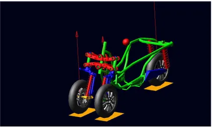
Architettura sistema basculante

La possibilit`a che ha Mp3 di essere guidato come un normale scooter deriva dall’innovativa architettura frontale (Fig. A.3). Il sistema basculante, com-posto da corpi vincolati tra loro in modo da formare un quadrilatero arti-colato, permette a Mp3 di rollare come uno scooter convenzionale, e quindi pu`o essere guidato senza stravolgere il normale stile la guida. La stessa architettura frontale ha integrato sia il sistema di sterzo, sia il sistema sospensivo di tipo a braccio spinto.

Una particolare attenzione si `e data allo studio di tale sistema. Si `e infatti caratterizzato lo spostamento longitudinale dei punti di contatto tra

(75)

107

(76)

Figure A.4: Modello multibody sviluppato

pneumatico e suolo stradale, in funzione dell’angolo di rollio e dell’angolo di sterzo del mezzo. Il risultato ottenuto è che durante la percorrenza di una curva, il punto di contatto del pneumatico interno arretra, mentre l’esterno avanza. Il risultato è molto interessante, infatti a causa della carreggiata dei due pneumatici anteriori, questi tenderebbero a lavorare con diversi angoli di deriva. Durante la percorrenza di un curva quindi, lo spostamento dei punti di contatto, fa in modo di diminuire tale differenza facendo lavorare i due pneumatici in una condizione più simile tra loro.

Modello multibody sviluppato

Per sviluppare il modello di veicolo ci si `e avvalsi del’utilizzo del codice com-merciale MSC-ADAMS_°c

: tale software `e in grado di integrare le equazioni del moto del sistema che viene modellato nel suo ambiente. La Fig. A.4 mostra il modello multibody sviluppato.

(77)

109

veicolo, tutti i singoli componenti cercano di ricalcare le caratteristiche di quelli reali. Quindi, utilizzando i disegni CAD tridimensionali, si sono ot-tenute le caratteristiche sia geometriche che inerziali dei vari corpi. Anche le caratteristiche elastiche e di smorzamento delle sospensioni sono state rica-vate direttamente da quelle reali e implementate direttamente nel modello. Una particolare attenzione `e stata data alla modellazione dei pneumatici. ADAMS_°c

permette di descrivere le forze e i momenti che si generano tra terreno e pneumatico, tramite un modello matematico che prende il nome di MF-tire, derivato direttamente dalla pi`u famosa Magic Formula di Pace-jka. Il pneumatico viene descritto tramite una formulazione matematica in cui numerosi parametri devono essere ricavati sperimentalmente. Tale caratterizzazione `e avvenuta tramite i laboratori del TNO Automotive.

Modelli di pilota sviluppati

Nelle prove in cui è stato necessario pilotare il mezzo, sono stati sviluppati due modelli di pilota virtuale. Indubbiamente ad un pilota è richiesto non solo di seguire un percorso predefinito, ma anche deve essere capace di in-seguire un profilo di velocità desiderato. In particolare sono stati sviluppati dei controllori:

• un controllore che agisce direttamente sullo sterzo tramite una coppia.

• un controllore che agisce sullo sterzo controllando la velocit`a di sterzo.

Pilota in coppia di sterzo

Il primo controllore sviluppato permette di controllare la coppia applicata allo sterzo, avente la seguente espressione:

Ts= K0φ + K¨ 1φ + K˙ 2∆φ + K3∆ψ + K4∆p (A.2)

Dove:

(78)

• φ `e la velocit`a di rollio del veicolo;˙

• ∆φ `e l’errore di rollio definito come la differenza tra l’angolo di rollio attuale del motociclo e l’angolo di rollio richiesto φd, calcolato secondo

la seguente relazione:

φd= arctan(u 2

C/g) (A.3)

dove u è la velocità longitudinale del mezzo, C è la curvatura del percorso, g l’accelerazione di gravità;

• ∆ψ `e l’errore di imbardata;

• ∆p `e l’errore di posizione.

In particolare tale controllore riceve in ingresso un percorso, da questo, tramite una serie di operazioni, vengono ricavati gli errori di posizione, imbardata e rollio.

La velocit`a longitudinale del mezzo `e controllata tramite un sistema di forze applicata al mozzo posteriore, e del conseguente momento di trasporto, per mantenere l’equivalenza con il vero sistema di forze di trazione, appli-cato nell’impronta di contatto.

Il pilota, a causa della sua complessit`a, `e stato sviluppato in ambiente Matlab-Simulink_°c

. ADAMS_°c

, attraverso una propria interfaccia perme-tte di interfacciarsi con Matlab_°c

attraverso un apposito blocco di comu-nicazione. Una schermata del pilota `e visibile in Fig. A.5dove il blocco arancio `e il blocco di comunicazione tra ai due ambienti: durante una co-simulazione Admas_°c

si occupa dell’integrazione delle equazioni del moto, invece Matlab°c _{fornisce le variabili che servono al controllo del mezzo.}

Pilota in velocit`a di sterzo

Il secondo controllore sviluppato controlla il veicolo attraverso l’imposizione della velocit`a di sterzo. Al manubrio viene applicata una velocit`a di sterzo avente la seguente espressione:

(79)

111

(80)

Figure A.6: Schema dell’interfaccia di controllo tra Matlab°c e ADAMS°c

˙δ = −K1 ( ˜φ − φ) + K2 φ + K˙ 3 φ¨ (A.4)

Dove:

• φ `e l’angolo di rollio desiderato;˜

• φ `e la velocit`a di rollio del motociclo;˙

• φ `e l’accelerazione di rollio del motociclo;¨

• φ ´e l’angolo di rollio del motociclo;

• K1, K2 e K3 sono parametri positivi costanti.

In particolare il controllore riceve in ingresso un profilo di rollio che deve essere inseguito: da qui, per ogni passo di integrazione, viene calcolato l’errore di rollio. Dalle equazioni di equilibrio in curva di un motociclo, `e possibile ricavare la seguente relazione:

(81)

113 φ = arctanµ u 2 nC g ¶ (A.5) Dove:

• φ `e l’angolo di rollio del motociclo;

• un`e la velocit`a longitudinale;

• C `e la curvatura del percorso;

• Rg `e l’accelerazione di gravit`a.

Quindi esiste una relazione univoca tra rollio e curvatura del percorso che il motociclo sta percorrendo. Sfruttando l’equazione appena introdotta è possibile quindi costruire una logica di controllo basata sull’errore di rollio. Tale pilota, molto più semplice del primo, è stato implementato di-rettamente all’interno dell’ambiente ADAMS_°c

. L’unico input di questa strategia di controllo è un profilo di rollio desiderato che il pilota insegue. Tale controllore è decisamente più semplice del primo, ma indubbiamente risulta essere di più facile gestione, specialmente nelle prove più semplici.

Simulazioni eseguite

Verranno ora presentate le simulazioni effettuate e i risultati ottenuti.

Prova al banco vibrante

Tramite questa prova si è potuto valutare le forze di contatto tramite suolo e pneumatico durante la percorrenza di tratti di strada accidentati. In questa simulazione ogni ruota del veicolo viene posizionata su di un piatto che può traslare verticalmente ricreando un profilo stradale. In particolare si è simulata la percorrenza di tre profili reali (Figg. A.9, A.10 ):

(82)

Figure A.7: Prova al banco vibrante

• un fondo acciottolato;

• l’attraversamento di tavolette quadrate.

I profili prima di essere utilizzati, hanno subito un processo di filtraggio. Infatti il profilo della superfice stradale sulla quale rotolano le ruote, può contenere componenti spettrali di lunghezze d’onda relativamente piccole. Se la lunghezza d’onda è più piccola o comunque è confrontabile con il raggio della ruota, la geometria della ruota stessa costituisce un filtro al profilo stradale. Infatti, come si nota in Fig. A.8, il punto di contatto C, in cui si considerano applicate le forze del terreno in tale prova, non segue fedelmente il profilo stradale, poichè il contatto tra terreno e pneumatico avviene in corrispondenza di un altro punto. Quindi, dato il profilo stradale e considerando la ruota rigida, si è calcolato lo spostamento verticale da applicare al punto C e quindi al piatto.

Le variabili che sono state monitorate durante le prove sono state:

• le forze verticali di contatto tra pneumatici e suolo. In particolare `e stato possibile calcolare il valore RMS della loro variazione rispetto al carico statico;

(83)

115

Figure A.8: Superamento di uno scalino da parte di una ruota rigida

• l’accelerazione verticale di un punto posto in corrispondenza della sella,

• lo spostamento verticale del punto sopra citato.

I risultati ottenuti dall prove sono stai direttamente confrontati con dati spriementali e con quelli ottenuti dal modello analitico. Alcuni risultati sono mostrati nelle figure seguenti (Figg. A.11, A.12).

In generale possiamo affermare che il modello riesce a descrivere in modo abbastanza fedele l’andamento dell forze di contatto: tale affermazione pu`o essere fatta alla luce del confronto con i dati sperimentali. Inoltre il modello matematico e modello multibody sono in buon accordo tra di loro. Con-frontando i dati con quelli provenienti dalla percorrenza degli stessi profili con uno scooter tradizionale si `e potuto osservare come, il sistema bascu-lante, porti dei vantaggi in termini di RMS delle forze di contatto anteriori che risulta essere inferiore per Mp3.

(84)

Figure A.9: Esempio dei profili di prova utilizzati nelle simulazioni

(85)

117 0.95 1 1.05 1.1 1.15 1.2 1.25 1.3 1.35 1.4 −6 −4 −2 0 2 4 6 Time [s] Vertical acceleration [m/s 2] Multibody Analytical

Figure A.11: Pav`e. Accelerazione verticale del punto sella, velocit`a di prova 30 km/h 0.6 0.65 0.7 0.75 0.8 0.85 −1000 −500 0 500 1000 1500 Time [s] Sperimental Multibody Analytical

Figure A.12: Tavolette. Forza verticale di contatto, velocit`a di prova 48 km/h

(86)

Simulazioni di handling

La simulazione di handling, tramite l’esecuzione di manovre standard, per-mette di valutare paramenti fondamentali per la caratterizzazione della dinamica del veicolo. In particolare grandezze importanti sono:

• le forze e i momenti scambiati tra suolo e pneumatico;

• l’accelerazione laterale del veicolo;

• l’angolo do sterzo del veicolo;

• la coppia di sterzo;

• l’angolo di rollio;

• gli angoli di deriva dei pneumatici.

Le manovre che si sono utilizzate per la caratterizzazione del mezzo sono state:

• steering pad, ovvero la percorrenza a velocit`a costante di un percorso circolare;

• cambio di corsia;

• inversione ad ”U”;

• slalom tra birilli.

Tutte le prove sopracitate sono state condotte a varie velocit`a longitu-dinali costanti. Indubbiamente tali prove permettono di avere un’ampia caratterizzazione della dinamica del mezzo, infatti `e possibile studiare sia la marcia dal veicolo in condizioni stazionarie, come nel caso dello steering pad, sia in condizioni di forte transitorio come lo slalom tra i birilli.

I dati ottenuti da tali prove sono stati sono stati direttamente con-frontati con quelli derivanti da prove sperimentali: in questo modo `e stato possibile avere una correlazione tra modello multibody e motociclo reale.

(87)

119

Figure A.13: Andamento del rollio in funzione del tempo per la prova di steering pad: raggio 15m, velocit`a 30 km/h

Di tutte le simulazioni effettuate riportiamo a titolo di esempio, i risul-tati ottenuti dalla manovra di steering pad eseguito a una velocit`a di 30 km/h su di un percorso circolare di raggio 15 m.

Una ulteriore analisi è stata la simulazione di perdita di aderenza da parte di una delle due ruote anteriori durante la percorrenza di una curva in condizioni di regime. In particolare si è simulata la rapida discesa del coefficiente di aderenza di uno dei pneumatici frontali. Il risultato ottenuto è che, dopo un breve transitorio, lo scooter si riporta sul percorso circolare che stava inseguendo prima della perdita di aderenza. Inoltre si può notare (Fig. A.16) come la ruota che perde aderenza ha un calo della forza laterale, mentre l’altra compensa aumentando la sua forza laterale.

Conclusioni

Con il lavoro presentato si `e caratterizzato il comportamento dinamico del nuovo scooter a tre ruote Paiggio Mp3. In particolare dalle prove svolte si `e potuto osservare che:

(88)

Figure A.14: Andamento dell’angolo di sterzo in funzione del tempo per la prova di steering pad: raggio 15 m, velocit`a 30 km/h

Figure A.15: Andamento della copia di sterzo in funzione del tempo per la prova di steering pad: raggio 15m, velocit`a 30 km/h

(89)

121

Figure A.16: Andamento delle forze laterali dei pneumatici anteriori in funzione del tempo per la prova di steering pad: raggio 20 m, velocit`a 30 km/h

specialmente su fondi sconnessi o in improvvise perdite di aderenza.

• il modello multibody sviluppato permette di simulare con sufficiente precisione la dinamica dello scooter Mp3. Tale affermazione `e sup-portata dal notevole accordo con i dati sperimentali.

• Il modello analitico ed il modello multibody sono in pieno accordo, quindi la validazione dei due modelli `e avvenuta avvicendevolmente. I due modelli, come in un primo approccio `e possibile pensare, non rappresentano la copia l’uno dell’altro, ma bens`ı due strumenti con caratteristiche differenti fra loro. Infatti, in una visione globale del la-voro svolto, i due modelli hanno lavorato sinergicamente per ottenere i risultati ottenuti.

(90)