Universit`
a degli Studi di Ferrara
Dottorato di Ricerca in
Fisica
Ciclo XXIII
Coordinatore Prof. F. Frontera
Critical Properties of the Potts Glass
with many states
Settore Scientifico Disciplinare FIS/03
Dottorando Tutori
Marco Guidetti prof. G. Fiorentini
prof. R. Tripiccione
[. . .] When I was a child I caught a fleeting glimpse Out of the corner of my eye [. . .] D. Gilmour, R. Waters
Contents
1 Overview 1
2 Introduction 5
2.1 A few initial pointers . . . 5
2.1.1 The order parameter . . . 5
2.1.2 The correlations . . . 6
2.1.3 Critical dimensions . . . 8
2.2 The Ising and Potts models . . . 8
2.2.1 The Ising model . . . 8
2.2.2 Mean Field Theory for the Ising model . . . 9
2.2.3 The critical exponents of the Ising model . . . 12
2.2.4 The Potts model . . . 14
2.2.5 Mean Field Theory for the Potts model . . . 14
2.3 Spin Glasses . . . 16
2.3.1 The Edwards-Anderson (EA) model . . . 17
2.4 How do we deal with disorder? . . . 19
2.4.1 The Replica Trick . . . 20
2.5 Broken Ergodicity, the Spin Glass phase and order parameters . . 21
2.5.1 Susceptibilities . . . 27
2.6 Frustration . . . 28
2.6.1 Trivial and nontrivial disorder . . . 29
2.7 A replica-symmetric approach . . . 31
2.8 Replica symmetry breaking: the Parisi solution . . . 37
2.9 The Potts Glass . . . 42
3 Monte Carlo Methods 47 3.1 A first glance . . . 47
3.2 Measures and Fluctuations . . . 49
3.3 Importance Sampling . . . 50 3.4 Markov processes . . . 51 3.4.1 Ergodicity . . . 51 3.4.2 Detailed Balance . . . 52 3.5 Acceptance Ratios . . . 52 v
3.6 The Metropolis algorithm . . . 53
3.7 Parallel Tempering . . . 55
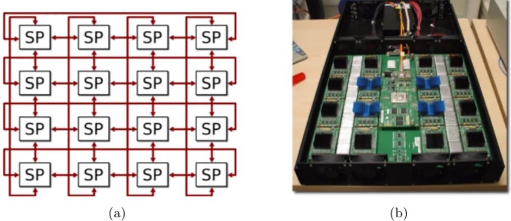
3.8 The Janus computer . . . 57
4 Monte Carlo Simulations and Observables 59 4.1 A few initial words . . . 59
4.2 Observables . . . 60
4.3 Details of the simulations . . . 62
4.4 Thermalization . . . 64
4.4.1 Temperature-temperature time correlation function . . . 65
4.5 The critical temperature and the critical exponents . . . 69
4.6 The ferromagnetic phase . . . 71
5 Results 73 5.1 Overview of known results . . . 73
5.2 A quick reminder . . . 75
5.3 The p = 4 Potts Glass . . . 76
5.4 The p = 5 Potts Glass . . . 78
5.5 The p = 6 Potts Glass . . . 79
5.6 Piercing it all together . . . 82
5.7 The curious case of p = 5, L = 16 . . . 84
6 Conclusion 87
Chapter 1
Overview
The main goal of this thesis is to investigate the critical properties of glassy sys-tems and in particular of the Potts Glass.
It is in general very hard to study this model for a finite size systems, as it usu-ally is for spin glass models, since we have just a few methods to move the exact results we can obtain from Mean Field Theory to finite dimensionality systems (and test their validity): the primary tool available in this case is the simulation, using Monte Carlo techniques, and its corresponding analysis, which is largely based on the Finite Size Scaling ansazt. In Mean Field Theory the Potts Glass exhibits a transition from a paramagnetic to a spin glass phase: the nature and the temperature of this transition depends on the number of states available for spin degree of freedom, p. For p > 4 this transition is expected to be discontinu-ous but without latent heat. There are basically no results known, except for a few ones which are not analytical, for finite dimensional systems, on whether this change in the nature in the transition holds or not, and if the transition happens at all, for different values of p. The aim of this thesis is to fill, at least in part, this gap, by studying the Potts Glass in three dimensions with p = 4, 5, 6. As may appear evident in reading the thesis results are not incredibly precise and are not many: the simulation of these kind of systems is exceptionally hard not only from the physics’ point of view, but also computationally. We were extremely lucky to be able to use the Janus computer to support us in the com-putation, otherwise we would not have been able to complete it. Nonetheless, the total timespan of the simulation campaign was a little more a year and a half. What we were able to obtain is a clear indication of the nature of the phase tran-sitions under study and the critical temperatures at which they happen, together with the confirmation of an empirical equation on the temperature at which ex-pect the spin glass transition given the number of available states, p. Moreover we were able to exclude the existence of a ferromagnetic phase, at least for the range of temperatures (which are L and p specific) we probed in our simulations: this confirms that we are looking at spin glass transition and that there are not “interferences” effects between ferromagnetic and spin glass ordering in the phase
and at the transition we are characterizing.
The results we obtain by all means are to be intended more like a roadmap for successive works on the Potts Glass: they seem to suggest that there could be a change in the nature of the transition for some value of p higher than the ones taken in consideration in this thesis. From the behaviour of Parallel Tempering, and considering also the evolution of the critical exponents as a function of p, there is also the possibility that the change in the nature of the transition happens for the values we are considering: it may be that the small sizes of the system we are able to simulate are rounding the first order transition and make it look like a continuous one. However, this is just a hint: the simulation of systems with larger sizes could resolve doubts on the matter. In this sense this work is more a start of future research than its end.
This is a theoretical thesis, based on theoretical models which describe complex systems. The model is parametric in p, which is more or less like having more models in one: for instance the p = 4 pure Potts Model has been used in the modeling of, in two dimensions, adsorption of N2 on Kr in graphite layers. In
three dimensions it describes the behaviour of FCC antiferromagnetic materials, such as NdSb, NdAs and CeAs, in a magnetic field oriented toward the (1, 1, 1) direction. Its disordered counterpart, the Potts Glass, is used in the study of ori-entational glasses (examples are fullurene, N2− Ar and CuCN). The Potts Glass
shares many connections with other spin glass models, also due to the richness of behaviours given by p, such as the REM model and the p-spin model.
Our preliminary finding that the critical exponents of the phase transition change as p grows, even if the transition still is continuous, can be seen as an enrichment of the phenomenology associated with the model. From this point of view under-standing the behaviour and critical properties for a large interval of p values is both important from the theoretical side and for the possible future applications of the model. This thesis works in this direction: producing results associated to the range of p form 4 to 6. Plans to go to even larger values of p have been stopped by unmanageable complexity of the simulation associated to an ever increasing thermalization time. We see this work as an important step into extracting the complete wealth of information available from Potts models.
The thesis is organized as follows: in the first chapter we will quickly review many concept related to spin glasses, starting from the Ising model and ending with Parisi theory and the Mean Field description of the Potts Glass. The purpose of this chapter is familiarize the reader with the main concepts of Spin Glass theory, in particular (non-trivial) broken ergodicity, frustration, the Parisi order parameter and, in general, the Mean Field Theory of spin glasses. We start from the Ising Model so that even the reader not familiar with the subject can get his bearings.
Chapter two is a (very) quick review of Monte Carlo methods: it cointains the main concepts of Monte Carlo methods, such as importance sampling and the Metropolis and Heat Bath algorithms. It presents also Parallel Tempering, that
3
we have been using extensively in simulations.
Chapter three describes the simulations that we ran on the Potts Glass: all the parameters are described in detail and all the methods, such as the Quotient Method, are explained.
Chapter four contains a description the analysis and of the results we obtained in regard to the critical temperatures and the critical exponents. It also contains a section in which we put together all the information we have been gaining from the simulations to form a coherent picture.
Chapter 2
Introduction
Ferromagnetism is an interesting and fascinating subject in Condensed Matter Physics: a finite fraction of the magnetic moments of materials such as Fe or Ni spontaneously acquire a polarization (at a low enough temperature) and give rise to a macroscopic magnetization.
A simple model to describe the behaviour of this magnetic moments is the Ising model. In this chapter we will start from the Ising model to understand spin glasses.
2.1
A few initial pointers
Before analyzing some of the models that describe ferromagnetism, we shall de-vote a few moments to introduce a few of the most important tools to be used in the description of these models. While this is not by any means a complete approach to the subject, it’s probably best to point them out here. A more complete discussion about models and observables can be found in [1] and [2].
2.1.1 The order parameter
When dealing with phase transitions, as we will, it is of paramount importance to understand and use currently a quantity called order parameter. This is a quantity which is defined to be 0 in one of the phases and to have some other value (non zero) in the other phase. There is no clear indication on which order parameter is better for a certain system, even thought quite often there is a close connection between the chosen order parameter and the symmetries of the Hamiltonian. For example: if we deal with magnetic dipoles, as in the case of the models discussed in this chapter, a clear example of a quantity that goes from zero to some value while the phase changes is the magnetization, which we will define formally in a moment. This quantity is linked to the symmetry of the Hamiltonian: if for example we describe the magnetic moment as a vector (of a dipole moment), the Hamiltonian has spherical symmetry and so is invariant
under a global rotation. In the non-magnetized phase each dipole is free to point anywhere, and so there is no preferred direction, the average of the spins is null. Once we reach the low temperature magnetized phase, then this is suddenly not true, and the spins prefer to point to one of the directions available: suddenly the magnetization reaches a non null value. In this case we have lost some of the initial “symmetry”, this is often called a natural symmetry breaking. While continuing the example it is worth noting that initially, in the high temperature phase, the Hamiltonian had a O(3) symmetry, while in the low temperature phase the symmetry is restricted to an O(2) symmetry (rotations around the vector which is the one “preferred”).
The notion that a system can find itself in states which break the symmetry of the Hamiltonian is very profound: it means that the ergodic hypothesis (that once it has reached equilibrium the system should be found in some configuration proportionally to the Gibbs probability ∝ e−βE) is violated. If, for example, we think of a ferromagnet with all its spins aligned in the “up” direction, it will never be found in the configuration in which all the spins point “down”, in the limit N → ∞ of course, and its motion is restricted to the part of the phase space in which the magnetization is positive. This situation we call broken ergodicity. It is important to stress that, strictly speaking, broken ergodicity and broken symmetry can only occur in infinite systems. In a finite system the entire configurations space is accessible: a finite ferromagnet in a configuration with “up” spins will eventually fluctuate over to a configuration with “down” spins (and then back again, many times) for any non zero temperature.
2.1.2 The correlations
A lot of information about phase transitions comes from diffusion experiments in which one send particles (photons, electrons or neutrons, for example) and then studies the diffusion to which they are subject. For the theory, and the simulation too, the correlation length and the correlation function play a pivotal role. In the phase transition of liquid mixtures one observes an opalescence, Einstein and Smoluchowski explained that are linked to the fluctuations of density and hence of the refraction index, due to an anomalous diffusion of light: we are basically probing the system with photons. In magnetic system one prefers to use neutrons since they tend to be more penetrating and to be able to avoid, at least on first approximation, multiple scatterings.
This scattering involves in this case the two-point correlation function of spins, which is defined as:
G(2)(⃗i,⃗j) = ⟨⃗σi· ⃗σj⟩, (2.1)
where ⟨ ⟩ is a thermal average.
Since in most of the cases our systems are invariant for translation, this quantity really depends only on the difference ⃗i − ⃗j, and, if we can also assume isotropy, only on the distance r = |⃗i − ⃗j|, which is like saying that G(2)(⃗i,⃗j) = G(2)(r). Obviously no real lattice is completely isotropic and invariant for translations,
2.1. A few initial pointers 7
but one can assume it is on scales which are big enough compared to the reticular distance, a.
From the definition of G(2)(r) we can see that it measures the relative alignment between two spins at a distance r: since in the ordered phase spins point for the biggest part in the same direction, if we want to study it fluctuations it’s better to subtract, from G(2), its average, defining in this way the connected correlation function
G(2)c (r) = ⟨( ⃗σi− ⃗σ0) · ( ⃗σj− ⃗σ0)⟩ = ⟨ ⃗σi· ⃗σj⟩ − | ⃗σ0|2 (2.2)
where ⃗σ0 is defined as ⃗σ0 = ⟨ ⃗σi⟩. For T > Tcthe average value ⃗σ0 is null, so that
from G(2)c we recover the original G(2).
Nearby spins tend to be correlated: this correlation is, far from the critical point, extended only for some distance ξ, which is called correlation length, this is basi-cally the extension of “blob” of spins who retain the same state. More formally we can define the correlation length as:
G(2)c (r) ≈ e−r/ξ, r ≫, a T ̸= Tc. (2.3)
Around Tc there’s a change of dynamics and the correlation assumes another
behaviour, the one of a power law: G(2)c (r) ≈ 1
r2−d+η, r ≫ a, T = Tc, (2.4)
where we have introduced our first critical exponent, η, also called the anomalous dimension. This power law behaviour indicates that at criticality fluctuations of the order parameter are correlated on all length, and that the correlation length around criticality becomes infinite (at least in second order phase transitions, while in first order ones it remains finite). If we indicate t = (T − Tc)/Tc, around
the transition we can say that
ξ(T ) =
ξ+t−ν, T > Tc,
ξ−(−t−ν), T < Tc,
(2.5)
where ν is the critical exponent of the correlation length. We shall see some more critical exponents later in this chapter.
This two different behaviours can be actually merged in to one by writing G(2)c (r) = 1 rd−2+ηf r ξ (2.6) where f is a scale function which depends only on the adimensional ratio r/ξ which behaves as f (x) ∼ e−x when x if big, while f (0) can be chosen to be 1, to fix the normalization. The dependency of this function from temperature is mediated only by ξ(T ).
2.1.3 Critical dimensions
Even if the real world is three dimensional it is sometimes useful to forget about it, and just consider the dimensions d of the model as one of the many variables of the system. In fact, there are some cases in which the systems which we try to model present, even in the three dimensional world, a two or even one dimen-sional behaviour: for example graphite’s layers just barely interact, so to render the system, effectively, bidimensional. In another way, there could be a variation of the nature of the dimensional behaviour of the system depending on some parameter: an example of this could be a three dimensional system of magnetic dipoles in which different planes interact with couplings Jz ≪ J , where J are the
couplings between spins on the same plane. At high temperature, where the cor-relation length ξ(T ) is small, interaction between different planes is small, due to the definition of the coupling. But when the temperature is lowered ξ increases, with the effect that big areas of the plane is constituted of spins in the same state, which behave as a unique big magnetic dipole: in this case, even if Jz is
small, the interaction between planes becomes relevant, changing the behaviour of the system from two to three dimensional.
Albeit these examples, there is at least another reason to consider the dimension-ality of the system, d, as a parameter. The existence of a phase transition for a given Hamiltonian depends on the dimensionality of the system: in fact if we lower the number of dimensions in which the system lives, fluctuations become increasingly pronounced, destroying order and thus lowering the critical temper-ature, until eventually there is no longer a transition. Any given model, then, selects a lower critical dimension, dl, such that for d < dl there is no phase
tran-sition for any T . In general one finds that for discrete symmetry models dl= 1,
while for models with continuous symmetry one has dl = 2. Together with the
lower an higher critical dimension ds exists: critical exponents depend on the
dimensionality of the system, too. When d > ds, then the critical exponents are
the same as the ones one can extract from the mean field theory treatment, which we will discuss briefly, of the system itself. The interval of values dl < d < ds
is the most interesting, and also the one where statistical fluctuations play a fundamental role.
2.2
The Ising and Potts models
2.2.1 The Ising model
The Ising model describes variables (which are the modelization of the magnetic dipoles we are dealing with in a ferromagnet), called spins, which sit on a regular d-dimensional lattice. Spins interact only with nearest neighbours, via coupling constants J , which can be positive (for a ferromagnet) or negative (antiferromag-net). Spins can have one of the two values ±1, describing the magnetic moment pointing up or down respect to some axis, on which we take the projection. We
2.2. The Ising and Potts models 9
can then write the Hamiltonian as: H = −J ⟨i,j⟩ σiσj + h i .σi (2.7)
The system can interact also with a constant external magnetic field, h. The notation ⟨i, j⟩ express the sum only over nearest neighbour: in another way we could have written the sum over i < j and used the couplings as Jij in which Jij
was non null only if the spins were nearest neighbours and null otherwise. The magnetization of the system is calculated as:
m = 1 N i σi . (2.8)
If we consider the model in d ≥ 2 and null field, while the temperature is high enough, spins are randomly oriented either up or down, and the net magnetization of the system, in the thermodynamic limit, is null. Lowering the temperature, all of the spins tend to orient themselves in one of the two available directions, thus creating a spontaneous net magnetization for the whole system.
|ms(T < Tc, h = 0)| > 0. (2.9)
We are then in the presence of a phase transition (which is absent if d = 1) from a paramagnetic to a ferromagnetic phase. This transition happens at a temperature Tc.
For h = 0 we are in the presence of a twofold degeneracy, since both states in which all the spins are aligned in one of the two available directions are possible. To remove this degeneracy we can apply a small field to the system and then let the field go to zero, finding, for T < Tc:
ms= lim
h→0m(T, h), (2.10)
which will be positive if we used a field pointing in the “up” direction, or negative otherwise. This comes from the fact that the Hamiltonian is invariant for global inversion of the sign: σi → −σi.
The Ising model can be exactly solved for d = 1 and d = 2. In the latter the solution is quite lengthy and can be found on textbooks of Statistical Mechanics such as the already cited [1] and [2], so we won’t cover it here. For d = 3 there is no known exact solution.
2.2.2 Mean Field Theory for the Ising model
Each spin in the Ising model interacts with both the external field and the field generated by neighbouring spins. The latter is obviously a dynamical variable of the system, which cannot be controlled externally, which fluctuates depending on
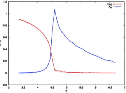
Figure 2.1: Magnetization (in red) for the three dimensional Ising model, from a Monte Carlo simulation of L = 64, using Parallel Tempering for 40 temperatures around the critical value, Tc ≈ 4.51. In green a sketch of the magnetic susceptibility, rescaled to fit
the graph, and hence completely out of scale.
the configurations that the system takes. The idea of the mean field approxima-tion is to replace this interacapproxima-tion between neighbouring spins with the average of the field of all the spins of the system, except the one we are “looking at”. In doing so we will let the spin interact, in some sense, with all the spins of the system, or, if we want to look at the thermodynamical limit, we are dealing with a d = ∞ system.
Even if this limit may appear very distant from the reality of the system we are trying to write a model for, we will see that some of the most essential features of magnets will be described in a quite accurate manner. This approximation was first tried by Braggs and Williams, so it’s known by their names.
Let’s now consider an Ising model defined on a d-dimensional lattice, with the same Hamiltonian as before:
H = −J 2 ⟨i,j⟩ σiσj − h i σi, (2.11)
where we consider each distinct pair i, j once. We define, again, the magnetization as: m = 1 N N i σi , (2.12)
2.2. The Ising and Potts models 11
where by ⟨⟩ we express the thermal average. We can write the product σiσj as:
σiσj = (σi− m + m)(σj− m + m)
= m2+ m(σi− m) + m(σj− m) + (σi− m)(σj − m), (2.13)
where taking the thermal average of the last term basically measures the fluc-tuations of the spins. The mean field approximation basically consists in the “forgetting” of this last term, writing the Hamiltonian as:
H = −J 2 ⟨i,j⟩ σiσj− h i σi ≈ − J 2 ⟨i,j⟩ −m2+ m(σ i+ σj) − h i σi. (2.14)
If now we call z the coordination number of the lattice (the number of the nearest neighbour spins, z = 2d) we can now rewrite the first term in the sum over ⟨i, j⟩ as: −J 2 ⟨i,j⟩ −m2= 1 2 i J zm2= 1 2J zN m 2, (2.15)
while the second term in the same sum can be rewritten as: −J 2 = ⟨i,j⟩ (σi+ σj) = −J zm i σi. (2.16)
So now we can rewrite the whole Hamiltonian as: HM F = 1
2N J zm
2− (J zm + h)
i
σi. (2.17)
In this view all spins are decoupled, and hence we can calculate the partition function as: ZNM F = {σ} e−βHM F = e−12βJ zm2 σ=±1e(βJ zm+βh) σN = e−12βJ zm2[2 cosh (2 βJ m + βh)]N. (2.18)
The free energy per spin will be then: fM F(T, h) = − 1 βN ln Z M F N = 1 2J zm 2− 1 β ln [2 cosh (βJ m + βh)] . (2.19) Now, given that the magnetization is the derivative of f in respect to the field h, this satisfies the self-consistent relation:
m = −∂f
∂h = tanh (βJ zm + βh) (2.20) If now we want to study the appearance of magnetized phases, we have to study the transcendent equation:
which can be easily done in a graphic way: in fact we can plot the hyperbolic tangent and the line y = m and look for intersection points. The point m = 0 is always a solution. If the derivative of tanh (βJ m) in the origin is bigger than 1 (or, equivalently, if βJ > 1), then there are two more solutions, of opposite signs but with the same modulus, ±m0. So for βJ z = 1, and hence the temperature
is Tc= J z/k, we have a phase transition from a disordered to an ordered phase.
Spins are aligned to the field, if we had a field which we will let it go to 0: if we have h → 0+, then the magnetization will be m = m0, otherwise if h → 0−,
m = −m0.
In the case of a non null expected value of the magnetization the symmetry Z2
is spontaneously broken. In the ordered phase, the remnant of this symmetry is that we can change one solution in the other, m0 → −m0 and viceversa.
2.2.3 The critical exponents of the Ising model
Using Mean Field Theory we can calculate the critical exponents for the Ising model. Let’s write
t = T − Tc Tc
(2.22) and rewrite the autoconsistent relation as:
m = − h kTc
+ (1 + t) arctanh m. (2.23) Let’s start with the case of h = 0: in this case, for T ≈ Tc, t ≈ 0, the value of
the magnetization is small, so that we can expand in series the right hand side of the last equation, obtaining:
m0 = (1 + t) arctanh m = (1 + t) m0+ 1 3m 3 0+ 1 5m 5 0+ . . . . (2.24) If we now invert this to obtain m0, we get:
m0 = (−3t)
1
2 [1 + O(t)] . (2.25)
So, the critical exponent β has a value of 12, since this critical exponent is the one that “regulates” the behaviour of m near the critical temperature in absence of an external field:
m = m0(−t)β, (2.26)
while in presence of an external field the system behaves as: M(h, Tc) = M0h
1
δ. (2.27)
The critical exponent γ is related to the magnetic susceptibility χ as: χ(h = 0, T ) =
χ+t−γ, T > Tc,
χ−(−t)−γ, T < Tc.
2.2. The Ising and Potts models 13
Since χ = ∂m0/∂h, we differentiate the equation 2.24 to obtain:
χ = − 1 kTc + (1 + t) 1 1 + m2 χ. (2.29)
Now, for h = 0 and T > Tcwe have m0= 0, so that χ satisfies se equation
χ = − 1 kTc + (1 + t) χ, (2.30) which results in χ = 1 kTc t−1. (2.31)
On the other hand, if we have h = 0 and T < Tc, we have:
χ = 1 2kTc
(−t)−1, (2.32)
so that we can conclude that the critical exponent γ = 1.
To calculate the critical exponent δ, we consider equation 2.24 again, expanding the hyperbolic function and simplifying we obtain:
h kTc ≈ 1 3m 3+ O(m5) (2.33) or m ≈ h13 (2.34) yielding δ = 3.
Mean field treatment of the Ising model in d-dimensions has let us understand the behaviour of the model around the phase transition, and have a rough value of the critical exponents, which we resume in the table 2.1: the values are approximate, and will not yield true for systems at a specific dimensionality.
Exponent Value in MFT Specific Heat, C α 0 Order parameter, m(T ) β 1/2 Susceptibility, χ γ 1 m(h) δ 3 Correlation Length, ξ ν 1/2 Anomalous Dimension η 0
2.2.4 The Potts model
The Potts model is a generalization of the Ising model: aside its theoretical importance, it is very useful when describing spins which cannot be assimilated to a 2-states system and more freedom is needed.
To do this, the Potts model prescribes, for each spin, p available states, instead of just the two of the Ising model. Also, as we can see in the Hamiltonian
H = −J
⟨i,j⟩
δ(σi, σj) (2.35)
the interaction is different: it takes place only when the spins σi and σj are in
the same state, in which case the contribution to the energy of the system is −J . Whereas the Ising model was invariant under global spin inversion σi→ −σi, the
Potts model is invariant under the group Sp of permutations of p variables, which
is a non abelian group if p ≥ 3. In the Potts model we regard the “states” of the spins as label, which are in this sense inessential, and could be anything: any set of numbers or colors or whatever else.
In the case p = 2, if we take ±1 as the values of the spins, using the identity δ(σi, σj) = 1/2(1 + σiσj), we can see that, excluding a multiplicative constant,
the Potts model is equivalent to the Ising model we just discussed. The partition function of the Potts model for a lattice of N spins is :
ZN = {σ} K ⟨i,j⟩ δ(σi, σj) , (2.36)
where we have written K = βJ = J/kT .
2.2.5 Mean Field Theory for the Potts model
We analyze the mean field theory for the Potts model, as we did for the Ising model. We shall see that the behaviour of this model is richer, in a sense, than in the Ising case: the nature of the phase transition changes depending on p. As said before in mean field theory each spin in the lattice interacts will all the other N − 1 spins, so that we can write the Hamiltonian as
HM F = 1 NJ z
i<j
δ(σi, σj) (2.37)
where we have introduced for convenience a factor 1/N and z, as before, is the coordination number of the lattice.
To solve the model we will proceed in calculating the free energy, F [{σ}] = U [{σ}]−T S[{σ}] as a function of configuration {σ} and the look for its minimum. This approach is simplified by the fact that, even if to specify a configuration we have to indicate the state of each of the N spins, this function is degenerate,
2.2. The Ising and Potts models 15
since it can assume the same value for different configurations of the system: it is then useful to introduce variables which will make this propriety obvious. To do this we introduce, given a configuration {σ} of the spins, xi = Ni/N the number
of spins which are, for that configuration, in the state i, with i = 1, 2, . . . , p. Obviously we need to impose
p
i=1
xi = 1. (2.38)
Since there are 2 N 1
1(Ni−1) coupling of type i in the Hamiltonian, the energy U [{σ}]
of this configuration is given by: U [{σ}] = − 1 2NJ z p i=1 Ni(Ni− 1). (2.39)
Dividing now by the number of spins and considering the thermodynamic limit, N → ∞, we obtain: U [{σ}] N ≈ − 1 2J z p i=1 x2i. (2.40)
Since there are
N !
N1! N2! N3! . . . Np!
(2.41) way of dividing the spins without an energy change, we have an entropy
S[{σ}] = k log N ! N1! N2! N3! . . . Np! . (2.42)
Using the Stirling approximation (log z! ≈ z log z, if z ≫ 1) for each term, and using the definition of xi we can write:
S[{σ}] N ≈ −k p i=1 xilog xi. (2.43)
So that we can finally write the expression for the free energy per spin: F (xi) N = f (xi) = − p i=1 Jz 2 x 2 i − kxilog xi , (2.44)
which we will minimize. We have also to keep in mind the condition expressed in (2.38): it will be automatically satisfied if we parametrize the xi as [3]
x1 = 1p[1 + (p − 1)s]
xi = 1p(1 − s) , i = 2, 3, . . . , p (2.45)
with 0 ≤ s ≤ 1. If we assume J > 0 (the ferromagnetic case), this parametrization is mindful of the possible breaking of the symmetry of the group of permutations
Sp when we are in the phase of low temperatures. Substituting this expression
for the xi in the energy and in the entropy leads us to β N [F (s) − F (0)] = = p − 1 2p Kzs 2−1 + (p − 1)s p log[1 + (p − 1)s] − p − 1 p (1 − s) log(1 − s) ≈ −p − 1 2p (p − Kz)s 2+ 1 6(p − 1)(p − 2)s 3+ . . . (2.46)
From this we can see that the cubic term of the free energy changes sign when p = 2. Let’s consider the two cases in separate ways.
For p < 2, the minimum condition for the free energy is expressed by Kzs = log 1 + (p − 1)s
1 − s
. (2.47)
s = 0 is always a solution for this equation, but for Kz > q where q is the deriva-tive of the right hand side of 2.47, we have another solution for s ̸= 0. The two solutions coincide for J β = K = Kc = q/z, which is the critical point related
to the transition for p ≤ 2. In this case we have a continuous (or second order) transition.
For p > 2, the situation is different, since changing K, there is a critical value for which the free energy exhibits a discontinuous jump from s = 0 to s = sc.
This discontinuity is a characteristic of first order phase transitions (or discon-tinuous).In this case the critical values for Kc and sc are obtained by solving
simultaneously F′(s) = 0 and F (s) = F (0): zKc = 2(p − 1) p − 2 log(p − 1), sc = p − 2 p − 1. (2.48)
Calculating the internal energy of the system, U = −J zp − 1
2p s
2
min (2.49)
we see that for K = Kc there’s a jump in the function, corresponding to a value
of the latent heat L per spin
L = J z (p − 2)
2
2p(p − 1). (2.50)
2.3
Spin Glasses
Spin glasses are magnetic systems in which the interactions between magnetic moments are “in conflict” due to some quenched, or frozen in, structural dis-order. This mean, among other things, that no conventional long range order
2.3. Spin Glasses 17
(ferromagnetic or antiferromagnetic) can be established. Nevertheless, these sys-tems exhibit a transition into a phase in which spins are aligned with this random order. On the other hand these “conflicts” result in the other characteristic of spin glasses: frustration. Namely, we say a spin is in a frustrated state when, whichever state it is in, it cannot reach the lowest energy state, and so “agree” (where the meaning of “agree” depends on the sign of the coupling between the spin and the neighbours) with all its neighbours.
These two key elements, disorder and frustration, seem to suggest that the spin glass phase is intrinsically different from the forms of order we have been dealing until now, such as ferro or antiferromagnetic, and so new tools and concepts are needed to describe it. Experimentally it is not hard to find systems which behave as spin glasses, quite the contrary.
As it was the case with ferromagnets, we will employ models which will, hope-fully, be simple enough to be used both theoretically and in simulation and still incorporate the necessary disorder and competing interactions that lead to frus-tration.
While we will consider spin glasses only of magnetic nature, which is to say that the “spin” degree of freedom is magnetic, it has been a while since people started to find spin glasses phases in different fields: properties analogous properties have been seen in ferroelectric-antiferroelectric mixtures (in which case the elec-tric dipole moment takes the place of the magnetic dipole moment), in amorphous alloys and magnetic insulators (where the distances between magnetic moments is entirely different from that of the crystalline magnetic systems) and in disor-dered molecular crystals (where the electric quadrupole moment plays the role of the spin) in which a kind of orientational freezing has been observed.
Moreover a behaviour similar to the one of spin glasses has been observed not only in Physics: developments resulting from the study of spin glasses have found application in Computer Science, Biology and Mathematics.
A possible example of spin glass, which is well known, are alloys in the form EuxSr1−xS. In the Eu-rich limit, this is a ferromagnet with ferromagnetic nearest
neighbours and antiferromagnetic next-nearest neighbours interactions. The Sr is magnetically dead, so a substitution of Sr for Eu just dilutes Eu. We can write the Hamiltonian as H = −1 2 i,j Jijcicj⃗σi· ⃗σj, (2.51)
where ci is 1 or 0 with probabilities x and 1 − x. This model has competing
interaction, which, hopefully, will lead to frustration.
2.3.1 The Edwards-Anderson (EA) model
Starting form the Hamiltonian 2.51 we can simplify, if it turns out to be theo-retically more convenient. The following Hamiltonian has been written first by
Edwards and Anderson in 1975 [5], in the paper that marks the start of spin glass Theory as an active area of Theoretical Physics. The model is defined on a translationally invariant regular lattice:
H = −1 2
ij
Jij⃗σi· ⃗σj, (2.52)
where the Jijare taken to be identically distributed independent random variables
with distribution that depends only on the lattice vector separation ⃗ri− ⃗rj. In
particular it’s convenient to consider
P (Jij) = 1 2π∆ij exp − J 2 ij 2∆ij , (2.53)
a symmetric Gaussian distribution, or
P (Jij) =
1
2δ(Jij−∆ij) + 1
2δ(Jij +∆ij), (2.54) a double delta function. In either case, the model is specified by
[Jij2]av≡ ∆ij ≡ ∆(⃗ri− ⃗rj), (2.55)
where we have introduced the average [ ]av as the average of the distribution of
the random variables.
This model, in both the double delta and the Gaussian version, clearly has both the randomness and competing interactions we were looking for, but it turns out we can proceed to some further simplifications:
• instead of Heisenberg-like spins, ⃗σi we may consider Ising-like spins with a
single component, σiz ≡ σi
• we can consider the interactions between spins to fall off very quickly, re-sulting in only nearest neighbours or next-nearest neighbours interactions • we can “forget” to deal with a lattice, and just have spins interacting with
a finite number of spins, which can be anywhere in the system
and still be able to obtain the spin glass phase. It’s desirable that, even with any simplification, there should not be significant differences in the behaviour between models, given that all their forces fall off in the distance in the same way (eg. they are all nearest neighbours) and that the nature of the spins is the same (eg. we are dealing with Ising spins or Heisenberg spins).
2.4. How do we deal with disorder? 19
2.4
How do we deal with disorder?
In the definition of the Hamiltonian of the EA model, we have introduced random-ness, which in turn introduces special features in Statistical Mechanics. Basically we don’t know all the parameters of the Hamiltonian we are trying to study, but only their distribution, for example of the Jij or random fields hi, so that we
don’t have a particular realization. We can, for example in simulation, simulate different distribution realizations, and then average over them, which corresponds to the [ ]av average, but this is closer to experiments than to theory.
Also, we could calculate the quantities of interest for a given realization of the Jij, but this is not what interests us: we want to calculate these quantities for
the given distribution of these parameters.
Fortunately Statistical Mechanics comes in our help with the averaging in the limit of large systems. Just as it was the case with the ferromagnetic models, and in general, we know that the fluctuations of the energy of the system around the thermal average are of order N−1/2, so we expect that the sample-to-sample fluctuations will go to zero in the limit of a large system. A quantity which ex-hibits this property is said the be self-averaging. If we know that the quantity that is of interest to us has this property, then we can expect different experi-ments to yield the same result, and even more interestingly, that the theoretical calculation in which we average over disorder agrees with the experiments. But there are some quantities which are not self averaging, for example the local inter-nal field of a spin i which depends sensitively from the local environment. Most of the quantities which we want to measure are sums or integrals over the entire volume of the sample (so that we call them “extensive” quantities) and statistical fluctuations will become small for large systems.
We have thus two different kind of average to calculate: the first is the usual ther-mal average, which in principle is carried out in each sample, and the average over the disordered random parameters. As is often the case, the average that we want to calculate can be expressed as, or in terms of derivatives of, the free energy with respect to auxiliary fields. We then start with the partition function, which is the trace over the thermodynamic variables and function of the fixed interaction strengths for that sample:
F [J ] = −T ln Z[J ]. (2.56) Now, F [J ] is an extensive variable, so we can think of it as self-averaging, and so the experimentally relevant quantity is
F ≡ [F [J ]]av≡
dP [J ] F [J ] = −T
dP [J ] ln Z[J ]. (2.57) It’s important to note that it’s ln Z which should be averaged, and not Z itself: the reason is that Z is not an extensive quantity, and so self-averaging cannot be expected to apply to it, and so [Z]av is not a physically relevant quantity.
As an obvious extension of this argument one can calculate the magnetization in a macroscopic sample as
[M ]av= T
∂[ln Z[J, h]]av
∂h (2.58)
and in a similar fashion for other extensive quantities. For correlation functions we need to extend this definition (albeit just formally) to site-dependency:
[⟨σiσi⟩ − ⟨σi⟩⟨σj⟩]av= T2
ln Z[J, h]]av
∂hi∂hj
. (2.59)
How do we evaluate these averages? One way is to write down the formal expres-sion for F [J ] or its derivative (for example obtained with perturbation theory) and average them, term by term, over the distribution of the Jij. This procedure
works, and it’s practical. But it is also often very useful to be able to carry out the averaging formally from the beginning: this will leave us with a problem in which the disorder no longer appears explicitly. If the system is translationally invariant, we would end up with a nonrandom, translationally invariant Statisti-cal Mechanics problem, which we would then be able to solve.
Since we want to average ln Z we cannot just write the integral in 2.57 as if we were dealing with Z: we basically want to “fix” the Jij as quenched variables, and
then let the spins σi just adapt to the couplings. If we were to write something
like [Z[J ]]av= Tr σ ⟨i,j⟩ dJij 2π∆ij exp − J 2 ij 2∆ij + βJijσiσj , (2.60)
which can be solved by completing the square, we would be dealing, then, with the wrong Physics: we are in fact writing a nonrandom system in which both the spins and the coupling Jij are thermodynamical variables, which are traced
on the same footing. In the systems we will be dealing with, if we look at it from an experimental point of view, the Jij are frozen in to their configuration
when we prepare the sample to analyze by rapid cooling or, as we just mentioned, quenching. In this sense we may call the kind of average we want to do “quenched average”.
2.4.1 The Replica Trick
We cannot write the integral as in 2.60, because we want to average over ln Z and not Z, since the free energy F = −kT ln Z: we have a “trick”, quite common in Statistical Mechanics of random systems, to deal with the complexity from that arising. It is called the replica method and it’s based on the identity
ln Z = lim
n→0
Zn− 1
2.5. Broken Ergodicity, the Spin Glass phase and order parameters 21
and the fact that the average of [Zn]av can be carried out almost as simply as
[Z]av if n is an integer. We write Znas Zn[J ] = Tr {σ1},{σ2},...,{σN}exp −β n α=1 H[σα, J ] . (2.62)
We say then that we have replicated the system n times, and hence the termino-logy “replica method”. The index α which appear in 2.62 identifies the replica and is called replica index. For the EA model, with Ising spins, the average of 2.62 over the Gaussian couplings is then
[Zn]av = Tr{σ1},{σ2},...,{σn}exp 1 4β 2 ij ∆ij αβ σαiσβiσjασβj ≡ Tr{σ}exp (−βHeff) (2.63)
which is basically like converting the disordered problem into a non-random one, involving four-spins interactions. For a general distribution of the Jij we can
write: β Heff= − 1 2 ij ∞ p=1 1 p![J p] c(β n α=1 σiασjα)p, (2.64) where [Jp]cis the p-th cumulant of the distribution of the Jij. After solving these
effective problems in any way we can, we have to take the limit n → 0 of the result.
The cumulants (here we report just the first two): [J ]c = [Jij]av= J ,
[J ]c = [Jij2]av− [Jij]2av≡ (∆Jij)2 (2.65)
in terms with p > 1 introduce interactions, as to say: couplings, between different replicas of the disordered system.
2.5
Broken Ergodicity, the Spin Glass phase and
or-der parameters
Since we don’t know qualitatively how the spin glass phase is, we can’t be sure that the order parameter we have defined for the ferromagnetic phase is still a good choice. In this section we will try to understand better what changes in the new phase, and it will turn out that we need a new order parameter.
In an Ising ferromagnet we do have broken ergodicity when we are dealing with an infinite system and a temperature that is below the transition temperature: as we said already, in this case the configuration space is basically divided in two (for two are the directions possible for the magnetization) and there is no way for
a system magnetized in one direction to go spontaneously into the region of the configuration space where the magnetization is in other direction. This has an-other very important consequence: when we write some quantity that is defined by a thermal average we have to be careful about what we mean. If we were to mean it as a conventional Gibbs average over all the spins configurations with the symmetric weight exp(−βH[{σ}]) then it would vanish by symmetry. Instead we restrict our averages over part of the configuration space: for example if in the ferromagnetic phase we restrict ourselves to one of the two halves just mentioned then the magnetizations would differ by sign, resulting in the two well known values of it. In this sense the broken ergodicity has to be put in “by hand” by restricting the trace we use to define the thermal averages to configurations near the chosen phase. In a ferromagnet we could restrict ourselves simply by applying a small field to the system (in the Hamiltonian) and then letting it go to zero once we have taken the thermodynamic limit. In this case it is crucial the order in which we take the limits: were we to take them in the opposite order (first h → 0 and then N → ∞) this would not, obviously, work. In another way, we could introduce the restriction over the trace by means of boundary conditions: if we want to end in the “up-spin” phase, we can set the spins on the boundary of the system to be fixed “up”.
Another useful way to describe broken ergodicity is to interpret expectation val-ues for quantities like ⟨σi⟩ as averages over time intervals [0, t] taking the limit
t → ∞, noting that if there’s broken ergodicity these long-time averages will not vanish.
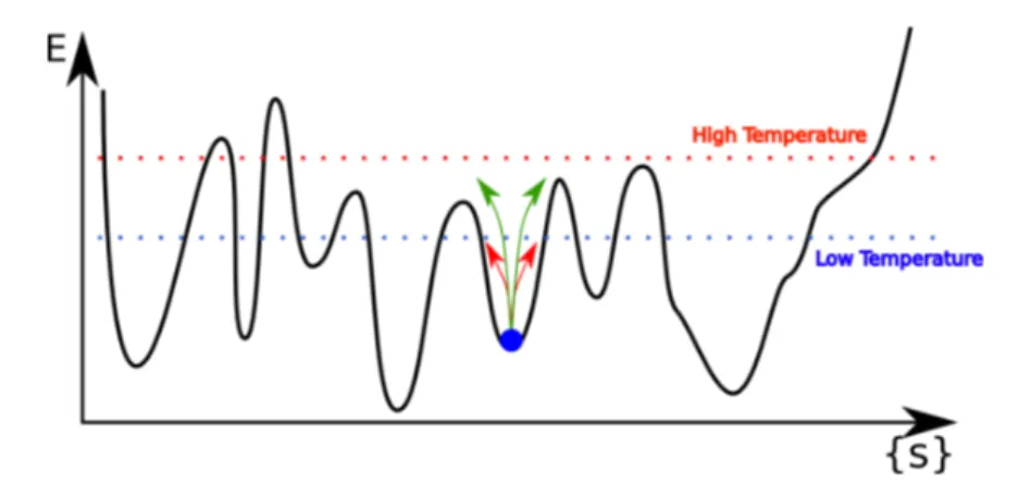
In a spin glass we could suppose, as we did for the ferromagnet, to find two stable states related by an overall spin flip symmetry, but it turns out not to be the case: we have to take in account the possibility, given randomness and competing interactions, to find a non trivial broken ergodicity: in another way, we have to take into account the possibility to find many stable states. We could visualize the situation as a landscape where for each configuration we calculate the free energy F : in a ferromagnet there are just two states minimizing F below the transition. Under a temperature Tf, there will be many states that do the
same for the spin glass: these minima will be the bottom of valleys of the energy separated by barriers which, in the limit N → ∞ will become infinitely high, rendering impossible to move from valley to valley, thus breaking ergodicity. If we increase the temperature above Tf the valleys will become less deep and then
just disappear, and there will be just one valley with the minimum at m = 0. The configurations {σ} which contribute to the partition function inside a single valley (or phase, let’s call a) all lie in the region of spin configurations space near the minimum (possibly comprising many sub-valleys).
When a system finds itself in one of these valleys it will exhibit the behaviour and the properties which is typical of that valley. In general, they will differ from true equilibrium properties, since these would include averaging over all valleys with appropriate relative thermal weights. If we wish to calculate the properties of the system inside a single valley (which as we said might differ, for example,
2.5. Broken Ergodicity, the Spin Glass phase and order parameters 23
in the magnetization) we have to restrict our trace of the partition function only to the appropriate valley.
Since there many possible stable states, the trick to impose an external field, as we did in the ferromagnetic case, uncorrelated to the single spins magnetizations will not help in tentatively select out only a single phase: in this sense broken ergodicity makes the definition of “thermal averaging”, and the notion of an order parameter for spin glasses, a non trivial task. In fact, different ways to project onto particular phases would lead to different values of the observables: this is also one of the main reasons why it is so difficult to write down a mean field treatment for Spin Glasses.
So far we have been dealing with what happens to a sample, but of course we want our results to be averaged over many samples, or, in another way, to be averaged over the disorder probability. The order parameter of a ferromagnet, the magnetization, even if averaged over the disorder will not do, for the reason outlined above, so we have to look for something else, even if it would clearly van-ish in the limit of null external field: we have to look to some higher moments. If we were to consider the breaking of ergodicity as essentially a dynamical process, we could consider, as Edwards and Anderson did in their paper in 1975, [5], the order parameter as
qEA= lim
t→∞N →∞lim [⟨σi(t0) σi(t0+ t)⟩]av, (2.66)
where the average is over a long (infinitely long) set of reference times t0. This
would be null (in the limit of a vanishing external field) if the system is ergodic, and nonzero if the system is trapped inside a single phase. One must take the N → ∞ limit before the t → ∞ since the correlation will eventually die out, as a function of time, as true equilibrium is reached, for a finite system. Since, instead, an infinite system will never escape the valley it is in, the parameter qEAmeasures
the mean square single-valley local spontaneous magnetization, averaged over all possible valleys. In terms of thermal averages we would write it as
qEA= a Pa(mai)2 (2.67) where Pa= e−βFa ae−βFa , and mai = ⟨σai⟩ (2.68) inside the valley (or phase) a. Assuming (it can be proved in mean field theory, and for single models) that this quantity is self-averaging we can write:
qEA = 1 N a Pa i (mai)2. (2.69)
This qEA is not, of course, the mean square local equilibrium magnetization, for
the reasons outlined above. If we consider
q = [⟨σi⟩2]av= [m2i]av= a Pamai 2 av = ab PaPbmaimbi av (2.70)
this is the equilibrium (or Statistical Mechanics) order parameter, denoted simply by q. Equivalently we can write
q = 1 N i ab PaPbmaimbi av . (2.71)
We can also define q for a single sample qJ = 1 N i m2i = 1 NPaPbm a imbi. (2.72)
We can see, from the definitions, that q differs from qEAby having an inter-valley
term. It is often useful to consider also
∆ = qEA− q (2.73)
(which is semidefinite positive, and zero only if there is just a single phase) which basically measures the degree of broken ergodicity. We can imagine the differences between qEA and q by considering a non infinite system: on a long
enough timescale (that could be very long) the system will, statistically, visit many valleys with their relative thermal weights, so that true equilibrium is reached and inter-valley terms in q contribute. On a shorter time scale there is no time for the system to change valley, so that only qEAis the physically relevant
quantity. Obviously we could imagine a somewhat intermediate picture, in which only a few valleys are “visitable” for the system (and so no true equilibrium is reached): in this case we should consider a quantity between these two limiting cases, q and qEA.
In ferromagnets the susceptibility can be written as χloc= 1 N i χii= β 1 − 1 N i m2i (2.74)
where χii is defined as χii= β ⟨(σi− ⟨σi⟩)2⟩. We can then write, for a system in
a single phase,
χloc= β(1 − qEA). (2.75)
The average local equilibrium susceptibility, obtained with the equilibrium ex-pression mi =aPamai, can be written as
2.5. Broken Ergodicity, the Spin Glass phase and order parameters 25
where is worth noting that χJ is not a self-averaging quantity if there is ergodicity
breaking. While it’s clear that in a macroscopic experiment χ, due to the fact that barriers are infinite, comes only from a single valley, since there is strict ergodicity breaking, if the barriers are not infinite one can hope to observe a crossover from single-valley to equilibrium in χ, from short to long observation times.
Another interesting quantity to look at, once we know we have many valleys, is the “overlap” qab= 1 N i
maimbi, obviously for a single sample, (2.77) when a and b run over the many different phases one can expect to observe values of qab in the range [−1, 1]. Following Parisi ([6], [7], [8] and [9]) is natural then
to define the distribution
PJ(q) ≡ ⟨δ(q − qab)⟩ ≡
ab
PaPbδ(q − qab) (2.78)
and its average over the couplings
P (q) ≡ [PJ(q)]av. (2.79)
For a system with just 2 phases, P (q) is the sum of two deltas, and by introducing an external field, we can just simple it down to a single delta function. If there is strong ergodicity breaking P (q) may have a continuous part, indicating there is, maybe, a continuum of possible overlaps between phases. Hence, by studying P (q) we can tell systems in which we have a “conventional” broken symmetry from those where we have a non-trivial ergodicity breaking. Given the probability distribution we can then rewrite q and qJ as:
q = 1 −1 P (q)q dq, and qJ = 1 −1 PJ(q)q dq. (2.80)
If we let the system be without an external field P (q) is symmetric: it is in fact possible to find, for the overlap qab, the corresponding value −qab by simply
reversing all spins in a and b. If instead we apply a small field, then only the states with the magnetization aligned with the field will be selected, and therefore only positive overlaps will enter P (q): the lower limit of the integral is then 0, and q is finite.
Until now we have devoted a lot of attention to different order parameters, even if we have not yet tried to represent them in the replica formalism we have introduced. We begin considering the ferromagnetic order parameter:
M = [mi]av≡ [⟨σi⟩]av= Tr{σ}σie−βH[{σ},J] Z[J ] av , (2.81)
and write n−1 factors of Z[J ] (applying the replica trick) on both numerator and denominator. In the limit n → 0 the denominator goes to 1 so that we need to take the average over disorder only over the numerator. Introducing the replica indexes we find, then
M = Tr {σ1},{σ2},...,{σn} σ α i exp −β n β=1 H[{σβ}, J ] av , (2.82)
where we can carry out the averaging over the disorder as we did for the calcu-lation on [Zn]av, obtaining
M = Tr {σ}σiαexp(−βHeff), (2.83)
which, taking the limit n → 0, can be written as
M = ⟨σiα⟩, (2.84)
where the “thermal” average is taken with the effective Hamiltonian Heff, since
we can use the fact that
Tr{σ}exp(−βHeff) ≡ [Zn]av→ 1. (2.85)
There is one big point that needs to be addressed here: our result should be independent from which replica α is the one chosen for σαi, since all replicas are (supposedly) “created equal”. What if they are not? What if some replicas are “more equal” than the others? If in the solution of our Hamiltonian all the ⟨σαi⟩ turn out to be equal then we have no problems, but what happens if it turns out they are not?
We turn our attention back to the equilibrium spin glass order parameter, finding q = qαβ ≡ ⟨σiασiβ⟩ (2.86) for any replicas α ̸= β, since otherwise we would obtain, for Ising spins, (σiα)2 ≡ 1. Considering the possibility to have a broken replica symmetry, we have to average over all the possible ways to break it
q = lim n→0 1 n(n − 1) α̸=β qαβ. (2.87)
In the same way we can express P (q) as P (q) = lim n→0 1 n − 1 α̸=β δ(q − qαβ). (2.88)
If P (q) is not a delta function but has a more complex structure, the matrix qαβ must depend on α and β in a non trivial way and the replica symmetry is
2.5. Broken Ergodicity, the Spin Glass phase and order parameters 27
broken [18], which in turn signals the existence of many equilibrium states [11]. In another way, we can say that whenever averages depend on the indexes of the replicas they are calculated with, we have broken replica symmetry.
Comparing this to the expression of PJ(q) in equation 2.78 we see that the
distribution of values of the matrix elements qαβ in the replica symmetry breaking case and the distribution of the overlap between different states when there are many states must be the same.
Finally we can identify with qEA the largest value of qαβ in a broken replica
symmetry solution
qEA= max αβ q
αβ. (2.89)
2.5.1 Susceptibilities
A quite important quantity in the study of spin glasses is the Spin Glass Sus-ceptibility, which has the role corresponding to the one of the susceptibility for ferromagnets. This quantity is defined as
χSG( ⃗Rij) = [χ2ij]av= β2[(⟨σiσj⟩ − ⟨σi⟩⟨σj⟩)2]av (2.90)
and its Fourier transform χSG(⃗k), evaluated for ⃗k = 0.
Above the freezing temperature Tf this reduces to χSG= β
2
N
ij⟨σiσj⟩2.
In a ferromagnet the susceptibility is the magnetization induced by an external field on the system per unit of external field, h. In a spin glass we can induce a non-zero q, even above Tf, by introducing random external fields hi. We can
then write
⟨σi⟩ =
j
χijhj (2.91)
and we can, by squaring and averaging over the disorder obtain q =
ij
[χ2ij]avσ2 = χSGσ2 (2.92)
where σ2 is the variance if the random field and where we have assumed that the random fields hi are uncorrelated. We can see that σ2 acts as a conjugate field
for the order parameter q pretty much as the external constant field h did for the magnetization m in the ferromagnet. While above Tf we need hi if we want
have a non zero q, below Tf q is finite even if σ2 → 0, thus, by analogy with
the ferromagnetic case, we expect the susceptibility, χSG to diverge when one
approaches Tf from above: the correlation length of χSG(⃗r) diverges in the same
way as the same quantity of the spin correlation function did in the ferromagnetic case.
One last important point: susceptibility is measurable, through what is called the non-linear susceptibility, which is defined as the coefficient of −h3 in the expansion of the magnetization in powers of the external field:
Figure 2.2: Plaquettes without and with frustrated spins: the spin at the site with the question mark cannot satisfy both its couplings at the same time.
As χ is proportional to the thermal variance ⟨(σ − ⟨σ⟩)2⟩, one finds
χnl= − β3 3 N i σi 4 c (2.94)
where we indicate with the subscript c a cumulant average. Above Tf the
cumu-lant is expressed as i σi 4 c = ijkl ( ⟨σiσjσkσl⟩ − 3 ⟨σiσj⟩ ⟨σkσl⟩ ) = 4N − 6 ij ⟨σiσj⟩2 (2.95) which leads to χnl= β(χSG− 2 3β 2) (2.96)
and thus measurements of χnlgive us important information about the spin glass
transition.
2.6
Frustration
It is safe to indulge in the thought that broken ergodicity is caused by the ran-domness and the frustration, at least the non trivial one, so it’s a good idea to spend some time describing kinds of frustration, and it effects, since we already journeyed, even if only briefly, in the realms of randomness.
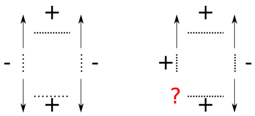
To clarify what we mean by frustration we turn our attention to an Edwards-Anderson model with Ising spins, σ ∈ {±1}, on a square lattice, with couplings coming from a double delta function, so that, fixed J they can only take values from the set {±J }, and with only nearest-neighbours interactions. Instead of considering the whole lattice we focus for a moment only on four spins and their
2.6. Frustration 29
four couplings: this elementary portion of lattice is commonly called a “plaquet-te”. Since the couplings are taken randomly from the distribution there is an equal probability to end up with an odd or an even number of negative bonds. Now, if the number of negative bonds is even, then it is always possible to find an arrangement of the spins (and it’s spin-flipped counterpart) which satisfy all the bonds. All one needs to do is to start at some point fixing a spin and then follow the couplings setting the spins so that the latter are satisfied, which basically means multiplying the spin by the value of the coupling and setting the result as the next spin. If, otherwise, the number of negative couplings is odd, then applying the same simple algorithm for setting the spins (or any other algorithm, for all that matters) will result in a conflict between the value of the spins, at some point. Trying to proceed by going back and flipping a spin previously set so to avoid this conflict will result in the spins at the ends of the other coupling in creating a new conflict. The term “frustration” refers to the inability to satisfy all the bonds simultaneously. The second plaquette in figure 2.2 exhibits frus-tration, and has an extra ground state degeneracy beyond the one that follows from global spin inversion. It is sometimes useful to think about it in terms of bonds variables instead of spins: we can define it as Aij = (σiσj sgn Jij) and, if
a bond is not satisfied, we see that Aij = −1. Changing a spins, in a frustrated
plaquette, moves the unsatisfied bond to the neighbouring bond.
2.6.1 Trivial and nontrivial disorder
A simple example, following Mattis [13], is helpful in describing what is meant by trivial and nontrivial disorder: not all kinds of disorder gives rise to frustration, and hence to spin glass behaviour. Let the bonds be
Jij = Hξiξj, (2.97)
where the ξi are independent and take on the values ±1 with equal probabilities.
Half of the bond are indeed positive and half negative: this is what happens in competing ferromagnetic and antiferromagnetic interactions. But the Jij are not
independent: in fact, if we take the product of the Jij around a plaquette (ie.
1 → 2 → 3 → 4):
J12J23J34J41= J4ξ1ξ2ξ2ξ3ξ3ξ4ξ4ξ1 = J4 (2.98)
the result is always positive: plaquettes in the Mattis model are unfrustrated, even if we expected the contrary, since we had competing interactions. If we think that the spin glass behaviour has something to do with frustration then, by all means, the Mattis model is not a spin glass. If we make a change in how we define the “up” and “down” locally, for example by defining the new spins
σ′i= ξiσi (2.99)
the Hamiltonian of the Mattis model reduces to that of a ferromagnet.
to frustration and the one that does not, the latter being irrelevant to spin glass behaviour. It is possible to describe this separation mathematically by going over the bond variables in the partition function: for the ±J model the energy is a sum over bonds of −|J | times the Aij for that bond. What makes the problem
nontrivial (and interesting) is that one must have a odd number of broken bonds around each frustrated plaquette (or an even number of broken bonds around an unfrustrated plaquette). We can then write:
Z[Φ] = TrA exp β ⟨i,j⟩ ⟨ijkl⟩ δ(AijAjkAklAli, Φijkl) (2.100)
where we have set |J | = 1, ⟨ijkl⟩ labels the plaquette and Φijkl is +1 or −1
depending if the plaquette is unfrustrated or frustrated, respectively. We can write the partition function as (see [14])
Z[Φ] = lim
β′→∞TrA exp−βHeff[A; β, β
′] (2.101) where Heff = β ⟨i,j⟩ Aij− β′ ⟨ijkl⟩ (ΦijklAijAjkAklAli− 1). (2.102)
We are writing Z[Φ] to emphasize that the partition function depends only on the frustration variables Φijkl: in this formulation the J only determine the Φ’s, and
hence different sets of bonds which have the same Φ’s have the same partition function. Hamiltonians similar to 2.102 appear in lattice formulation of gauge theories: there one has both an overall global symmetry and a local symmetry. In this way one can make different symmetry transformation in different points, and the Hamiltonian is still invariant. The simplest way to build such a theory is to define variables Vij (in a particular group, in our case Z2) on the links of a
lattice (just like the Aij) and define them to transform as
Vij = Ui−1VijUj (2.103)
under an arbitrary, in general position dependent, operation Ui in the group. In
our case Ui, as well as Vij, can simply be +1 or −1. A gauge-invariant
Hamilto-nian must therefore be made up of a combination of the V ’s which are invariant under this transformation. The simplest such combination is a product of 4 ele-ments around an elementary plaquette of the lattice, such as the one that appears in equation 2.102 in the β′ term. The gauge transformation in 2.103 on the Aij
corresponds to the transformation σi′ = ξiσi of the spins in the original
formula-tion of the problem, replacing ξi with Ui. It is worth noting that the first term in
the Hamiltonian 2.102 is not gauge invariant. In this formulation we were able to achieve an interesting point: we were able to tell frustrating disorder, which is gauge invariant, from other disorder which we can consider less important and which is not gauge invariant. For example, if we were to change the magnitude
2.7. A replica-symmetric approach 31
of the couplings, that would appear is the first term of the Hamiltonian, the one which is not gauge invariant.
We have argued that frustration is necessary to obtain spin glass behaviour. Now we could ask ourselves: is it also sufficient? Apparently, the answer is no: there has been a lot of work in this sense, on fully frustrated systems, for example, there is no result on a phase transition for any temperature different from zero. Some results point out that the energy landscape is too smooth to give rise to broken ergodicity. In other cases models exhibits periodic order below a non-zero temperature, but so far no one has found such a model with a phase resembling a spin glass state.
2.7
A replica-symmetric approach
In this section we will try to apply the replica method (based on the Replica Trick) to the SK model: the result we will obtain will be wrong, since we won’t include in this treatment the replica symmetry breaking which we identified as an important ingredient of our treatment. We will, anyway, proceed to investigate the application of the replica method, ready to extend it to replica symmetry breaking problems. Also, we will find that often happens that the systems under study undergo a transition from a replica symmetric to a replica symmetry broken phase, so it’s interesting to be able to describe both.
We basically want to calculate the free energy, as in 2.57, by means of the Replica Trick, as in 2.61 and 2.62. We will now generalize the treatment to the case where the couplings have nonzero mean, J0:
P (Jij) = N 2πJ2 12 exp −N (Jij− J0/N ) 2 2J2 . (2.104)
This distribution is assumed to be same for all pairs of spins, with [Jij]av= J0/N
and [J2
ij]av− [Jij]2av = J2/N . The parameter J0 basically describes the tendency
to find in the system ferromagnetic bonds: for J0 ≫ J the model describes a
ferromagnet. Starting from the SK model one can write, by means of the Replica Trick [Zn]av= Tr{σ}exp 1 N ij βJ2 4 αβ σiασiβσjασjβ+ βJ0 α σiασjα + β h iα σiα (2.105)
which, by successive manipulation, can be written as [Zn]av = exp nN (1 2βJ ) 2 ∞ −∞ (αβ) βJ√N √ 2π dy αβ α βJ0N 2π 12 dxα· · exp −1 2N (βJ ) 2 (αβ) (yαβ)2− 1 2N βJ0 α (xα)2 · · Tr{σ}exp (βJ )2 iαβ yαβσiασiβ+ β iα (J0xα+ h)σiα . (2.106)
As we have seen earlier we can decouple spins interactions, paying the price of the inter-replica couplings in the single-spins problems. Now by means of
Tr{σ}e[
ig(σαi)] = e[N ln Tr{σ}eg(σα)], (2.107)
where g is an arbitrary function, we can write
[Zn]av= exp nN (1 2βJ ) 2 ∞ −∞ (αβ) βJ√N √ 2π dy αβ α βJ0N 2π 2 dxαexp(−N G) (2.108) where G contains the inter replica terms, being
G = 1 2(βJ ) 2 (αβ) (yαβ)2+1 2βJ0 α (xα)2 − ln Tr{σ}exp 1 2(βJ ) 2 (αβ) yαβσασβ+ β α (J0xα+ h)σα , (2.109)
where the trace Tr{σ} extends over all states of a single replicated spin σα. The
integral in 2.108 can be calculated, in the limit N → ∞ using the steepest descents: dy exp [−N G(y)] = dy exp −N G(y0) − 1 2N G ′′(y 0)(y − y0)2+ . . . (2.110) where we can ignore the second term, provided that G′′(y0) > 0, otherwise the
resulting Gaussian integral diverges in the saddle point y0, where G′(y0) = 0.
The conditions
∂G
∂ yαβ = 0
∂G