Z-ESTIMATORS AND AUXILIARY INFORMATION
UNDER WEAK DEPENDENCE
Federico Crudu
WORKING PAPERS
2 0 1 0 / 2 2
C O N T R I B U T I D I R I C E R C A C R E N O S
CE N T R O RI C E R C H E EC O N O M I C H E NO R D SU D ( C R E NOS ) UN I V E R S I T À D I CA G L I A R I UN I V E R S I T À D I SA S S A R I I l C R E N o S è u n c e n t r o d i r i c e r c a i s t i t u i t o n e l 1 9 9 3 c h e f a c a p o a l l e U n i v e r s i t à d i C a g l i a r i e S a s s a r i e d è a t t u a l m e n t e d i r e t t o d a S t e f a n o U s a i . I l C R E N o S s i p r o p o n e d i c o n t r i b u i r e a m i g l i o r a r e l e c o n o s c e n z e s u l d i v a r i o e c o n o m i c o t r a a r e e i n t e g r a t e e d i f o r n i r e u t i l i i n d i c a z i o n i d i i n t e r v e n t o . P a r t i c o l a r e a t t e n z i o n e è d e d i c a t a a l r u o l o s v o l t o d a l l e i s t i t u z i o n i , d a l p r o g r e s s o t e c n o l o g i c o e d a l l a d i f f u s i o n e d e l l ’ i n n o v a z i o n e n e l p r o c e s s o d i c o n v e r g e n z a o d i v e r g e n z a t r a a r e e e c o n o m i c h e . I l C R E N o S s i p r o p o n e i n o l t r e d i s t u d i a r e l a c o m p a t i b i l i t à f r a t a l i p r o c e s s i e l a s a l v a g u a r d i a d e l l e r i s o r s e a m b i e n t a l i , s i a g l o b a l i s i a l o c a l i . P e r s v o l g e r e l a s u a a t t i v i t à d i r i c e r c a , i l C R E N o S c o l l a b o r a c o n c e n t r i d i r i c e r c a e u n i v e r s i t à n a z i o n a l i e d i n t e r n a z i o n a l i ; è a t t i v o n e l l ’ o r g a n i z z a r e c o n f e r e n z e a d a l t o c o n t e n u t o s c i e n t i f i c o , s e m i n a r i e a l t r e a t t i v i t à d i n a t u r a f o r m a t i v a ; t i e n e a g g i o r n a t e u n a s e r i e d i b a n c h e d a t i e h a u n a s u a c o l l a n a d i p u b b l i c a z i o n i . w w w . c r e n o s . i t i n f o @ c r e n o s . i t C R E NOS – CA G L I A R I VI A SA N GI O R G I O 1 2 , I - 0 9 1 0 0 CA G L I A R I, IT A L I A T E L. + 3 9 - 0 7 0 - 6 7 5 6 4 0 6 ; F A X + 3 9 - 0 7 0 - 6 7 5 6 4 0 2 C R E NOS - SA S S A R I VI A TO R R E TO N D A 3 4 , I - 0 7 1 0 0 SA S S A R I, IT A L I A T E L. + 3 9 - 0 7 9 - 2 0 1 7 3 0 1 ; F A X + 3 9 - 0 7 9 - 2 0 1 7 3 1 2 T i t o l o : Z - E S T I M A T O R S A N D A U X I L I A R Y I N F O R M A T I O N U N D E R W E A K D E P E N D E N C E I S B N : 9 7 8 - 8 8 - 8 4 6 7 - 6 2 1 - 4 P r i m a E d i z i o n e : O t t o b r e 2 0 1 0 © CUEC 2010 V i a I s M i r r i o n i s , 1 09123 C a g l i a r i T e l . / F a x 070 291201 w w w . c u e c . i t
Z-Estimators and Auxiliary Information under Weak
Dependence
Federico Crudu *§
University of Groningen and CRENoS
Abstract
In this paper we introduce a weighted Z-estimator for moment condition models in the presence of auxiliary information on the unknown distribution of the data under the assumption of weak dependence. The resulting weighted estimator is shown to be consistent and asymptotically normal. Its small sample properties are checked via Monte Carlo experiments.
Keywords: Z-estimators, M-estimators, GMM, Generalized Empirical Likelihood, blocking techniques, α-mixing.
Jel Classification: C12, C14, C22.
* Corresponding address: Department of Economics and Econometrics, University of Groningen, Nettelbosje 2, 9747 AE, Groningen, The Netherlands. Email: [email protected].
§ This paper is based on Chapter 4 of my PhD thesis at the University of York. I am grateful to Francesco Bravo and Fabrizio Iacone for helpful comments on the previous drafts of the paper. I wish to thank Patrick Marsh, Jan Podivinsky,
1
Introduction
In this paper we introduce a weighted Z-estimator for moment condition models in the presence of auxiliary information under weak dependence1. The weights are estimated by
means of generalized empirical likelihood (GEL) from the available auxiliary information expressed in terms of moment functions. The proposed estimator is motivated by the fact that in applied research it is often possible to retrieve some auxiliary information about the otherwise unknown distribution of the data (the population mean, or the median, for example, or other features related to the shape of the distribution) and incorporate it in the estimation algorithm. One of the most appealing features of the proposed estimator is that it is able to combine a theoretically appealing estimator (the GEL estimator) within a simple estimation setting. In theory, our estimator may be very demanding as it requires both the estimation of the weights and the optimization program associated to the Z-estimator. However, as shown by Bravo (2008, see also Zhang, 1995), it is possible to keep the two parts separated, where the …rst part is a maximization problem of a globally concave function, and the second part is a standard optimization problem that could be carried out by means of conventional software. In order to take into account the presence of weak dependence we use a blockwise approach (see among others Kitamura, 1997).
The contribution of this paper is twofold. First, we show that the proposed estimator is p
n-consistent and asymptotically normal, then we show that the weighted Z-estimator is more e¢ cient than its unweighted counterpart. Second, we provide Monte Carlo evidence on the performance of the weighted Z-estimator against an unweighted estimator; we also show that in …nite samples the weighted estimator improves an asymptotically equivalent GMM estimator. This paper is meant to be an extension to the weak dependence case of some results of Bravo (2008) and it is related to an earlier paper of Qian and Schmidt 1Van der Vaart (2007, p. 41) de…nes a Z-estimator, for example, as the root of the …rst derivative of a certain criterion function (Z stands for zero). Under this de…nition, the estimator that derives from the …rst order conditions of a GMM criterion function could be thought as a Z-estimator.
(1999, QS hereafter) and to a more recent paper by Smith (2004). The latter proposes a one-step estimator where both the initial moment conditions and the auxiliary information are included into the GEL criterion function2. This type of approach has nice theoretical
properties but it requires in general the solution of a saddle point problem, which could be computationally burdensome. The paper of QS suggests including the auxiliary information into a GMM setting. As Smith’s estimator also QS’s is asymptotically equivalent to ours. However, it is well known that GMM could perform very poorly in …nite samples (e.g. Altonji and Segal, 1996), and it is reasonable to think that also QS’s estimator inherits such …nite sample features. In our simulation study we show that the e¢ cient Z-estimator tends to improve the GMM estimator in the majority of the cases we consider.
Before concluding this section let us brie‡y mention some papers that are related to what we propose here. First of all, it is interesting to notice that, at least to our knowledge, most of the literature that deals with this type of problems has neglected the possibility having weakly dependent data (to our knowledge only the paper by Smith (2004) assumes strong mixing). A series of papers by Imbens and coauthors investigates the use of auxiliary information in the case of microeconometric models (see Hellerstein and Imbens, 1999, Imbens and Lancaster, 1994, Imbens, 1992). Hellerstein and Imbens (1999) for example estimate a wage regression by means of weighted least squares. The set of weights they use is based on Census data and estimated via empirical likelihood. The EL weights shift the distribution of the primary sample towards the distribution of the Census data. When the population values of the Census distribution are of greater interest such e¤ect is desirable (Hellerstein and Imbens, 1999). Imbens and Lancaster (1994) use macro data as auxiliary information in the context of a GMM estimator. As in the case of QS our estimator may apply to rational expectation models, where the forecast error is correlated with another observable variable, which embeds the auxiliary information. In the statistical literature, 2In Smith (2004), the weak dependence properties of the data are taken into account by means of kernels.
similar results are for example related to the work of Kuk and Mak (1989) in the context of median estimation or to Chen and Qin (1993), who also exploit EL probabilities to carry the auxiliary information.
The rest of the paper is organized as follows. In Sections 2 and 3 we outline the estima-tor and the main asymptotic results. In Section 4 we describe the …nite sample properties of three speci…cations of our Z-estimator against two competing estimators, namely an un-weighted Z-estimator and an asymptotically equivalent GMM estimator. Section 5 contains some concluding remarks. Proofs and …gures are relegated to the appendix.
2
Z-Estimation and Generalized Empirical Likelihood
Let fxtg be an RLx-valued stationary process from an unknown distribution F , such that
the following standard strong mixing conditions are satis…ed
x(k)! 0; k ! 1
where x(k) = supA;BjPr (A \ B) Pr (A) Pr (B)j, A 2 F01, B 2 Fk1, and Fm
00 m0 = (xi : m0 i m00). We also assume P1 k=1 x(k)1 1
c < 1 for some constant c > 1.
Consider now set of di¤erentiable functions,
m ( ) = E (m (xt; ))
such that m : RLx
RL
! RLm; and m (
0) = 0. Moreover, 0 2 int fBg and B RL ,
and L is assumed to equal Lm. A Z-estimator for 0, say ^, satis…es the relationship
^
m ^ = inf
where ^m ( ) = n1Pnt=1mt( ), mt( ) = m (xt; ), and k k is the Euclidean norm of .
Fur-thermore, we take into account the presence of weak dependence by means of a blockwise approach. Let us assume that M and L are integers and M ! 1 as n ! 1, M = o (pn), L = O (M ), and L M. The estimator we propose treats the estimation of the proba-bilities and of the parameter of interest separately, in order to reduce the computational complexity and exploit the desirable small sample features of the blockwise GEL (BGEL) estimator. Thus, the blockwise counterpart of (1) is
^
h ^ = inf
2B
^
h ( ) = 0 (2)
and ^h ( ) = 1bPbi=1hi( ), hi( ) = h (zi; ), and h (zi; ) = M1
PM
j=1m x(i 1)L+j; , where
i = 1; :::; b and b = n ML + 1. Notice that b is the blockwise sample size, M indicates how many observations are included in a block (i.e. the blocklength), and L denotes the distance between the …rst observation of block i and the …rst observation of block i + 13.
This blockwise approach is a simple method to take into account the time series properties of the data and it simply reduces to rearranging the data (or the associated moment functions) in an appropriate way4.
Let us assume now that there exists some auxiliary information about the unknown distribution of the data, shaped into a certain function f : RLx
! RLf that we can de…ne
in terms of a moment condition model, independent of the unknown parameter
E (ft) = 0
3As Kitamura (1997) pointed out, treating the data as if they were independent would cause the estimator to be ine¢ cient.
4The use of blocks does not require postulating a weighting function as in the case of kernel smoothing. In addition, Kitamura (1997) pointed out that for L = 1 (the fully overlapping case) the blockwise structure corresponds asymptotically to the Bartlett kernel and for other choices of L we have di¤erent kernel structures (see also Politis and Romano, 1993).
for ft = f (xt) : As for equation (2), we can de…ne its blockwise counterpart as g (zi) = 1 M M X j=1 f x(i 1)L+j : (3)
At this stage, our problem is to …nd a suitable way to incorporate the auxiliary information described in (3). In order to do that we follow Bravo (2008, see also Zhang, 1995). This is, we estimate a set of probabilities by means of GEL, using the moment functions in (3). The resulting probabilities are used to weight our initial Z-estimator (2), in order to obtain a BGEL weighted Z-estimator.
The subsequent BGEL function is
^ R ( ) = 1 b b X i=1 ( 0gi) ;
where gi = g (zi)and (v)is the so-called carrier function, concave in its domain, and
nor-malized to be 1(0) = 2(0) = 1, given that j(v), j = 1; 2 is the jth derivative (Newey
and Smith, 2004). For (v) = log (1 v), (v) = exp (v), and (v) = (1 + v)2=2 we have the empirical likelihood case, the exponential tilting case, and the Euclidean likelihood case respectively. They can be considered as special cases of the empirical Cressie-Read family of discrepancies (v) = (1 + v)(1+ )= (1 + ) where is a real number. Let
^ = arg max
2 n
^
R ( ) (4)
then the estimated probabilities are de…ned as
^i = 1 ^ 0 gi Pb j=1 1 ^ 0 gj :
The resulting BGEL-weighted estimation functions are then de…ned as ^ h ( ) = b X i=1 ^ihi( )
where ^i is the BGEL estimator for the probability density function as described above.
Thus, the corresponding Z-estimator with auxiliary information, ^ , implies
^
h ^ = inf
2B
^
h ( ) = 0:
In Section 3 it will be shown that the estimator ^ is consistent and asymptotically Normal, with asymptotic variance V :
V = M ( 0)0 1 S ( 0) B ( 0) 1B ( 0)0 (M ( 0)) 1;
where M ( ) = E (@mt( ) =@ 0), B ( ) = EP1s= 1(mt s( 0) ft0) ; and S ( 0) and 1
are de…ned in Theorem 2 and Lemma 1. From the above expression it follows that the estimator we propose is asymptotically more e¢ cient than an estimator that does not exploit the available auxiliary information, as its variance is M ( 0)0
1
S ( 0) (M ( 0)) 1. Clearly, the e¢ ciency of the weighted estimator depends on the relevance of the auxiliary information and, therefore, on the covariance between the original moment function m and the vector of auxiliary moments f , B ( ): thus, the larger the covariance B ( ), the smaller the resulting asymptotic variance V . It is also quite obvious that if the covariance is zero ^ and ^ share the same variance.
that includes the extra moments ^ mf( ) = 1 n n X t=1 0 B @ mt( ) ft 1 C A : (5)
The above model is overidenti…ed, since Lm+ Lf > L , where Lf is the length of ft (notice
that we consider Lm = L ) and the associated parameter vector may be estimated by
GMM. The resulting estimator is asymptotically equivalent to our weighted Z-estimator. The standard asymptotic variance for the GMM estimator is G ( 0)0 ( 0) 1G ( 0) 1. In our case G ( 0) = M ( 0)0; 00 0, where the presence of the zeros depends on the
fact that the portion of the moment vector that carries the auxiliary information is in-dependent of the estimand parameter vector. The matrix ( 0) is a 2 2 block ma-trix, whose elements on the main diagonal are S ( 0) and , and the o¤ diagonal
en-try is the covariance matrix B ( 0). After some simple algebra the result follows, and
V = G ( 0)0 ( 0) 1G ( 0) 1:5 A further method that is similar to ours is due to
Smith (2004), and consists of estimating the parameters, given the augmented vector of moments in (5), by means of (smoothed) GEL. Such procedure consists of augmenting the GEL criterion function by the vector of auxiliary moments and simultaneously compute the an estimate of the parameters of interest.6
3
Asymptotic Theory
The following theorems establish consistency and asymptotic normality of the Z-estimator with auxiliary information. Proofs follow some results of Pakes and Pollard (1989), Pakes 5The result in Qian and Schmidt (1999) is slightly di¤erent, since the initial vector of moments, m in our notation, is overidenti…ed.
6Smith (2004) assumes that the auxiliary set of moments also depends on , while in our case it does not. The …nal result is di¤erent since the asymptotic variance includes extra terms that involve the …rst derivatives of the auxiliary moments. However, the substance is essentially the same.
and Linton (2001), Bravo (2008) and Crudu (2009, see also Bravo, 2009).
The following lemma establishes consistency and asymptotic normality of the BGEL estimator of the Lagrange multiplier in (4).
Lemma 1 Assume 1) fxtgt2Zis a strictly stationary strong mixing sequence, 2) E kftk
2(1+ )
for some small enough > 0, = E (ftft0) is positive de…nite, 3)R ( ) = E ( ( 0ft)) has
a maximum for = 0 and it is unique, 4) zero is in the interior of the convex set n
and ( ) is concave and twice continuously di¤erentiable about zero and its jth derivative
j(0) = 1, j = 1; 2, 5) ^R ( )!p R ( ) for all 2 n, then ^ is consistent and normally
distributed
p n
M ^ !d N 0;
1
Theorem 1 and Theorem 2 establish consistency and asymptotic Normality for the e¢ cient Z-estimator ^ .
Theorem 1 (Consistency of ^ ) Assume 1) B is a compact set, 2) 8 > 0 there exists " ( ) such that supk
0k> km ( )k " ( ) > 0, 3) sup 2Bk ^m ( ) m ( )k = op(1). Then,
if also the assumptions in Lemma 1 are satis…ed, ^ !p 0:
Theorem 2 (Asymptotic Normality of ^ ) Assume ^ is consistent; moreover, as-sume 1) mt( ) being continuously di¤erentiable in a neighborhood of 0, N ( 0; ), 2)
M ( 0) = E (@mt( 0) =@ ) is continuous and nonsingular, E kmt( 0)k kftk 2 <1, and E sup 2N ( 0; )(k@mt( ) =@ k kftk) < 1, 3) p n ^m ( 0)!dN (0; S ( 0)). Then, if
assump-tions in Theorem 1 are satis…ed pn ^ 0 ! N (0; V ), where
V = M ( 0)0 1 S ( 0) B ( 0) 1B ( 0)0 (M ( 0)) 1;
and B ( 0) = E
P1
The following corollary is a direct result of Theorem 2. It states that an estimator of the empirical distribution function based on the BGEL probabilities is more e¢ cient than an estimator computed as ^ (x) = 1nPnt=11 (xt x).
Corollary 1 Let (x) = Pr (xt x). If assumptions in Theorems 1 and 2, and
assump-tion 1 in Lemma 1 hold, then ^ (z) !p (x) andpn (^ (z) (x)) !dN (0; 2 a0 1a),
where ^ (x) is the BGEL version of ^ (x) = n1 Pnt=11 (xt x), that is ^ (z) = Pbi=1^i1M(zi z).
Proofs are in the appendix.
4
Monte Carlo Experiments
In this section we study the small sample features of our weighted Z-estimator. The main objective of these experiments is to analyze the behaviour of such estimators in terms of bias and mean square error (MSE) as n and the M vary.7 For convenience we only take
into account the case L = 1, and we consider the e¤ect of arbitrary values of M against an optimal M . The optimal M is computed by means of the procedure suggested by Politis and White (2004, see also Patton, Politis, and White, 2009).8 Let us consider the
estimation of a location parameter as in QS
yt= 0+ et
where 0 is a scalar, and it is assumed to be equal to 1, and etis a zero mean disturbance.
Thus, we want to …nd an estimate for 0 = E (yt). We also assume there exists a certain
random variable ut, that is known to have zero mean and it is correlated with et.
7The …gures actually present bias and MSE multiplied by their respective sample size.
8The optimal blocklength is the one for the circular bootstrap and it is computed using the R function b.star in the np package (Hay…eld and Racine, 2008). Interestingly, the circular bootstrap is asymptoti-cally equivalent to the block bootstrap with L = 1, i.e. the moving block bootstrap.
We de…ne then the following equations: yt = 1 + et ut = et+ p 1 2 t:
We choose two speci…cations for the processes et and t:
DGP 1 : et= et 1+ "et; t= "t 1+ "t
DGP 2 : et= 1et 1+ 2et 2+ "et; t = t 1+ "t;
where "i
t N (0; 1), i = e; . The parameters are = :8, ( 1; 2) = (:7; :2), = :8
and = :4. We compare the performance of various competing estimators for n = 16; 32; 64; 128; 256, and M taking values from 2 to 16.9 The optimal M s are computed
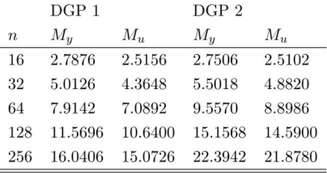
for both yt and ut: My and Mu.10 In Table 1 we report the average optimal blocklengths
for the two DGPs.
DGP 1 DGP 2 n My Mu My Mu 16 2.7876 2.5156 2.7506 2.5102 32 5.0126 4.3648 5.5018 4.8820 64 7.9142 7.0892 9.5570 8.8986 128 11.5696 10.6400 15.1568 14.5900 256 16.0406 15.0726 22.3942 21.8780
Table 1: Optimal blocklengths
9Notice that the case n = M = 16 is not taken into consideration as it equivalent to M = 1.
10The blocklength and the number of resulting blocks could be di¤erent for the two series. In order to overcome this issue, the data are wrapped around a circle and extra observations are used from the beginning of the series in order to have the same number of blocks (similar procedures are suggested in Davison and Hinkley, 1997, pp. 396-397).
We compute an estimate for 0 in …ve di¤erent ways. The …rst is a simple sample mean ^ = y = 1 n n X t=1 yt:
The second is an e¢ cient two step GMM estimator with two moment conditions
^ = arg min ^g ( )0 ^ 1
^ g ( )
where ^g ( ) = 1nPnt=1 yt ; ut 0
. The matrix of weights ^ is a Newey-West matrix evaluated at a certain consistent estimator of , . The remaining three estimators are weighted averages based on GEL estimators, i.e. the EL, the ET and the EU estimator,
^ =
b
X
i=1
^BGELi zi
where zi =PMj=1y(i 1)L+j. Given the auxiliary information wi =PMj=1u(i 1)L+j, the three
BGEL estimators for the probabilities are de…ned as
^ELi = 1 b 1 + ^ELwi ^ETi = exp ^ETwi Pb j=1exp ^ ET wj ^EUi = 1 b 1 ^EU(w i w) where w = 1b Pbi=1wi. ^ EL
and ^ET are computed numerically, while it is available a close form solution for ^EU. Each weighted estimator is computed for di¤erent values of M , where M goes from 2 to 16 and for an optimal M . The calculations are carried out in R and are based on 5000 Monte Carlo repetitions.
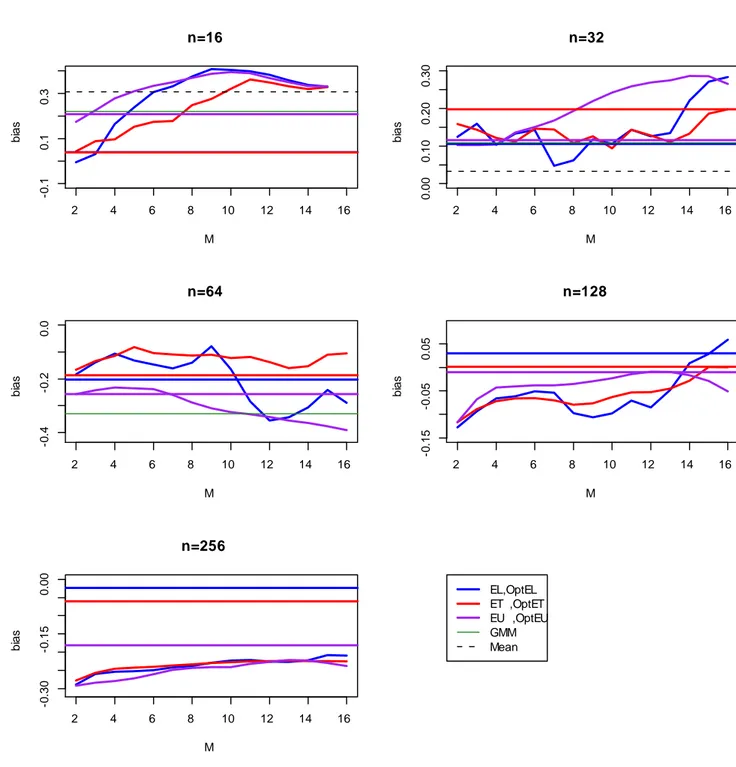
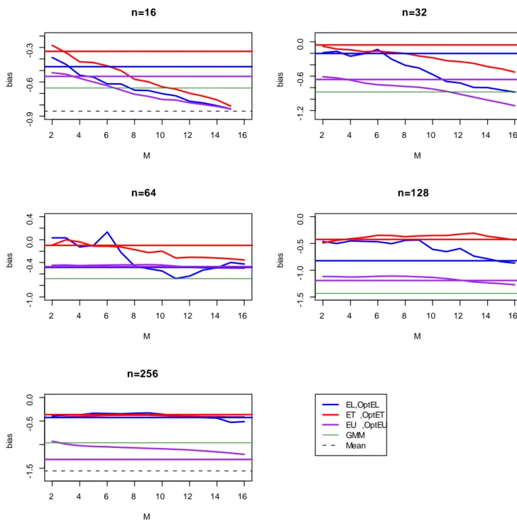
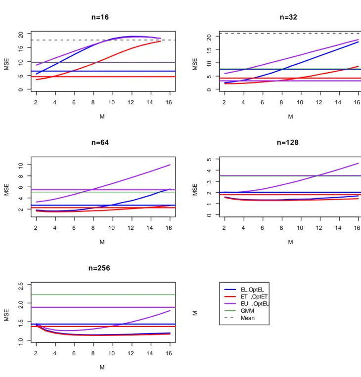
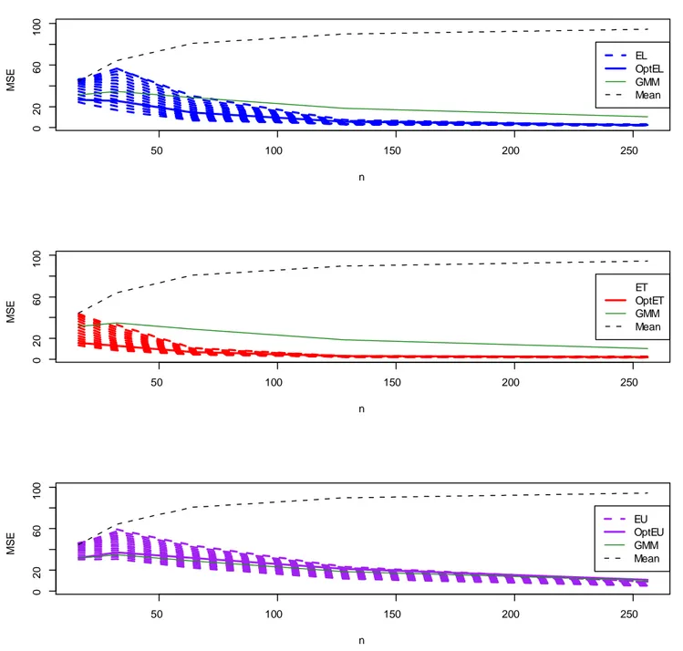
The results of the simulations are summarized in the appendix. Figures 1 to 4 describe the behaviour of the weighted estimators as the blocklength changes compared to those estimators that are independent of M , represented by the horizontal lines. In particular, the thick horizontal lines denote the weighted estimators based on My and Mu and, therefore,
denoted as OptEL, OptET , and OptEU . In several cases the sample mean is too far apart from the other estimators and it is not included in the graphs. Figures 5 to 8 describe the behaviour of all estimators as the sample size increases. Particularly when the sample size is small, the choice of M has a considerable impact on bias and MSE. For the latter (Figures 3 and 4), we see that the MSE tends to grow with M , while as n increases the slope of the curves corresponding to the EL and ET estimators becomes smaller and collapses to OptEL and OptET . On the other hand, the EU-based estimator is upward-sloping also for n = 256. In Figure 5 we see that the bias does not change much for the weighted estimators and for the GMM estimator. For DGP 2 the bias varies substantially for the EL-based estimator. The bias of the ET-based estimator, however, is less sensitive to the choice of M , while the EU-based estimator has a quite persistent negative bias and tends to behave as the GMM estimator. Given the appropriate di¤erence in scale, Figures 7 and 8 describe the same picture: the e¤ect of an arbitrary choice of M could have a large impact on the MSE in small samples. Such an e¤ect is more prominent for the EL case and the EU case. For the latter it persists also for larger values of n. Overall the EL estimator and the ET estimator that use an optimal blocklength have smaller MSE than GMM. Apart from small values of n, the EU estimator that uses an optimal blocklength is very similar to the GMM estimator. The MSE for the sample mean is the largest in the panel and tends to grow with the sample size.
5
Conclusion
In this paper we propose a two step procedure for Z-estimators in the presence of weakly dependent data and auxiliary information based on the estimation of BGEL probabilities. This procedure is attractive from di¤erent points of view. First of all, the computation of the BGEL probabilities is very simple, as it contemplates only the convex part of the BGEL problem (this is, the estimation of the Lagrange multiplier ). Moreover, whenever the Z-estimator is asymptotically equivalent to a GMM estimator (QS), it does not entail the well-known small sample e¤ects that a¤ect GMM estimators (see for example Altonji and Segal, 1996). Our asymptotic results state that the resulting Z-estimator is consistent and Normally distributed. The resulting variance depends on the relevance of the auxiliary information. In addition, we demonstrate that the estimator of a distribution based on the BGEL weights enjoys the same favourable features of the abovementioned Z-estimator. Furthermore, by means of Monte Carlo experiments, we describe how to apply our ap-proach to a standard time series problem. The laboratory we set is a location parameter estimation problem, similar to what is described in QS (see also Zhang, 1995). We compare three BGEL weighted estimators against a simple sample mean and an augmented GMM estimator, and we analyze their behaviour for di¤erent values of M and n. We argue that an appropriate choice of M is crucial in particular when the sample is small; because of that we advocate the use of data driven procedures for the selection of the blocklength (see Politis and White, 2004). The simulation results suggest that, in general, weighted esti-mators (in particular those based on ET) combined with an optimal blocklength improve over the competing estimators.
References
[1] Altonji, J. G., L. M. Segal (1996): Small-sample bias in GMM estimation of covariance structures, Journal of Business and Economic Statistics, 14, 353-366.
[2] Bravo, F. (2008): E¢ cient M-estimators with auxiliary information, University of York Working Paper.
[3] Bravo, F. (2009): Blockwise generalized empirical likelihood inference for non-linear dynamic moment conditions models, The Econometrics Journal, 12, 208-231.
[4] Chamberlain, G. (1987): Asymptotic e¢ ciency in estimation with conditional moment restrictions, Journal of Econometrics, 34, 305-334.
[5] Chen, J. J. Qin (1993): Empirical likelihood estimation for …nite populations and the e¤ective usage of auxiliary information, Biometrika, 80, 107-116.
[6] Crudu, F. (2009): GMM, Generalized Empirical Likelihood, and Time Series, Working Paper CRENoS.
[7] Davison, A. C., D. V. Hinkley (1997): Bootstrap Methods and their Applications, CUP. [8] Fitzenberger, B. (1997), The moving blocks bootstrap and robust inference for linear
least squares and quantile regression, Journal of Econometrics, 82, 235-287.
[9] Hansen, L. P. (1982): Large sample properties of generalized method of moments estimator, Econometrica, 50, 1029-1054.
[10] Hay…eld, T., J. S. Racine (2008): Nonparametric Econometrics: The np Package, Journal of Statistical Software 27, URL http://www.jstatsoft.org/v27/i05/.
[11] Hellerstein, J. G. W. Imbens (1999): Imposing moment restrictions from auxiliary data by weighting, Review of Economics and Statistics, 81, 1-14.
[12] Ibragimov, I. A., Y. V. Linnik (1971): Independent and Stationary Sequences of Ran-dom Variables. Wolters-Noordho¤, Groningen.
[13] Imbens, G. W. (1992): An e¢ cient method of moments estimator for discrete choice models with choice-based sampling, Econometrica, 60, 1187-1214.
[14] Imbens, G. W., T. Lancaster (1994): Combining micro and macro data in microecono-metric models, Review of Economic Studies, 61, 655-680.
[15] Kitamura, Y. (1997): Empirical likelihood methods with weakly dependent processes, The Annals of Statistics, 25, 2084-2102.
[16] Kuk, A. Y. C., T. K. Mak (1989): Median estimation in the presence of auxiliary information, Journal of the Royal Statistical Society B, 51, 261-269.
[17] Newey, W. K., D. McFadden (1994): Large sample estimation and hypothesis testing, in Handbook of Econometrics vol. IV, ed. R. Engle and D. McFadden. North Holland. [18] Newey, W. K., R. J. Smith (2004): Higher order properties of GMM and generalized
empirical likelihood estimators, Econometrica, 72, 219-255.
[19] Newey, W. K., K. West (1987): A simple positive semide…nite heteroskedasticity and autocorrelation consistent covariance matrix, Econometrica, 55, 703-708.
[20] Owen, A. B. (2001): Empirical Likelihood, Chapman-Hall.
[21] Pakes, A., O. Linton (2001): Nonlinear Methods for Econometrics, LSE lecture notes, URL http://econ.lse.ac.uk/sta¤/olinton/ec481/aet.pdf.
[22] Pakes, A., D. Pollard (1989): Simulation and the asymptotics of optimization estima-tors, Econometrica, 57, 1027-1057.
[23] Patton, A., D. N. Politis, H. White (2009): CORRECTION TO “Automatic Block-Length Selection for the Dependent Bootstrap” by D. Politis and H. White, Econo-metric Reviews, 28, 372-375.
[24] Politis, D. N., J. P. Romano, On the Sample Variance of Linear Statistics Derived from Mixing Sequences, Stochastic Processes and Their Applications, 45, 155-167. [25] Politis, D. N., H. White (2004): Automatic block-length selection for the dependent
bootstrap, Econometric Reviews, 23, 53-70.
[26] Qian, H., P. Schmidt (1999): Improved instrumental variables and generalized method of moments estimators, Journal of Econometrics, 91, 145-169.
[27] Smith, R. J. (2004): GEL criteria for moment condition models, cemmap Working Paper.
[28] Van der Vaart, A. (2007): Asymptotic Statistics, CUP.
[29] Zhang, B. (1995): M-estimation and quantile estimation in the presence of auxiliary information, Journal of Statistical Planning and Inference, 44, 77-94.
6
Appendix: Proofs and Figures
In what follows we present the proofs of the theorems presented in Section 3 and some auxiliary results. In addition, we use the following notation: !p and !d denote
con-vergence in probability and concon-vergence in distribution; C is a generic positive constant; CS and T denote Cauchy-Schwarz inequality and triangular inequality respectively; k k is the Euclidean norm of . The sums Pi and Pj substitute Pbi=1 and Pbj=1, while Pt substitutes Pnt=1. The CLT is meant to be a CLT for strong mixing sequences (see e.g. Ibragimov and Linnik, 1971) and CMT is the continuous mapping theorem.
Proof of Lemma 1. Consider again ^ R ( ) = 1 b X i ( 0gi) :
Notice that ^R ( )is concave through ( ). Moreover, assumptions 2 to 4 match assumptions (i)-(iii) from Theorem 2.7 of Newey and McFadden (1994). Then, consistency of ^ follows. Consider now a mean value expansion of the …rst order conditions of the BGEL criterion function, 0 = @ ^R ^ @ = 1 b X i 1 _ 0 gi gi = g + M b X i 1 _ 0 gi gigi0 ! ^ M
where g = Pigi=b. Since ^ is consistent and _ ^ , we have that 1 _ 0 gi = 1 + op(1). Thus, multiplying by pn 0 = png ^ pn ^ M op(1) ^ p n ^ M
where ^ = MPigig0i=b. Notice that ^
p nM^ = Op(1); therefore, by rearranging p n ^ M = ^ 1png + o p(1) : (6)
Finally, by applying CLT topng and Slutsky theorem, the result follows.
Proof of Theorem 1 (Consistency of ^ ). Let us compute a mean value expansion of ^i = 1 ^ 0 gi P j 1 ^ 0 gj
about = 0, where ^ is a consistent estimator for : ^i = 1 b + 1 b 0 B @ 2 _0g i g0i 1 b P j 1 _ 0 gj 1 ^ 0 gi 1b P j 2 _ 0 gj g0j 1 b P j 1 _ 0 gj 2 1 C A ^ 0 = 1 b + 1 b 0 B @ 2 _0g i ^ 0 gi 1 b P j 1 _ 0 gj 1 ^ 0 gi 1b Pj 2 _ 0 gj ^ 0 gj 1 b P j 1 _ 0 gj 2 1 C A :
From results of Lemma 1 we obtain
^i = 1 b + 1 b ^0g i+ op(1) (7) and ^i = 1 b (1 + op(1)) : (8)
From Lemma 1 in Crudu (2009) we have ^h ( ) = ^m ( ) + Op(M=n). Then, by adding
and subtracting ^h ^ and T
m ^ m ^ ^h ^ + ^h ^
Moreover, by optimality of ^ and since m ( 0) = 0, and by repeated application of Lemma 1 in Crudu (2009) and T m ^ m ^ m ^^ + (1 + op(1))k ^m ( 0) m ( 0)k + Op M n sup 2Bkm ( ) ^ m ( )k + (1 + op(1)) sup 2Bk ^ m ( ) m ( )k + Op M n :
By Assumption 3 sup 2Bkm ( ) m ( )^ k = op(1); hence
Since m ( ) is bounded away from zero for k 0k > (assumption 2), it follows that
^ 2 k 0k < . As is arbitrary, ^ !p 0:
Proof of Theorem 2 (Asymptotic Normality of ^ ). Let us considerPi^ihi ^ =
0; by replacing the probabilities with the expression in 7
0 = 1 b
X
i
1 + ^0gi+ op(1) hi ^
and mean value expand hi ^ about 0, for ^ being consistent
0 = X i 1 + ^0gi+ op(1) hi ^ = X i 1 + ^0gi 0 @hi( 0) + @hi _ @ ^ 0 1 A + op(1) ^h ^
where _ 0 ^ 0 . Let us de…ne ^B ( ) = M
P
ihi( ) gi0=b. Then, by
appropri-ate rescaling and (6)
0 = pn^h ( 0) + ^B ( 0) ^ 1png + 0 @1 b X i @hi _ @ + ^ 0X i gi @hi( 0) @ =b 1 A pn ^ 0 +op(1)pn^h ^ = A1+ A2+ A3 where A1 = p n^h ( 0) + ^B ( 0) ^ 1png; A2 = X i @hi _ =@ + ^ 0X i gi@hi( 0) =@ =b ! p n ^ 0 ;
A3 = op(1)
p
n^h ^ :
From assumption 3 and Lemma 1 in Crudu (2009)pn^h ( 0)!dN (0; S ( 0))and
p ng!d
N (0; ). Then, after simple calculations, we get A1 !d N (0; W ), where
W = I; B ( 0) 1 0 B @ S ( 0) B ( 0) B ( 0)0 1 C A 0 B @ I 1B ( 0)0 1 C A = S ( 0) B ( 0) 1B ( 0)0
Let us now focus attention on A2. By Lemma 1 in Crudu (2009) and T
^01 b X i gi @hi _ @ 0 ^ 1 n X t ft @mt _ @ 0 + Op M n ^ 1 n X t sup 2B ft @mt( ) @ 0 + op(1) : Thus, ^01 b X i gi @hi _ @ op(1) :
By CMT and assumption 3 pn^h ^ is Normally distributed. Thus, its order of magni-tude is Op(1) and A3 = op(1). Finally,
M ( 0)0pn ^ 0 = I; B (^ 0) 1 0 B @ p n^h ( 0) p ng 1 C A + op(1) and p n ^ 0 = M ( 0)0 1 I; B (^ 0) 1 0 B @ p n^h ( 0) p ng 1 C A + op(1)
which implies, by CLT applied to png, assumption 3 and CMT, p
n ^ 0 !d N 0; M ( 0)0 1
S ( 0) B ( 0) 1B ( 0)0 (M ( 0)) 1 :
Proof of Corollary 1. From results in Lemma 1 and Theorem 1 we have
^ (z) = 1 b X i 1M (zi z) 1 + ^ 0 gi+ op(1) = ^b(z) png0^ 1pM nb X i gi1M(zi z) + op 1 p n
Then, by adding and subtracting (x) and multiplying both sides bypn, we get p n (^ (z) (x)) = pn (^b(z) (x)) png0^ 11 b X i gi1M(zi z) + op(1) = 1; ^a0^ 1 0 B @ p n (^b(z) (x)) png 1 C A + op(1) ! dN 0; 2 a0 1a :
2 4 6 8 10 12 14 16 -0 .1 0 .1 0 .3 M bi as n=16 2 4 6 8 10 12 14 16 0. 00 0. 10 0. 20 0. 30 M bi as n=32 2 4 6 8 10 12 14 16 -0 .4 -0 .2 0 .0 M bi as n=64 2 4 6 8 10 12 14 16 -0 .15 -0 .05 0. 05 M bi as n=128 2 4 6 8 10 12 14 16 -0 .30 -0 .15 0. 00 M bi as n=256 EL,OptEL ET ,OptET EU ,OptEU GMM Mean
2 4 6 8 10 12 14 16 -0 .9 -0 .6 -0 .3 n=16 M bi as 2 4 6 8 10 12 14 16 -1 .2 -0 .6 0 .0 n=32 M bi as 2 4 6 8 10 12 14 16 -1 .0 -0 .4 0 .0 0 .4 n=64 M bi as 2 4 6 8 10 12 14 16 -1 .5 -1 .0 -0 .5 0 .0 n=128 M bi as 2 4 6 8 10 12 14 16 -1 .5 -0 .5 0 .0 n=256 M bi as EL,OptEL ET ,OptET EU ,OptEU GMM Mean
2 4 6 8 10 12 14 16 0 5 10 15 20 n=16 M MSE 2 4 6 8 10 12 14 16 0 5 10 15 20 n=32 M MSE 2 4 6 8 10 12 14 16 2 4 6 8 10 n=64 M MSE 2 4 6 8 10 12 14 16 0 1 2 3 4 5 n=128 M MSE 2 4 6 8 10 12 14 16 1 .0 1 .5 2 .0 2 .5 n=256 M MSE M EL,OptEL ET ,OptET EU ,OptEU GMM Mean
2 4 6 8 10 12 14 16 10 30 50 n=16 M MSE 2 4 6 8 10 12 14 16 0 20 40 60 n=32 M MSE 2 4 6 8 10 12 14 16 0 10 20 30 40 n=64 M MSE 2 4 6 8 10 12 14 16 5 10 20 n=128 M MSE 2 4 6 8 10 12 14 16 2 4 6 8 10 n=256 M MSE EL,OptEL ET ,OptET EU ,OptEU GMM Mean
50 100 150 200 250 -1 .5 -0 .5 0 .5 n bi as EL OptEL GMM Mean 50 100 150 200 250 -1 .5 -0 .5 0 .5 n bi as ET OptET GMM Mean 50 100 150 200 250 -1 .5 -0 .5 0 .5 n bi as EU OptEU GMM Mean
50 100 150 200 250 -3 .0 -2 .0 -1 .0 0 .0 n bi as EL OptEL GMM Mean 50 100 150 200 250 -3 .0 -2 .0 -1 .0 0 .0 n bi as ET OptET GMM Mean 50 100 150 200 250 -3 .0 -2 .0 -1 .0 0 .0 n bi as EU OptEU GMM Mean
50 100 150 200 250 5 10 20 n MSE EL OptEL GMM Mean 50 100 150 200 250 5 10 20 n MSE ET OptET GMM Mean 50 100 150 200 250 5 10 20 n MSE EU OptEU GMM Mean
50 100 150 200 250 0 20 60 1 00 n MSE EL OptEL GMM Mean 50 100 150 200 250 0 20 60 1 00 n MSE ET OptET GMM Mean 50 100 150 200 250 0 20 60 1 00 n MSE EU OptEU GMM Mean
Ultimi Contributi di Ricerca CRENoS
I Paper sono disponibili in:Uhttp://www.crenos.itU
10/21 Francesco Lippi, Fabiano Schivardi, “Corporate Control and Executive Selection”
10/20 Claudio Detotto, Valerio Sterzi, “The role of family in suicide rate in Italy”
10/19 Andrea Pinna, “Risk-Taking and Asset-Side Contagion in an Originate-to-Distribute Banking Model”
10/18 Andrea Pinna, “Optimal Leniency Programs in Antitrust”
10/17 Juan Gabriel Brida, Manuela Pulina, “Optimal Leniency Programs in Antitrust”
10/16 Juan Gabriel Brida, Manuela Pulina, Eugenia Riaño, Sandra Zapata Aguirre “Cruise visitors’ intention to return as land tourists and recommend a visited destination. A structural equation model”
10/15 Bianca Biagi, Claudio Detotto, “Crime as tourism externality”
10/14 Axel Gautier, Dimitri Paolini, “Universal service financing in competitive postal markets: one size does not fit all”
10/13 Claudio Detotto, Marco Vannini, “Counting the cost of crime in Italy”
10/12 Fabrizio Adriani, Luca G. Deidda, “Competition and the signaling role of prices”
10/11 Adriana Di Liberto “High skills, high growth: is tourism an exception?”
10/10 Vittorio Pelligra, Andrea Isoni, Roberta Fadda, Iosetto Doneddu, “Social Preferences and Perceived Intentions. An experiment with Normally Developing and
Autistic Spectrum Disorders Subjects”
10/09 Luigi Guiso, Luigi Pistaferri, Fabiano Schivardi, “Credit within the firm”
10/08 Luca Deidda, Bassam Fattouh, “Relationship Finance, Market Finance and Endogenous Business Cycles” 10/07 Alba Campus, Mariano Porcu, “Reconsidering the
well-being: the Happy Planet Index and the issue of missing data”
10/06 Valentina Carta, Mariano Porcu, “Measures of wealth and well-being. A comparison between GDP and ISEW” 10/05 David Forrest, Miguel Jara, Dimitri Paolini, Juan de Dios
Tena, “Institutional Complexity and Managerial Efficiency: A Theoretical Model and an Empirical Application”
10/04 Manuela Deidda, “Financial Development and Selection into Entrepreneurship: Evidence from Italy and US” 10/03 Giorgia Casalone, Daniela Sonedda, “Evaluating the
Distributional Effects of the Italian Fiscal Policies using Quantile Regressions”
10/02 Claudio Detotto, Edoardo Otranto, “A Time Varying Parameter Approach to Analyze the Macroeconomic Consequences of Crime”
10/01 Manuela Deidda, “Precautionary saving, financial risk and portfolio choice”
09/18 Manuela Deidda, “Precautionary savings under liquidity constraints: evidence from Italy”
Finito di stampare nel mese di Novembre 2010 Presso studiografico&stampadigitale Copy Right Via Torre Tonda 8 – Tel. 079.200395 – Fax 079.4360444