Experimental Investigation on Fluid Mechanics
of Different Micro Heat Transfer Devices
Year 2019/2020
XXXII PhD Course of
Theoretical and Applied Mechanics
Supervisor: Prof. Giovanni Paolo Romano
PhD student: Michela Spizzichino
2 Summary Summary ... 2 Index of Figures ... 3 Index of Tables ... 7 Abstract ... 8
Chapter 1 - Introduction and Problem Statement ... 9
Chapter 2 - Background and definitions ... 16
2.1 Friction factor and micro-cell efficiency ... 24
2.2 Entropy analysis ... 26
Chapter 3 - Materials and experimental methods ... 28
3.1 Micro Devices ... 29
3.1.1 Straight channel micro-cell ... 33
3.1.2 Straight parallel channels micro-cell type-I ... 34
3.1.3 Straight parallel channels micro-cell type-II ... 37
3.1.4 Standard serpentine micro-cell ... 39
3.1.5 Wavy-sinusoidal serpentine micro-cell ... 42
3.2 Syringe Pump ... 44
3.2.1 Flow rate studied ... 45
3.3 Hot Plate ... 47 3.4 Infrared Thermometer ... 49 3.5 Thermocouples Reader ... 50 3.6 Tracer ... 51 3.7 Fast-Cam ... 52 3.8 Pressure Sensor ... 55
3.9 Determination of Reynolds number ... 55
3.10 Determination of Nusselt number ... 59
Chapter 4 - Results: Thermal Measurements ... 64
4.1 Temperature experimental data ... 65
4.2 Temperature extrapolated data ... 71
4.3 Thermal measurements results ... 75
4.4 Error analysis results ... 81
Chapter 5 – Fanning Friction Factors and Efficiencies ... 85
5.1 Efficiency parameter ... 91
Chapter 6 - µPIV Results ... 94
6.1 Configurations selection for analysis ... 95
3
6.3 Mean Standard deviation and vorticity fields ... 102
6.4 Mean velocity vectors, magnitude and vorticity fields at 90 ml/min ... 108
6.5 Vertical Profiles of standard serpentine cells ... 111
6.6 Mean Entropy fields ... 114
Chapter 7 – Conclusions ... 118
Appendix ... 121
A.1 Interpolation and extrapolation method ... 121
A.2 Error analysis: Reynolds and Nusselt numbers ... 124
A.3 Particle Image Velocimetry analysis and post-processing ... 127
A.4 Measured temperatures of outlet fluid and wall ... 131
A.5 Extrapolated temperatures of outlet fluid and wall ... 134
A.6 Prandtl Number ... 137
A.7 Efficiency parameters ... 140
Acknowledgements ... 144
References ... 145
Index of Figures Figure 1: Interferograms of square ducts with radii at the corners, Compact Heat Exchangers, F.Mayinger, J. Klas (1993) [7]... 10
Figure 2: Example of corrugated walls (a), cylindrical ribs (b) and channel side grooving (c); [8], [9], [10]. 10 Figure 3: Development of a micro-heat exchanger with stacked plates using LTCC technology, E. Vásquez-Alvarez, F. T. Degasperi, L. G. Morita, M. R. Gongora-Rubio, R. Giudici (2010) [11]. ... 11
Figure 4: Micro-PIV visualization and numerical simulation of flow and heat transfer in three micro pin-fin heat sinks, G. Xia, Z. Chen, L. Cheng, D. Ma, Y. Zhai, Y. Yang (2017) [16]. ... 13
Figure 5: Hydrodynamic and thermal boundary layers for flow over a heated flat plate - Engineering Thermofluids - M. Massoud [2]. ... 19
Figure 6: Example of comparison of the Average Nusselt numbers as a function of the Reynolds number obtained for three tested micro-cells at 50 °C. ... 23
Figure 7: Sketch of the experimental setup. ... 28
Figure 8: Geometrical configurations studied. ... 30
Figure 9: Example of a sealing frame manufactured on the straight parallel channels cell type-I. ... 31
Figure 10: Straight channel cell with aluminum gap-pad. ... 31
Figure 11: Inlet and exit tubes. ... 32
Figure 12: Top view and CAD drawing of the straight channel micro-cell. ... 33
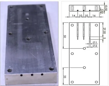
Figure 13: View of the aluminum bottom side and CAD drawing of the thermocouples venues. ... 34
Figure 14: Top view and CAD drawing of the straight parallel channels micro-cell type-I. ... 36
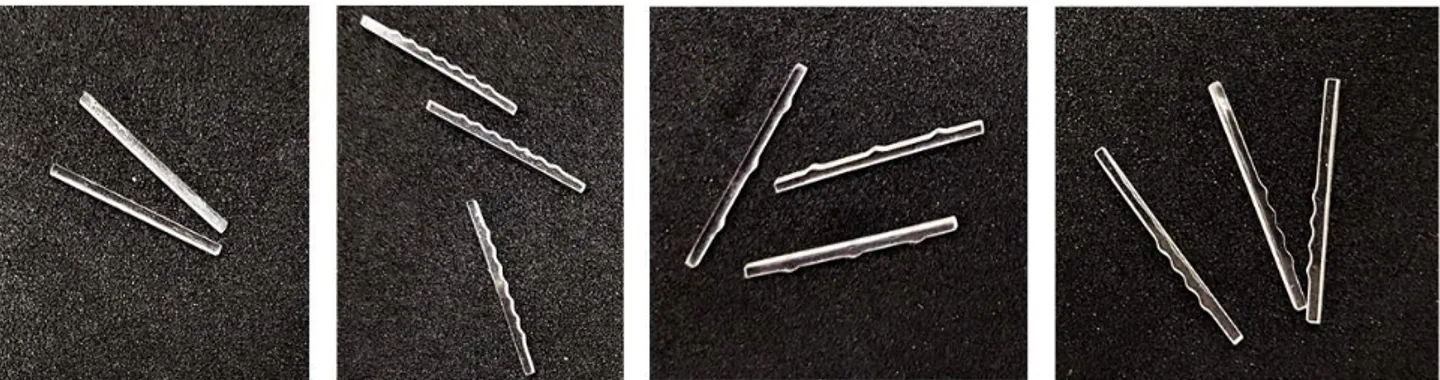
Figure 15: Fluid guide profiles and the placement scheme with flow rate percentages. ... 36
Figure 16: Top view of the aluminum straight parallel channels micro-cell type-I. ... 37
Figure 17: Top view and CAD drawing of the straight parallel channels micro-cell type-II. ... 38
4
Figure 19: Top view and CAD drawing of the standard serpentine cell. ... 40
Figure 20: View of the aluminum bottom side and CAD drawing of the thermocouples venues. ... 41
Figure 21: Standard serpentine micro-cell with ribs. (a) Top view of the test section; (b) View in the cross-section with rib. ... 42
Figure 22: Top view and CAD drawing of the wavy-sinusoidal serpentine. ... 43
Figure 23: Hll Landgraf LA-800 Syring Pump. ... 44
Figure 24: Modified 140 ml aluminum syringe. Lateral view (left image) and front view (right image). ... 45
Figure 25: Hot plate Stuart US-150. ... 48
Figure 26: Infrared thermometer PCE 779N. ... 49
Figure 27: K, J, E, T, N and R-type thermocouple reader SE521. ... 50
Figure 28: Sample of hollow glass spherical particles. ... 52
Figure 29: Fast-cam Mini AX100 and Nikon objectives. ... 53
Figure 30: Flowplus16-ViscoTec pressure sensor, on the left. Elveflow OB1-MK3, on the right. ... 55
Figure 31: Water temperatures as a function of time [s] and flow rate [ml/min] for the standard serpentine cell at 50 °C. ... 66
Figure 32: Wall temperatures as a function of time [s] and flow rate [ml/min] for the standard serpentine cell at 50 °C. ... 66
Figure 33: Water temperatures as a function of time [s] and flow rate [ml/min] for the standard serpentine cell at 70 °C. ... 67
Figure 34: Wall temperatures as a function of time [s] and flow rate [ml/min] for the standard serpentine cell at 70 °C. ... 67
Figure 35: Water temperatures as a function of time [s] and flow rate [ml/min] for the straight channel cell at 50 °C. ... 69
Figure 36: Outlet water temperatures as a function of flow rate [ml/min] for the parallel channels cell realized in plexiglass and aluminum at 50 °C... 70
Figure 37: Extrapolated water temperatures as a function of time [s] and flow rate [ml/min] for the standard serpentine cell at 50 °C. ... 71
Figure 38: Extrapolated wall temperatures as a function of time [s] and flow rate [ml/min] for the standard serpentine cell at 50 °C. ... 72
Figure 39: Extrapolated water temperatures as a function of time [s] and flow rate [ml/min] for the standard serpentine cell at 70 °C. ... 72
Figure 40: Extrapolated wall temperatures as a function of time [s] and flow rate [ml/min] for the standard serpentine cell at 70 °C. ... 73
Figure 41: New extrapolation of wall temperatures as a function of time [s] and flow rate [ml/min] for the standard serpentine cell at 50 °C. ... 75
Figure 42: Comparison of the Average Nusselt numbers as a function of the Reynolds number obtained for straight channel cell at 50 °C with the results proposed by Lee and Garimella [41], [42]. ... 76
Figure 43: Comparison of the Average Nusselt numbers as a function of the Reynolds number obtained for the three tested micro-cells at 50 °C with the classical correlation proposed by Sieder & Tate [39]. ... 77
Figure 44: Comparison of the Average Nusselt numbers as a function of the Reynolds number obtained for the three tested micro-cells at 70 °C with the classical correlation proposed by Sieder & Tate [39]. ... 77
Figure 45: Comparison of the Average Nusselt numbers as a function of the Reynolds number obtained for the four tested micro-cells at 50 °C with the classical correlation proposed by Sieder & Tate [39]. ... 79
Figure 46: Comparison of the Average Nusselt numbers as a function of the Reynolds number obtained for the four tested micro-cells at 70 °C with the classical correlation proposed by Sieder & Tate [39]. ... 80
Figure 47: Error on Nusselt number (ΔNu) as a function of Reynolds number for all micro-cells at 50 °C. .... 82
Figure 48: Error on Nusselt number (ΔNu) as a function of Reynolds number for all micro-cells at 70 °C. .... 83
5
Figure 50: Fanning friction factor as a function of Reynolds number for the tested micro-channels at 70 °C: parallel channels, standard serpentine with and without ribs, wavy-sinusoidal serpentine, with the classical correlation proposed by J.T. Fanning [46]. ... 87 Figure 51: Fanning friction factor as a function of Reynolds number for the tested micro-channels at 70 °C: standard serpentine tested with water and water-glycerin solutions, with the classical correlation proposed by J.T. Fanning [46]. ... 88 Figure 52: Comparison of the efficiency parameters as a function of Reynolds number for the three tested micro-cells at 50 °C. ... 91 Figure 53: Comparison of the efficiency parameters as a function of Reynolds number for the three tested micro-cells at 70 °C. ... 91 Figure 54: Flow distribution in the parallel channels cell type-I vs parallel channels cell type-II (inner and outer sections of the six first channels, figure 55). ... 96 Figure 55: Flow rate of 30 ml/min. Acquisition areas delimited in blue with main technical features (left column) and picture (right column) of the top view of the micro-cells. A) straight parallel channels type-II, B) standard serpentine, C) wavy-synusoidal serpentine. In red the area whose technical details are shown in the lower left panel. ... 97 Figure 56: Flow rate of 90 ml/min. Acquisition areas delimited in blue with main technical features (left column) and picture (right column) of the top view of the micro-cells. A) straight parallel channels type-II, B) standard serpentine, C) wavy-synusoidal serpentine. In red the area whose technical details are shown in the lower left panel. ... 98 Figure 57: Mean velocity vectors fields at 30 ml/min. (a) straight parallel channels, (b) standard serpentine, (c) wavy serpentine, d) std. serpentine with 70 % water & 30 % glycerin, e) std. serpentine with 30 % water & 70 % glycerin. ... 100 Figure 58: Mean velocity magnitude color maps at 30 ml/min. (a) straight parallel channels, (b) standard serpentine, (c) wavy serpentine, d) std. serpentine with 70 % water & 30 % glycerin, e) std. serpentine with 30 % water & 70 % glycerin. ... 101 Figure 59: Standard Deviation of u component at 30 ml/min. a) straight parallel channels type-II, b) standard serpentine, c) wavy-synusoidal serpentine, d) std. serpentine with 70 % water & 30 % glycerin, e) std. serpentine with 30 % water & 70 % glycerin . ... 103 Figure 60: Standard Deviation of v component at 30 ml/min. a) straight parallel channels type-II, b) standard serpentine, c) wavy-synusoidal serpentine, d) std. serpentine with 70 % water & 30 % glycerin, e) std. serpentine with 30 % water & 70 % glycerin. ... 104 Figure 61: Standard Deviation of u component at 90 ml/min. a) straight parallel channels type-II, b) standard serpentine, c) wavy-synusoidal serpentine, d) std. serpentine with 70 % water & 30 % glycerin, e) std. serpentine with 30 % water & 70 % glycerin. ... 105 Figure 62: Standard Deviation of v component at 90 ml/min. a) straight parallel channels type-II, b) standard serpentine, c) wavy-synusoidal serpentine, d) std. serpentine with 70 % water & 30 % glycerin, e) std. serpentine with 30 % water & 70 % glycerin. ... 106 Figure 63: Mean vorticity color maps at 30 ml/min. (a) straight parallel channels, (b) standard serpentine, (c) wavy serpentine, d) std. serpentine with 70 % water & 30 % glycerin, e) std. serpentine with 30 % water & 70 % glycerin. ... 107 Figure 64: Mean velocity vectors fields at 90 ml/min. (a) straight parallel channels, (b) standard serpentine, (c) wavy serpentine, d) std. serpentine with 70 % water & 30 % glycerin, e) std. serpentine with 30 % water & 70 % glycerin. ... 109 Figure 65: Mean velocity magnitude color maps at 90 ml/min. (a) straight parallel channels, (b) standard serpentine, (c) wavy serpentine, d) std. serpentine with 70 % water & 30 % glycerin, e) std. serpentine with 30 % water & 70 % glycerin. ... 110
6
Figure 66: Mean vorticity color maps at 90 ml/min. (a) straight parallel channels, (b) standard serpentine, (c) wavy serpentine, d) std. serpentine with 70 % water & 30 % glycerin, e) std. serpentine with 30 % water & 70 % glycerin. ... 111 Figure 67: Standard serpentine geometry. Sections for the analysis of vertical profiles. ... 112 Figure 68: Comparison of vertical profiles extracted at position 1. Std. serpentine tested with water (red curve), std. serpentine tested with 70 % water and 30 % glycerin (blue curve) and std. serpentine tested with 30 % water and 70 % glycerin. ... 112 Figure 69: Comparison of vertical profiles extracted at position 2. Std. serpentine tested with water (red curve), std. serpentine tested with 70 % water and 30 % glycerin (blue curve) and std. serpentine tested with 30 % water and 70 % glycerin. ... 113 Figure 70: Comparison of vertical profiles extracted at position 3. Std. serpentine tested with water (red curve), std. serpentine tested with 70 % water and 30 % glycerin (blue curve) and std. serpentine tested with 30 % water and 70 % glycerin. ... 113 Figure 71: Mean entropy fields at 30 ml/min. (a) straight parallel channels, (b) standard serpentine, (c) wavy serpentine, d) std. serpentine with 70 % water & 30 % glycerin, e) std. serpentine with 30 % water & 70 % glycerin. ... 115 Figure 72: Mean entropy fields at 90 ml/min. (a) straight parallel channels, (b) standard serpentine, (c) wavy serpentine, d) std. serpentine with 70 % water & 30 % glycerin, e) std. serpentine with 30 % water & 70 % glycerin. ... 116 Figure 73: Wavy-sinusoidal serpentine cell, before (left) and after (right) the minimum subtraction. ... 127 Figure 74: Wavy-sinusoidal serpentine cell raw image (top left), application of the exclusion mask (red area) with evidence of analysis windows (top right), instantaneous velocity vector fields (lower center). ... 128 Figure 75: Comparison of the average Nusselt numbers as a function of the Prandtl number obtained for the four micro-cells tested with water together with the reference law for a laminar flow over a flat isothermal plate [2]. Hot source temperature equal to 50 °C ... 1287 Figure 76: Comparison of the average Nusselt numbers as a function of the Prandtl number obtained for the two micro-cells tested with water/glycerin solutions together with the reference law for a laminar flow over a flat isothermal plate [2]. Hot source temperature equal to 50 °C. ... 1288 Figure 77: Comparison of the average Nusselt numbers as a function of the Prandtl number obtained for the four micro-cells tested with water together with the reference law for a laminar flow over a flat isothermal plate [2]. Hot source temperature equal to 70 °C ... 1288 Figure 78: Comparison of the average Nusselt numbers as a function of the Prandtl number obtained for the two micro-cells tested with water/glycerin solutions together with the reference law for a laminar flow over a flat isothermal plate [2]. Hot source temperature equal to 70 °C. ... 139 Figure 79: Comparison of the efficiency parameters ε'as a function of Reynolds number for the tested
cells at 50 °C.. ... 141 Figure 80: Comparison of the efficiency parameters ε''as a function of Reynolds number for the
tested cells at 50 °C.. ... 142 Figure 81: Comparison of the efficiency parameters ε'as a function of Reynolds number for the tested
cells at 70 °C.. ... 142 Figure 82: Comparison of the efficiency parameters ε''as a function of Reynolds number for the
7
Index of Tables
Table 1: 𝐷ℎ, L and 𝐷ℎ/ 𝐿 values for each micro-cell . ... 25
Table 2: Conversion factors from pixel to meter and from frame to second. ... 27
Table 3: Main features of the straight channel micro-cell. ... 33
Table 4: Main features of the straight parallel channels micro-cell type-I... 35
Table 5: Main features of the straight parallel channels micro-cell type-I... 38
Table 6: Main features of the standard serpentine cell. ... 40
Table 7: Main features of the wavy-sinusoidal serpentine cell. ... 43
Table 8: Listing of flow rates, Reynolds numbers and speed values analyzed for each micro-cell. ... 46
Table 9: Amount of values recorded as a function of flow rate starting by a fixed volume of 140 ml. ... 51
Table 10: Micro-cell type with indication of the correct dosage of tracer in grams. ... 52
Table 11: Summary of the set conditions. ... 54
Table 12: Reynolds number parameters. Cooling fluid: distilled water. ... 56
Table 13: Reynolds numbers and bulk velocity values. Cooling fluid: distilled water. ... 57
Table 14: Reynolds number parameters. Solution with 30 % glycerin & 70 % water. ... 58
Table 15: Reynolds number parameters. Solution with 70 % glycerin & 30 % water. ... 58
Table 16: Reynolds numbers and bulk velocity values obtained for the two tested solutions. ... 58
Table 17: Geometrical parameters of the tested micro-cells. ... 60
Table 18: Mass flow rate values corresponding to set flow rates for each working fluid. ... 61
Table 19: Glycerin and Ethylene glycol properties table. ... 63
Table 20: Geometrical parameters of the tested micro-cells. ... 88
Table 21: Bulk Velocities, Reynolds numbers and Fanning factors at 70 °C. ... 90
Table 22: Measurement time vs extrapolation time. ... 122
Table 23: PIVlab processing and vector validation times for different configurations. ... 129
Table 24: Final measured temperatures of outlet fluid for each flow rate [ml/min] and configuration at 50 °C. ... 131
Table 25: Final measured temperatures of wall for each flow rate [ml/min] and configuration at 50 °C. .. 132
Table 26: Final measured temperatures of outlet fluid for each flow rate [ml/min] and configuration at 70 °C. ... 132
Table 27: Final measured temperatures of wall for each flow rate [ml/min] and configuration at 70 °C. .. 133
Table 28: Final extrapolated temperatures of outlet fluid for each flow rate [ml/min] and configuration at 50 °C, with indication in red of anomalous values provided by analytical model. ... 134
Table 29: Final extrapolated temperatures of wall for each flow rate [ml/min] and configuration at 50 °C, with indication in red of anomalous values provided by analytical model. ... 135
Table 30: Final extrapolated temperatures of outlet fluid for each flow rate [ml/min] and configuration at 70 °C, with indication in red of anomalous values provided by analytical model. ... 135
Table 31: Final extrapolated temperatures of wall for each flow rate [ml/min] and configuration at 70 °C, with indication in red of anomalous values provided by analytical model. ... 136
8
Abstract
The future technological horizons for engineering applications (Automotive, Energy, Bio-engineering) will require the use of small size heat exchangers with high heat exchange efficiency. In the present work, the thermo-hydrodynamic behaviour of eight different micro-heat exchangers is investigated experimentally using thermal measurements and µPIV (micro Particle Image Velocimetry), in order to detail and improve the thermal performance of micro-devices. To test the heat transfer properties and the detailed fluid flow behaviour, this research was extended from typical range of Reynolds number in the laminar regime, from 50 to 1500, to the turbulent regime with Reynolds number up to 4000. Moreover, different cooling fluids are employed to analyse the heat transfer capability of micro-devices under different working conditions. Results are evaluated first in term of the Nusselt-Reynolds diagram and then through the efficiency of the cells performed by relating the average Nusselt number to the Fanning factor. On the base of the thermal analysis, the µPIV measurements were employed to detail the observed global heat exchange performances of each micro-cell configuration. In order to make a link with results highlighted by the thermal measurements the attention was focused on local fluid recirculation and acceleration as related to the specific geometry and to the different flow rates. The main result of this investigation is that the standard serpentine micro cell attains the highest efficiency regardless of flow regime, getting high Nusselt numbers combined with low pressure losses, as derived by the observation of quite high local velocities and few recirculation regions. In fact, PIV results highlighted that the main reason for the increasing Nusselt number is only dependent on local high intensity accelerations and not on recirculation regions, that appear to contribute only to pressure loss increments. Also in case of working fluids with high glycerin contents, e.g. 30 % water and 70 % glycerin, the results suggested high thermal exchange properties, mainly related to the glycerin physical properties and not only to local high intensity fluid accelerations.
9
Chapter 1 - Introduction and Problem Statement
The use of high efficiency heat exchangers is the basis of several technological developments required in different engineering applications, e.g. automotive, energy and bioengineering [1]. Since the heat transfer coefficient is inversely proportional to the characteristic dimension of the system, ℎ =𝑄̇𝐶𝑜𝑛𝑣
𝐴∙∆𝑇 [ W
m2∙K] [2], a valid solution to optimize the cooling process is to use a system of
multiple micro heat exchangers instead of a single macro counterpart. Until now, the main features usually investigated to enhance the heat transfer efficiency of micro-devices are related to the materials of the microchannel, the channel geometry, the cooling fluid and the flow regime ([3],[4]). To this aim, the heat transfer performances of a small-device are commonly assessed by the ratio between the heat transfer rate, usually expressed in terms of the average Nusselt number, based on the difference between inlet and outlet temperature of the working fluid, and the pressure losses induced by the geometry, which can be directly measured or analytically determined on the base of boundary conditions [5] (in section 2 exact definitions are given).
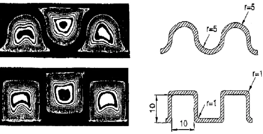
From the 90s up to today, several studies have been carried out to optimize the channel geometry and the flow regime ([6],[7],[8],[9]). In particular, heat exchangers with channels having a serpentine shape have received considerable attention given the high heat transfer properties and the compactness requirement typical of such micro-devices. The first work introducing a periodical deflection of the flow in a meandering arrangement of a straight channel is due to Asako et al. (1988) [6]. The use of such a meandering micro-channel, of which an example is given in Figure 1, leads to an increase of heat transfer in comparison to the straight channel of 77 % for a Reynolds number (Re) around 1000. This is related to enhancements of local turbulence levels in meanders, at the cost of a large increase in pressure drop, i.e. around 95 %.
10
Figure 1: Interferograms of square ducts with radii at the corners, Compact Heat Exchangers, F. Mayinger, J. Klas (1993) [7].
From this first study, it was clear how transition to turbulent regime increases the thermal diffusion from a molecular to a macroscopic level. As a consequence, other studies have increasingly focused on the research of new geometrical solutions to promote turbulence motions within straight channels. The main proposals concern corrugated walls [8], channel side grooving [9] and cylindrical ribs fixed in a staggered or in line arrangements [10]. However, all these solutions, while promoting large deflections and velocity changes in the fluid flow, were characterized by moderate increase in the average Nusselt number compared with a large increase in pressure drop.
Figure 2: Example of corrugated walls (a), cylindrical ribs (b) and channel side grooving (c); [8], [9], [10].
11
Figure 3: Development of a micro-heat exchanger with stacked plates using LTCC technology, E. Vásquez-Alvarez, F. T. Degasperi, L. G. Morita, M. R. Gongora-Rubio, R. Giudici (2010) [11].
Then, starting from the 2000s, geometries have been designed to obtain high increases in Nusselt number by keeping low pressure losses. Specifically, different studies focused on Parallel channels micro-cells and U-shaped serpentine micro-channels, both characterized by very low pressure losses. With regard the parallel channels cells, despite a geometry that guarantees very low pressure losses and a high heat exchange surface, this configuration has the great disadvantage of having a non-homogeneous flow distribution inside the channels, which considerably reduces its heat exchange performance, as shown in the work of E. Vásquez-Alvarez et al. (2010) [11]. In this experimental work, different geometries of the inlet and outlet sections have been proposed to show how geometric details directly affect the distribution of velocity in the micro-heat exchanger channels (Figure 3). However, even if some proposals has presented improvements, none lead to a homogeneous distribution, so far showing high coefficients heat exchange only in correspondence of the central channels. More complex are the heat transfer properties observed for the U-shaped serpentine micro-channels, as in Rosaguti et al. (2005) [12]. In this study a detailed analysis of convective heat transfer phenomena was carried out for Reynolds numbers up to 200 and Dean vortices were observed in the bending regions of the U-shaped sections, as expected to occur when the working fluid flows along curved pipes or channels [13]. The centripetal forces at bend sections cause a pressure and velocity gradient imbalance, with a consequent generation of vortices and secondary flows
12
(Dean instability), superposed on the primary flow, thus providing high fluid mixing and improvements in the heat transfer process. Despite the good thermal properties attainable by the U-shaped serpentine micro-channels, Al-Neama et al. (2017) [5] proposed an experimental and numerical work showing how this configuration, as also more complicated options, are affected by a high temperature gradient, between the inlet and the outlet of the fluid flow, leading to a consequent large inhomogeneity in the heat exchange process. Indeed, Sui et al., already in 2011 [14], pointed out this problem and proposed a solution through an experimental investigation of three sinusoidal micro-channels with rectangular cross sections and different wavy amplitudes. More in detail, their experimental study revealed that under laminar flow regime (300 < Re < 800), in a straight channel or section, as for example in the standard serpentine microchannel, the heat transfer performances deteriorate along the flow direction because the flow becomes more regular and the boundary layers thicken, so that temperature gradients become increasingly small. However, by inserting periodic curvilinear sections, the generated secondary flows enhance fluid mixing, thus decreasing the temperature gradient between inlet and outlet. Based on these preliminary results, great interest has been given again to the study of wavy-sinusoidal configuration but with some differences compared to first studies. In particular, Lin et al. (2017) [15] improved the heat transfer properties through the design of a wavy microchannel with changing wavelength and amplitude along the flow direction. From the comparison between the new and the standard wavy-sinusoidal configuration, it is possible to notice a considerable increase in heat transfer and a lower inhomogeneity in the thermal field, due to the formation of vortices of different size in the channel cross sections. However, even with such a considerable improvement of the wavy-sinusoidal configuration performances, i.e. efficiency given by ratio between heat transfer rate and pressure losses around 52 % at Re = 800 [13], the efficiency is not yet comparable with that of the serpentine configuration, around 71 % at the same Reynolds number [5].
13
Figure 4: Micro-PIV visualization and numerical simulation of flow and heat transfer in three micro pin-fin heat sinks, G. Xia, Z. Chen, L. Cheng, D. Ma, Y. Zhai, Y. Yang (2017) [16].
For this reason, in last years, studies have been conducted for solutions to increase the micro-cells heat exchange properties, e.g. by acting on surface and fluid mixing rate, at the expense of a moderately high pressure drop. G. Xia et al. [16] proposed an interesting work concerning the insertion of micro pin-fin on the bottom of the micro-channel (Figure 4) and the evaluation of the best shape (circular, square and diamond shape) to increase the heat transfer and contain pressure losses due to formation of vortical structures behind the fins. Lastly, in recent time, also investigations on micro-channels with flow at considerably higher Reynolds number have been carried out. Among several works, Hao and Chen (2014) [17] investigated the heat transfer and pressure drop in eight serpentine aluminum channels of different widths (from 2 mm to 3.8 mm) and fixed height, covered with an adiabatic plate, for Reynolds numbers equal to 500, 1000 and 1500. For all investigated configurations, the turbulent regime led to a significant increase in heat exchange, even if with higher pressure losses compared with the laminar one, thus suggesting that the increase of Reynolds number and the transition to turbulence could be
14
another interesting solution to increase efficiency of micro heat exchangers, in addition to changes in geometry.
From the above mentioned literature, it is evident the importance of experimental investigations on new geometrical solutions, combining main results in terms of geometry, pressure losses and heat transfer behaviour of the U-shaped and wavy-sinusoidal serpentine channels, straight parallel micro-channels and micro pin-fin elements. Hence, in the present work, the thermo-hydrodynamic behaviour of different micro-channels is investigated: a straight parallel channels configuration with two novel proposals of the inlet and outlet geometry, a conventional serpentine path, a new wavy-sinusoidal serpentine path and a U-shaped channel with aluminium horizontal ribs. Also the classical straight channel configuration is investigated to validate the measurement system. All configurations are tested with distilled water except for the conventional serpentine in which a solution with two different percentages of glycerin and water, i.e. 70 % glycerin and 30 % water; 30 % glycerin and 70 % water is also implemented. Results are evaluated in terms of efficiency of the cell and compared with the classical straight parallel channels micro-cell, to be considered as a reference. In addition, to test the heat transfer properties and the detailed fluid flow behaviour, this research was extended from typical range of Reynolds numbers in the laminar regime, from 50 to 1500, up to Reynolds number of 4000, i.e. in the turbulent regime. The aim of the present work is to explore and compare the thermal performance of conventional and novel micro-channel geometries. The heat exchange capability is evaluated on the base of the Nusselt-Reynolds diagram, whereas efficiency is evaluated by means of the average Nusselt numbers compared to the Fanning friction factors obtained for each flow rates. Heat transfer properties are also supported by detailed velocity fields measured within the channels performed by particle image velocimetry (µPIV). Moreover, the innovative choice to assemble micro-channels in an adiabatic material is developed in view of an easy
15
implementation of micro heat exchangers on existing engineering applications. To assess the influence of the channel material on the heat exchange rate, a comparison between the straight parallel channels micro-cell assembled in an adiabatic material and assembled in a conductive material was carried out.
16
Chapter 2 - Background and definitions
In the law of conservation of energy for incompressible flow (constant density 𝜌), obtained subtracting the conservation equation of momentum from the conservation equation of energy in its general form, three different type of heat transfer appear, as well as the terms related to effect of internal and external forces applied on a fixed control volume:
𝜌 (𝜕𝑈 𝜕𝑡 + 𝑣⃗ ∙ ∇⃗⃗⃗𝑈) = 𝜌 𝐷𝑈 𝐷𝑡 = −∇⃗⃗⃗ ∙ 𝑞⃗𝑐𝑜𝑛𝑑 𝐼𝐼 − ∇⃗⃗⃗ ∙ 𝑞⃗ 𝑟𝐼𝐼+ 𝑞𝐼𝐼𝐼+ 𝜑 (1) where: 𝜌𝜕𝑈
𝜕𝑡: local rate of change of the internal energy.
𝜌𝑣⃗ ∙ ∇⃗⃗⃗𝑈: rate of heat transfer due to convection.
−∇⃗⃗⃗ ∙ 𝑞⃗𝑐𝑜𝑛𝑑𝐼𝐼 : net rate of heat transfer due to conduction.
−∇⃗⃗⃗ ∙ 𝑞⃗𝑟𝐼𝐼: net rate of heat transfer due to radiation.
𝑞𝐼𝐼𝐼: rate of volumetric heat generation. 𝜑 = 2𝜕𝜇 𝜕𝑇[( 𝜕𝑣𝑥 𝜕𝑥) 2 + (𝜕𝑣𝑦 𝜕𝑦) 2 + (𝜕𝑣𝑧 𝜕𝑧) 2 ] +𝜕𝜇 𝜕𝑇[( 𝜕𝑣𝑦 𝜕𝑥 + 𝜕𝑣𝑥 𝜕𝑦) 2 + (𝜕𝑣𝑧 𝜕𝑦 + 𝜕𝑣𝑦 𝜕𝑧) 2 + (𝜕𝑣𝑥 𝜕𝑧 + 𝜕𝑣𝑧 𝜕𝑥) 2 ]: rate of work
performed by viscous forces.
For system characterized by medium-low temperatures (for example in our case the max temperature is 70 °C) the net rate of heat transfer due to radiation can be neglected because there aren’t relevant radiation phenomena. To define the net rate of heat transfer due to conduction the Fourier’s law is applied:
𝑞⃗𝑐𝑜𝑛𝑑𝐼𝐼 = −𝑘𝑓𝑙𝑢𝑖𝑑∙ 𝛻𝑇 [
W
17
where 𝑘𝑓𝑙𝑢𝑖𝑑 [ W
m∙K] is the fluid thermal conductivity and ∇𝑇 [ K
m] is the temperature gradient. By
substituting the definition of conductive heat transfer, the law of conservation of energy becomes: 𝜌 (𝜕𝑈 𝜕𝑡 + 𝑣⃗ ∙ ∇⃗⃗⃗𝑈) = 𝜌 𝐷𝑈 𝐷𝑡 = ∇⃗⃗⃗ ∙ (𝑘∇⃗⃗⃗𝑇) + 𝑞 𝐼𝐼𝐼+ 𝜑 (3)
From the energy balance is possible to derive the governing equation of conduction heat transfer under conditions of inviscid fluid (𝜑 = 0) and solid bodies or stagnant fluids (𝑣⃗ = 0).
𝜌𝑐𝑝
𝜕𝑇
𝜕𝑡 = 𝛻⃗⃗ ∙ (𝑘𝛻⃗⃗𝑇) + 𝑞
𝐼𝐼𝐼 (4)
Convection is transferring energy between a solid surface and the adjacent liquid or gas that is in motion, involving the combined effects of conduction and fluid motion. So, starting by the governing equation of conduction heat transfer and introducing the substantial derivative to take into account fluid motion, it is possible to derive the governing equation of convection heat transfer:
𝜌𝑐𝑝
𝐷𝑇
𝐷𝑡 = 𝛻⃗⃗ ∙ (𝑘𝛻⃗⃗𝑇) + 𝑞
𝐼𝐼𝐼 (5)
By dimensional analysis is possible to derive its dimensionless expression function of Reynolds number (Re), Prandtl number (Pr) and Brinkman number (Br) define as:
𝑅𝑒 = 𝜌 ∙ 𝑣 ∙ 𝐿
𝜇 =
𝑣 ∙ 𝐿
18 𝑃𝑟 = µ ∙ 𝑐𝑝 𝑘𝑓𝑙𝑢𝑖𝑑 (7) 𝐵𝑟 = µ ∙ 𝑣 2 𝑘𝑓𝑙𝑢𝑖𝑑∙ (𝑇𝑓− 𝑇0) (8) where 𝜌 [kg
m3] is the fluid density, 𝑣 [ m
s] represents the bulk velocity and 𝐿 [m] is the
characteristic dimension of the system. ʋ [m2
s ] and µ [ Ns
m2] are the fluid cinematic and dynamic
viscosity, respectively, 𝑘𝑓𝑙𝑢𝑖𝑑 [W
m∙K] is the fluid thermal conductivity and 𝑐𝑝 [ J
kg∙K] is the fluid
specific heat. Lastly, 𝑇𝑓 is the fluid temperature and 𝑇𝑜 the reference system temperature. Introducing the non-dimensional group and including again the term of viscous forces we obtain:
𝐷𝑇∗ 𝐷𝑡∗ = 1 𝑅𝑒𝑃𝑟 ∇ 2T∗+ 1 𝑡∗ 𝑞𝐼𝐼𝐼∗+ 𝐵𝑟 𝑅𝑒𝑃𝑟 φ ∗ (9)
Since the governing equation of convection heat transfer is a second-order, coupled partial differential equation, to find an analytical solution by integration is not possible except for very simple cases far from real applications. For this reason the Newton empirical law is commonly used to solve problems of convection heat transfer ([2], [18], [19]):
𝑞̇𝐶𝑜𝑛𝑣 = ℎ ∙ (𝑇𝑤− 𝑇f) [W
m2] (10)
where 𝑞̇𝐶𝑜𝑛𝑣 is the convective heat flux, 𝑇𝑤 [°C] is the wall temperature, 𝑇f [°𝐶] is the fluid temperature and the parameter ℎ is the convection heat transfer coefficient defined as:
ℎ =
−𝑘𝑓𝑙𝑢𝑖𝑑∙ (𝜕𝑇𝜕𝑦)𝑦=0
(𝑇𝑤− 𝑇∞) [ W
19
where 𝑘𝑓𝑙𝑢𝑖𝑑 [ W
m∙K] is fluid thermal conductivity and ( 𝜕𝑇
𝜕𝑦)𝑦=0 denotes the temperature gradient
along y axis in the boundary layer. By the ratio between convection heat transfer (Eq. 10) and conduction heat transfer (Eq. 2) it is possible to express the convection heat transfer coefficient (unknown of convection problems) as a function of Nusselt number (Nu), dimensionless number measure of heat flux due to convection:
𝑁𝑢 = 𝑞̇𝐶𝑜𝑛𝑣 𝑞̇𝐶𝑜𝑛𝑑 =
ℎ ∙ 𝐿
𝑘𝑓𝑙𝑢𝑖𝑑 (12)
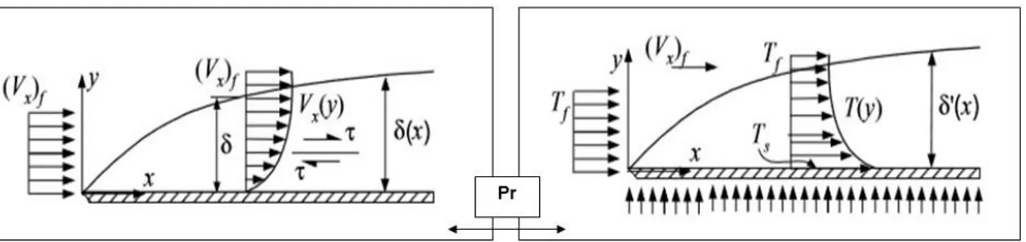
The convection heat transfer from a surface is function of the fluid motion over that, which is described by hydrodynamic boundary layer and thermal boundary layer. The development of the hydrodynamic boundary layer and the thermal boundary layer are related phenomena, described by the dimensionless Prandtl number (Pr) [2] (Eq. 7), whose simultaneous development greatly influences the temperature profile and thus the heat transfer by convection. Starting from the solution of the mass, momentum and energy transfer processes equations it is found that the Nusselt number can be express as a function of Reynolds number, that describes the hydrodynamic boundary layer and Prandtl number, link between the two boundary layers.
Figure 5: Hydrodynamic and thermal boundary layers for flow over a heated flat plate - Engineering Thermofluids - M. Massoud [2].
20
To demonstrate this relation between dimensionless numbers we consider a laminar flow over a flat isothermal plate and recall the definition of the convective heat transfer coefficient:
ℎ =
−𝑘𝑓𝑙𝑢𝑖𝑑∙ (𝜕𝑇𝜕𝑦)𝑦=0
(𝑇𝑤− 𝑇∞) [ W
m2∙ K] (13)
To explicitly express the term (𝜕𝑇
𝜕𝑦)𝑦=0, let's start recalling the governing equation for the
hydrodynamic boundary layer obtained from the conservation equation of momentum:
𝑉𝑥𝜕𝑉𝑥 𝜕𝑥 + 𝑉𝑦 𝜕𝑉𝑥 𝜕𝑦 = 𝑣 𝜕2𝑉 𝑥 𝜕𝑦2 (14)
and the governing equation for the temperature boundary layer obtained from the conservation equation of energy: 𝑉𝑥 𝜕𝑇 𝜕𝑥+ 𝑉𝑦 𝜕𝑇 𝜕𝑦 = 𝛼 𝜕2𝑇 𝜕𝑦2 (15) where 𝛼 = 𝑘 𝜌∙𝑐𝑝 [ m2
s ] is the thermal diffusivity. To find the analytical solutions of these
second-order, coupled partial differential equations we have to resolve them as a third order polynomials with the following boundary conditions. For the hydrodynamic boundary layer:
at y=0: vx=0 and 𝜕
2𝑉𝑥 𝜕𝑦2 = 0;
at y=δ: vx = 𝑣𝑓 and 𝜕𝑉𝑥
21
for the thermal boundary layer:
at y=0: T=𝑇𝑠 and 𝜕2𝑇 𝜕𝑦2 = 0; at y=δ′: T= 𝑇 𝑓 and 𝜕𝑇 𝜕𝑦= 0.
where δ is the hydrodynamic boundary layer and δ′ is the thermal boundary layer, 𝑣
𝑓 is the fluid
velocity, 𝑇𝑓 is the fluid temperature and 𝑇𝑠 is the surface temperature. Solving the third order polynomials applying these boundary conditions the velocity and temperature profile become:
𝑉𝑥 𝑉𝑓 = 3 2 𝑦 δ − 1 2( 𝑦 δ) 3 (16) and 𝑇 − 𝑇𝑠 𝑇𝑓− 𝑇𝑠 = 3 2 𝑦 δ′ − 1 2( 𝑦 δ′) 3 (17)
From the derivation of the conservation equations of mass, momentum and energy of the fluid entering and leaving a differential control volume by an integral approach, it is possible to find the relation between the hydrodynamic and thermal boundary layer function of Prandtl number (for the complete calculation see [2], chapter IVb, page 525-527):
𝛿′ 𝛿 = (
𝑃𝑟−1/3
1.026) (18)
Substituting Eq. 17 and Eq. 18 in the definition of the convective heat transfer coefficient, we find:
22 ℎ = −𝑘𝑓𝑙𝑢𝑖𝑑∙ (𝜕𝑇𝜕𝑦)𝑦=0 (𝑇𝑤− 𝑇∞) = 3 2 𝑘 𝛿′= 3 2 𝑘 𝛿(1.026𝑃𝑟 1 3) (19)
where we substituted for the thermal boundary layer thickness, δ′ in terms of the hydrodynamic
boundary layer thickness, δ. To show the relation also with the Reynolds number we have to remember that in case of flow over a flat plate in laminar conditions the hydrodynamic boundary layer is found to be (for the complete calculation see [2], chapter IVb, page 524-525):
𝛿 = 5𝑥 𝑅𝑒𝑥12 (20) Therefore: ℎ = −𝑘𝑓𝑙𝑢𝑖𝑑∙ (𝜕𝑇 𝜕𝑦)𝑦=0 (𝑇𝑤− 𝑇∞) =3 2 𝑘 𝛿(1.026𝑃𝑟 1 3) = 3 2∙ 𝑘 5𝑥𝑅𝑒 1 2(1.026𝑃𝑟 1 3) = 0.3 𝑘 𝑥 𝑅𝑒 1 2(𝑃𝑟 1 3) (21)
Using the definition of the Nusselt number we find:
𝑁𝑢 = 0.3 ∙ 𝑅𝑒𝑥12 ∙ 𝑃𝑟 1
3 𝑤𝑖𝑡ℎ 0.6 ≤ 𝑃𝑟 ≤ 50 (22)
This last expression demonstrate the dependency of the Nu number on Re and Pr numbers for laminar flow over a flat plate. A similar functional relationship for the Nu number is found also for a turbulent flow over a flat heated plate:
𝑁𝑢 = 0.0296 ∙ 𝑅𝑒45 ∙ 𝑃𝑟 1
23
Figure 6: Example of comparison of the Average Nusselt numbers as a function of the Reynolds number obtained for three tested micro-cells at 50 °C.
Therefore, in general we could express this relation as:
𝑁𝑢 = 𝐶 ∙ 𝑅𝑒𝑚 ∙ 𝑃𝑟𝑛 (24)
where constants C, m, and n depend on a specific case. In conclusion, being Nusselt number a measure of heat flux due to convection, the link with Reynolds number allows in first analysis to evaluate and compare the heat transfer properties of micro-cells at different flow rate conditions by means of the Nusselt-Reynolds diagram, as shown in Figure 6.
24
2.1 Friction factor and micro-cell efficiency
Being Nusselt number a measure of heat flux due to convection, the preliminary comparison of the micro-cells on the Nu-Re diagram allows to determine the geometry with higher heat exchange due to convective motions. However this does not take into account an important factor: the pressure losses along the channel. Thus, aiming to define an effective heat exchange efficiency parameter for each micro-device, pressure losses are evaluated in terms of the Fanning factor (𝑓). The Fanning friction factor is commonly assessed from experimental data as ([14],[20],[21]):
𝑓 = − ( 𝐷ℎ 0.5𝜌𝑈2) ×
∆𝑃
𝐿 (25)
the geometrical parameter 𝐷ℎ [m] and 𝐿 [m] are the hydraulic diameter and the channel length, respectively. The hydraulic diameter is defined as:
𝐷ℎ =
4𝐴𝑐
𝑝 (26)
with 𝐴𝑐 [m2] the channel cross-section area and 𝑝 [m] the wetted perimeter. While, the length 𝐿 is calculated for each geometry considering the channel middle line. ∆𝑃 [bar] is the inlet fluid relative pressure measured along the channel axial direction, measured by a pressure sensor on fluid delivery pipe. The ratio 𝐷ℎ/ 𝐿, shown in Table 1 for all geometries, together with the measured pressure values (∆𝑃) are the most influential parameters on the value assumed by 𝑓.
25
Table 1: 𝐷ℎ, L and 𝐷ℎ/ 𝐿 values for each micro-cell.
The term 𝑈2 [m
s] is the square flow bulk velocity determined as:
𝑈 =𝑄̇ 𝑆 [
m
s] (27)
Where 𝑄̇ [ml
min] is the volumetric flow rate and 𝑆 [m
2] is the channel section equal to 1 × 10⁻⁶ m2.
The density, 𝜌 [kg
m3], here function of fluid average bulk temperature, for water is calculated by
means of the physical model describing the density trend as a function of temperature [22]:
𝜌 = −0.003 ∙ 𝑇𝑏2− 0.042 ∙ 𝑇𝑏+ 1000 (28)
While for the two water-glycerin solutions the density values are calculated by online platform based on the formula of A. Volk and C.J. Kähler [23]. Once the pressure-drop losses are established on the base of the Fanning factor, 𝑓, the heat exchange efficiency of the micro devices, 𝜀 , is evaluated by dividing the mean Nusselt number by the Fanning friction factor, both dependent on Reynolds number, in accordance with Y. Sui et al. [14], W.M. Abed et al. [20], Z. Dai et al. [24]. Differently from mentioned literature, in our case the Nusselt and friction terms have not been normalized on a reference geometry, i.e. the straight channel.
Channel Type Channel length
L [mm] Dh [mm] Dh/L
Straight Channel 101 1 0.0099
Straight Parallel Channels type-II 101 2 0.0198
Standard Serpentine
(without and with ribs) 296.5 1 0.0034
26
𝜀 =𝑁𝑢̅̅̅̅(𝑅𝑒, 𝑃𝑟)
𝑓(𝑅𝑒) (29)
2.2 Entropy analysis
Following previous works on the argument ([25],[26]), another indicator of the local contribution to mixing and heat exchange is given by the local rate of entropy production, assuming convective motions without internal heat generation. Since any non-equilibrium process is an irreversible process, due to the second law of thermodynamics, it is possible to define the entropy production, S, as a function of temperature and velocity gradients. For this reason the third and last phase of the post-processing consist of to evaluate for each geometry the mean entropy production defined as:
𝑆 = 𝑘 𝑇02[( 𝜕𝑇 𝜕𝑥) 2 + (𝜕𝑇 𝜕𝑦) 2 ] + 𝜇(𝑇) 𝑇02 [2 {( 𝜕𝑢 𝜕𝑥) 2 + (𝜕𝑣 𝜕𝑦) 2 } + (𝜕𝑢 𝜕𝑦+ 𝜕𝑣 𝜕𝑥) 2 ] (30)
where 𝑇0 is the reference temperature of the system. In this study only the kinetic contribution is considered (second term right side of the equation).
In order to compare the micro-channels by mean fields (velocity magnitude, vorticity and entropy) and better appreciate the fluid motions differences induced along the channel paths, the velocity and entropy fields are normalized on bulk velocity, while the vorticity filed is normalized on the inverse of a single frame acquisition time. For a better comparison, also the reference axes have been normalized on the size of a single pixel, function of images resolution. The conversion factors from meter to pixel and from second to frame are determined starting by
27
the resolution and fps (frame/s) values set during the acquisitions. Examples are shown in the following table: Micro-cell Resolution [pixel] fps 𝐧° 𝐩𝐢𝐱𝐞𝐥 𝐦𝐦 𝟏 𝒇𝒑𝒔 [𝐬] [ 𝐩𝐢𝐱𝐞𝐥 𝐟𝐫𝐚𝐦𝐞] = 𝒙 ∙ [ 𝐦𝐦 𝐬 ]
Parallel Channels type-II 1024x880 5000 78 2 x 10⁻⁴ x = 0.0156
Standard Serpentine 1024x512 8500 81 1.2 x 10⁻⁴ x = 0.00972
Wavy-Sin. Serpentine 768x528 10000 92 1 x 10⁻⁴ x =0.0092
28
Chapter 3 - Materials and experimental methods
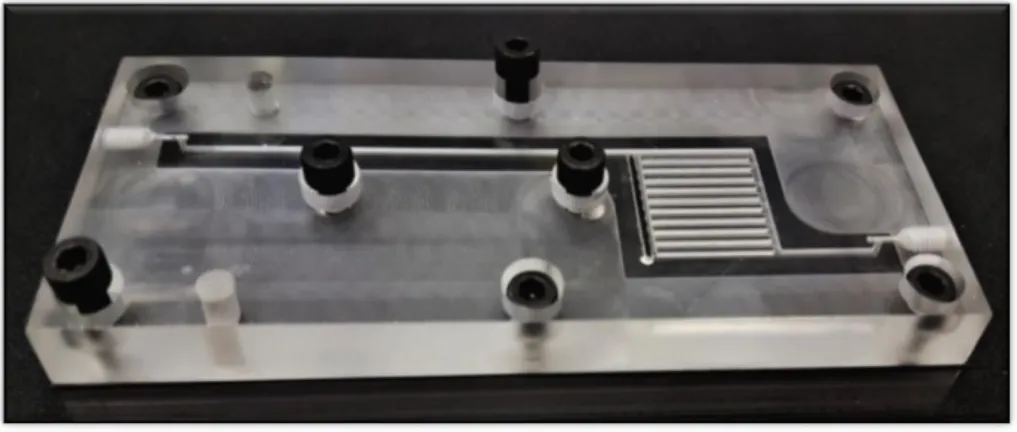
The setup, sketched in Figure 7, is designed to carry out temperature measurements and micro Particle Image Velocimetry (μPIV) measurements in order to investigate the thermal aspects and the fluid dynamics of the different micro-cell geometries and conditions tested in this work. The experimental setup is composed by:
o Thermal analysis • Hot Plate
• Thermocouple reader (accuracy: ±0.05 °C) • K-type thermocouples (accuracy: ±1 °C) • Infrared thermometer (accuracy: ±0.05 °C) • Syringe pump (accuracy: ±0.05 ml/min) o µPIV analysis
• Tracer (mean size 15 µm)
• Fastcam (pixel size 20 µm × 20 µm) o Pressure analysis
• Relative pressure sensor (accuracy: ±0.002 bar)
29
Starting from the first component to the left side of the scheme in Figure 7, the syringe Pump, Landgraff LA-800 (working range: 1.74 µL/hr to 340 ml/min, accuracy: ±0.05 ml/min), provided with a 140 ml syringe, introduces the cooling fluid into the micro-channel at different set flow rates. Distilled Water is used as the working fluid, but for the conventional serpentine path is also implemented a solution with two different percentages of glycerin and water (70 % glycerin and 30 % water; 30 % glycerin and 70 % water). The hot plate Stuart US-150 (working range: 0 °C to 325 °C), in direct contact with the micro-cell bottom side, is used to maintain the system under a constant heat flux setting up two temperature values equal to 50 and 70 °C, while four K-type thermocouples (working range: ±200 °C to +1372 °C, accuracy: ±1 °C) are used to measure the inlet/outlet water and the micro-cell surface temperatures. To carry out μPIV measurements the micro-cell is placed under a high-speed camera Photron Mini AX100 (working range: 5000 fps (frames/s) at resolution of 1024 × 880 pixel, up to 12500 fps at 640 × 480 pixel, accuracy: pixel size 20µm × 20µm) to acquire high resolution images of the region of interest and the working fluid is seeded by hollow glass spherical tracers Sphericel 110P8with mean size equal to 15 µm provided by Potters Industries LLC. In order to evaluate the heat exchange efficiency for each geometry, the pressure drop (ΔP) along the axial direction of the microchannel is measured by a Flowplus16-ViscoTec relative pressure sensor (working range: 70 mbar to 7 bar, accuracy: ±0.002 bar). For each instrument more details will be provided in the following paragraphs.
3.1 Micro Devices
Six different geometric configurations are used for laboratory testing: the classical straight channel configuration, the two configurations with parallel channels (named in Figure 8 as type-I and type-II), the conventional serpentine path, with and without ribs, and the wavy-sinusoidal serpentine path.
30
Figure 8: Geometrical configurations studied.
All micro-devices are composed of an aluminum bottom side and a plexiglass top side. The micro channel is milled on the adiabatic part of the micro-cell to help cooling by micro heat exchangers application on existing industrial devices. To assess the influence of the channel material on the heat exchange rate, a comparison between the straight parallel channels cell type-I assembled in an adiabatic material (plexiglass) and assembled in a conductive material (aluminum) was also carried out. The overall structure of the cells has a total length of 120 mm, a width of 50 mm and a height of 22 mm. In particular, for all the cells the plexiglass top side has a height of 10 mm, while the aluminium bottom side is slightly higher, i.e. equal to 12 mm to allow the insertion of the thermocouples. The upper and lower parts are tightened together by M4 type screws. The tested geometries are manufactured in the mechanical workshop of the Department of
31
Mechanical and Aerospace Engineering (DIMA) of University La Sapienza. The processes are performed by numerically controlled milling machine (CNC) on the base of detailed CAD drawings of the single parts to be realized. The use of a CNC milling machine allowed to obtain the channel path with a precision of about ±0.01 mm. To avoid leakage of cooling fluid and to guarantee a pressure sealing, all configurations have three common elements. The first concerns the realization of a 2 mm wide frame around the channel path, as shown in Figure 9.
Figure 9: Example of a sealing frame manufactured on the straight parallel channels cell type-I.
32
Figure 11: Inlet and exit tubes.
The second is the insertion of a black neoprene gap-pad (for PIV measurements, to enhance the particle tracer images over background) or an aluminum gap-pad (for thermal measurements, to guarantee heat transfer), with a thickness of about 1 mm, between the top and bottom side of the cell. An example of cell assembly with gap-pad is shown in Figure 10. Thirdly, to connect the micro-cell to the syringe pump, a PVC tube with an internal diameter of 1.2 mm and a special Luer-Lock connection is used. The PVC tube is joined to another PLA tube with an internal diameter of 1 mm that is inserted directly in the cell and fixed with a perforated screw. An additional rubber gasket located at the PLA tube outlet section prevents leaks at the inlet of the channel. For the exit tube, internal diameter 1 mm, seal is guaranteed only by rubber gasket located at the connection point between the outlet section of the channel and the tube inlet section. The 300 mm long inlet tube and the 100 mm long exit tube are shown in the following Figure 11.
33
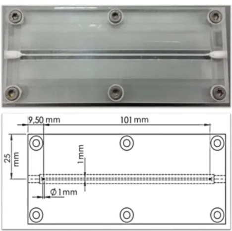
3.1.1 Straight channel micro-cell
The cell used for the validation of the measurement system consists of a simple straight channel milled on the plexiglass top. The duct has a square cross-section 1 × 1 mm2, a length of about
101 mm and a heat exchange area equal to 101 mm2. The main features of the straight channel
are reported in Table 3.
Figure 12: Top view and CAD drawing of the straight channel micro-cell.
Channel length [mm] 101
Hydraulic diameter [mm] 1
Heat exchange area [mm2] 101
Plexiglass top thickness [mm] 10
Aluminium base thickness [mm] 12
34
Figure 13: View of the aluminum bottom side and CAD drawing of the thermocouples venues.
As shown in Figure 13, the aluminum bottom side of the micro-cell presents in the sidewall three holes for the positioning of the thermocouples in order to measure the surface temperature. The three holes have a variable diameter of 2 mm up to a depth of 20.50 mm and of 1 mm in the last 5 mm (Figure 13). The three thermocouples are located at the middle of the channel, distant 9 mm one from each other and at a depth of 0.5 mm.
3.1.2 Straight parallel channels micro-cell type-I
The cell is made as a prototype of a parallel channels micro-heat exchanger to study the flow distribution in each (single) channel. Possible changes to be made to increase the homogeneity of the flow within all channels have been considered and applied in the straight parallel channels micro-cell type-II. The starting geometry, shown in Figure 14, is composed of 11 parallel channels with a square cross-section 1 × 1 mm2, an inlet aligned with the first channel and an
35
outlet duct aligned with the last one. Only the vertical manifold, downstream of the inlet channel, has a cross-section 2 × 1 mm2 in order to insert elements to guide the fluid in the channels
(Figure 15). This configuration has a heat exchange area around 308 mm2 and a distance
between the entrance and exit hole of about 101 mm. As reported in Table 4 the inlet channel length is around 65.5 mm to allow a complete development of the velocity field in laminar regime. This length is established on the base of the following definition [2],[18]:
𝐿𝑖𝑛𝑙𝑒𝑡 = 0,05 ∙ 𝐷ℎ∙ 𝑅𝑒 (31)
Where 𝐷ℎ the hydraulic diameter. By considering a hydraulic diameter equal to 1 mm and a flow rate of 78 ml/min (Re = 1300) the inlet length needed for a complete development of the velocity field is equal to 65 mm.
Total Channel length [mm] 101
Single Channel length [mm] 17
Inlet Channel length [mm] 65.5
Outlet Channel length [mm] 13.5
Hydraulic diameter [mm] 1
Heat exchange area [mm2] 308
Plexiglass top thickness [mm] 10
Aluminium base thickness [mm] 12
36
Figure 14: Top view and CAD drawing of the straight parallel channels micro-cell type-I.
The fluid guide elements, made by laser cutting technology due to the very small dimensions, were designed with well-studied shapes based on a preliminary study [27] able to better distribute the flow rate along the different channels. The Figure 15 shows the four profiles manufactured.
37
Figure 16: Top view of the aluminum straight parallel channels micro-cell type-I.
Unlike the other configurations, for this cell, the thermocouple holes in the aluminum bottom side have not been made, since the study was focused especially on the analysis of the flow distribution inside the channels. In addition, to evaluate the influence of the channel material on the heat exchange rate, this configuration is the only one that was assembled also in a conductive material (aluminum) and compared with the plexiglass one on the base of the fluid outlet temperature. In Figure 16 the aluminum straight parallel channels micro-cell type-I is shown, the geometric features are the same as the previous one, except for a major heat exchange area equal to 775 mm2.
3.1.3 Straight parallel channels micro-cell type-II
The type-II parallel channels cell, to be considered as a reference for the study, is designed as an evolution of the previously described geometry. The study of the flow distribution in the cell type-I suggested the modification of the inlet and outlet ducts geometry from the parallel channels section and critical points such as leading edges between fluid and ribs. In detail, as shown in Figure 17, the inlet and outlet ducts have been transformed into flow collection areas, symmetrical with respect to the parallel channels section, with a curvilinear profile (angles equal
38
to 16° and 31°) and growing cross-section (from 1 mm to 21 mm). In order to prevent preferential flows in the central ducts, balance the inlet and outlet pressure gradient and guide the flow towards peripheral channels. The critical points as leading edges between fluid and ribs have been rounded to avoid flow separation and generation of three-dimensional motions. The test section is composed by 11 square cross-section 1 × 1 mm2 channels and has the same size of
the previous one, 19 mm × 21 mm. The heat exchange area is around 947 mm2 with a distance
between the entrance and exit hole of about 101 mm.
Total Channel length [mm] 101
Single Channel length [mm] 19
Hydraulic diameter [mm] 2
Heat exchange area [mm2] 947
Plexiglass top thickness [mm] 10
Aluminium base thickness [mm] 12
Table 5: Main features of the straight parallel channels micro-cell type-I.
39
Figure 18: View of the aluminum bottom side and CAD drawing of the thermocouples venues.
Also in the aluminum bottom side of this geometry there are three thermocouples venues, but, differently by the straight channel, two venues are located in the right sidewall and one in the left wall in order to measure the surface temperature under the two most peripheral channels and under the central one. As shown in Figure 18, the three holes have different lengths and also in this case the diameter varies with depth.
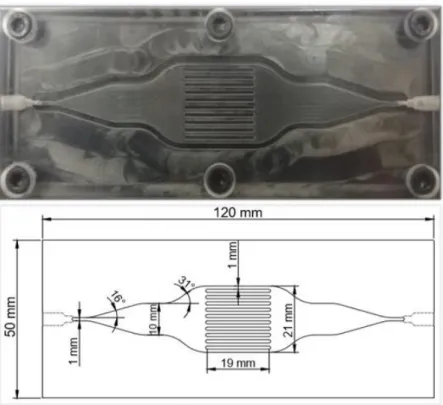
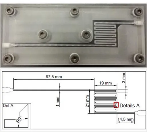
3.1.4 Standard serpentine micro-cell
A standard serpentine cell is implemented to test this well-known configuration in a different adiabatic material, in view of an easy implementation on existing engineering devices. The channel of the standard serpentine configuration has a square cross-section 1 × 1 mm2, an
40
characterized by 11 U-elements. Each U-element of the geometry has two horizontal sections with a length of 19 mm and a vertical section with a length of 3 mm. The test section is 19 mm × 21 mm, while the heat exchange area is 296.5 mm2. The main features are reported in Table 6.
Total Channel length [mm] 296,5
Single Channel length [mm] 19
Inlet Channel length [mm] 67,5
Outlet Channel length [mm] 14,5
Hydraulic diameter [mm] 1
Heat exchange area [mm2] 296,5
Plexiglass top thickness [mm] 10
Aluminium base thickness [mm] 12
Table 6: Main features of the standard serpentine cell.
41
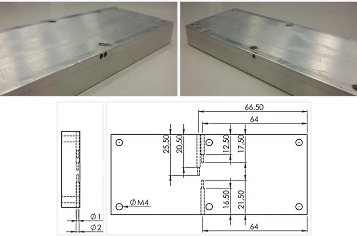
For the standard serpentine and wavy-sinusoidal serpentine cells the aluminum base has the same characteristics. Unlike the previous cells, in these last cases, the holes for thermocouples are located on the short side of the base so as to measure the surface temperature under the first channel, the last channel and the central one (Figure 20). The three venues have a variable diameter of 2 mm up to a depth of 27.50 mm and of 1 mm in the last 5 mm of depth (Figure 20). The three thermocouples are located at the middle of the channel, distant 10 mm from each and at a depth of 0.5 mm. This configuration is also tested with horizontal ribs, the goal being to increase the device efficiency by a higher heat exchange surface, without altering the main features of the geometry, using conductive elements inside the channel (ribs). The new heat exchange area is equal to 459.3 mm2. The ribs are cylindrical steel elements with a diameter of
0.4 mm and a length of 17 mm equal to the single channel length; they are fixed on the gap-pad surface in alignment whit the duct axis and positioned in the middle of the channel, Figure 21a. The view of the cross-section in Figure 21b shows the reduction of flow passage in the U-element horizontal sections from a square cross-section 1 × 1 mm to two side aisles 0.3 mm × 1 mm and one upper section 1 mm × 0.6 mm.
42
Figure 21: Standard serpentine micro-cell with ribs. (a) Top view of the test section; (b) View in the cross-section with rib.
3.1.5 Wavy-sinusoidal serpentine micro-cell
This geometry was designed to increase the thermal exchange efficiency without addition of elements inside the channel, e.g. ribs, due to possible limitations in the modification of mechanical or electrical components to be cooled and to large pressure losses. The aim is to obtain a higher heat exchange rate through a wavy geometry to increase the wetted surface and promoting the generation of three-dimensional motions. The idea is to combine the fluid mixing properties of the wavy path [24] with the heat transfer properties of the standard serpentine path [28], leading to the realization of a new wavy-sinusoidal serpentine micro-cell, shown in Figure 22.
The new proposed channel has a square cross-section 1 × 1 mm2 and an equivalent length of 354
mm. The test section has the same size of the standard serpentine and parallel channels configurations equal to 19 mm × 21 mm. As the previous cell, the inlet channel length of 67 mm allows a complete development of the thermal and velocity fields. Each wavy element has an
43
inner radius of 0.25 mm and an external radius of 1.25 mm. This configuration is characterized by 7 U-elements with two horizontal sections with a length of 19 mm and a vertical section with a length of 5.6 mm. The aluminium base is the same of the standard serpentine cell.
Total Channel length [mm] 354
Single Channel length [mm] 19
Inlet Channel length [mm] 67.5
Outlet Channel length [mm] 14.5
Hydraulic diameter [mm] 1
inner radius [mm] 0.25
external radius [mm] 1.25
Heat exchange area [mm2] 354
Plexiglass top thickness [mm] 10
Aluminium base thickness [mm] 12
Table 7: Main features of the wavy-sinusoidal serpentine cell.
44
3.2 Syringe Pump
Figure 23: Hll Landgraf LA-800 Syring Pump.
The syringe pump used is an Hll Landgraf LA-800. This analogue instrument allows to work with 140 ml syringes and up to a 12 bar pressure. From the LCD/LED display it is possible to set:
• The Rate: from a minimum of 1.74 µL/ hr to a maximum of 340 ml/min; • the volume of the syringe: in our case equal to 140 ml;
• the diameter of the syringe: in our case equal to 40 mm.
Through the pump controls positioned below the display is possible to set a flow rate in ml/min with a single digit after the decimal point, which corresponds to an instrument absolute error on our flow rate settings equal to ±0.05 ml/min. For the experimental tests it was necessary to modify the supplied plastic syringe and make another special one in aluminum. This was done to increase its structural resistance, in order to withstand the considerable stresses given by the thrust forces exerted by the pump on the syringe piston due to the high fluid entry pressure in the micro-cell. Especially in case of very complex geometries, e.g. wavy-sinusoidal serpentine, or
45
Figure 24: Modified 140 ml aluminum syringe. Lateral view (left image) and front view (right image).
very viscous cooling fluid, i.e. glycerin. The modified 140 ml syringe, shown in Figure 24, is reinforced with an outer extruded aluminum sleeve and the plastic piston is completely replaced by a solid aluminum cylinder on which the rubber sealing cover can be fixed.
3.2.1 Flow rate studied
As briefly said before, the micro-cell geometry and the type of fluid to be used greatly influence the thrust force that the syringe pump exerts on the fluid into the micro-device. The thrust also depends on the set flow rate and therefore on the flow regime in the channel, e.g. laminar, transient, turbulent. For this reason, it was not possible to define a number of equal flow rates for all configurations, since for some of these the thrust required to introduce the fluid into the channel far exceeded the mechanical limits of the instrument (Maximum operating pressure: 12 bar; maximum operating force: 100 kg). The flow rates considered to perform the thermal measurements are reported in the following table for all configurations. To carry out μPIV measurements, the flow rates of 30 ml/min and 90 ml/min were considered for all cells.