UNIVERSITA' DI BOLOGNA
SCUOLA DI SCIENZE
Corso di Laurea Magistrale in BIOLOGIA MARINA
Are there genetic breaks between Atlantic and Pacific Yellowfin tuna (Thunnus albacares) populations?
A preliminary study based on microsatellites gene variation
Tesi di laurea in Struttura e connettività delle popolazioni marine
Relatore Presentata da
Prof. Fausto Tinti Manuel Umberto Romeo
Correlatori
Dott. ssa Ilaria Guarniero Dott. Carlo Pecoraro Dott. ssa Alessia Cariani
III sessione
INDEX
Abstract
1. Introduction ... 1
1.1 Yellowfin Tuna biology and ecology ... 1
1.2 Tropical tuna fisheries ... 3
1.2.1 FAD-based fishery ... 5
1.3 Discrimination of Juvenile Yellowfin ... 7
1.4 YFT population structure and current management ... 10
2. Aim of the study ... 13
3. Materials and Methods ... 14
3.1 Sampling design ... 14
3.2 DNA extractions ... 16
3.3 Species identification (ATCO barcoding) ... 17
3.4 Microsatellites loci and genotyping ... 19
3.6 Binning ... 21
3.7 Microsatellite dataset analysis ... 22
5. Results ... 25
5.1 ATCO barcoding ... 25
5.2 Genetic differences between Pacific and Atlantic specimens. 27
6. Discussions and conclusions ... 37
6.1 Species identification for YFT juveniles ... 37
6.2 Yellowfin tuna population structure and possible implications
for its management ... 39
7. References ... 43
Appendix A - ... 53
Abstract
Yellowfin tuna (Thunnus albacares, YFT, Bonnaterre 1788) is one of the most important market tuna species in the world.The high mortality of juveniles is in part caused by their bycatch. Indeed, if unregulated, it could permanently destabilize stocks health. For this reason investigating and better knowing the stockboundaries represent a crucial concern. Aim of this thesis was to preliminary investigate the YFT population structure within and between Atlantic and Pacific Oceans through the analysis of genetic variation at eight microsatellite loci and assess the occurrence of barriers to the gene flow between Oceans. For this propouse we collected 4 geographical samples coming from Atlantic and Pacific Ocean and selected a panel of 8 microsatellites loci developped by Antoni et al., (2014). Samples 71-2-Y and 77-2-Y, came from rispectively west central pacific ocean (WCPO) and east central pacific ocean (ECPO), instead samples 41-1-Y and 34-2-Y derive from west central atlantic ocean (WCAO) and east central atlantic ocean (ECAO). Total 160 specimens were analyzed (40 per sample) and were carried out several genetic information as allele frequencies, allele number, allelic richness, HWE (using He and Ho) and pairwise Fst genetic distance.
Results obtained, maysupport the panmictic theory of this species, only one of pairwise Fst obtained is statistically significant (Fst= 0.00927; pV= 0.00218) between 41-1-Y and 71-2-Y samples. Results suggest low genetic differentiation and consequent high level of gene flow between Atlantic and Pacific populations.
Furthermore, we performed an analysis of molecular taxonomy through the use of ATCO (the flaking region between ATPse6 and cytochrome oxidase subunit III genes mt DNA, to discriminate within the gener Thunnus two of the related species (Yellofin and bigeye tuna) according with their difficult recognition at certain size (<40 cm).
ATCO analysis in this thesis, has provided strong discriminate evidence between the target species proving to be one of the most reliable genetic tools capable to indagate within the genus Thunnus. Thus, our study has provided useful information for possible use of this protocol for conservation plans and management of this fish stocks.
1
1. Introduction
1.1 Yellowfin Tuna biology and ecology
YELLOWFIN TUNA
Order - Perciformes Family - Scombridae Genus - Thunnus Species - albacares
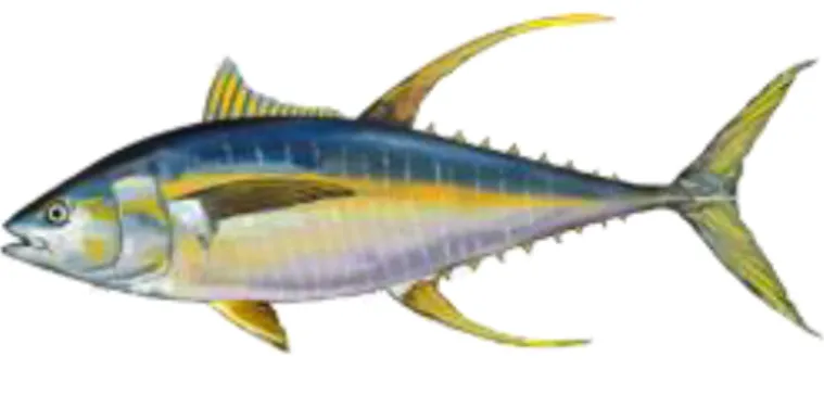
Yellowfin tuna (Thunnus albacares, YFT, Bonnaterre 1788) (Fig. 1) is a pelagic fish widely distributed in tropical and subtropical waters worldwide (Fig. 2). It is one of the most important market tuna species in the world and it is fished in the Indian, Pacific, and Atlantic Oceans, where it has been commercially harvested since the early 1950s (Collette and Nauen, 1983; Miyake et al., 2010).
YFT are torpedo-shaped fish with about 20 broken vertical lines in the belly and a typical dark blue colour on the back and upper sides. They have very long anal and dorsal fins that are bright yellow, from which their common name is derived (Collette and Nauen, 1983). YFT are relatively fast growing, and they can grow up to 200 cm FL and 175 kg with a life span of about 8 years (ISSF 2013).
Tagging experiments indicate that YFT adults are able to undertake wide migrations, according to the fact that they are fairly fast swimming and highly migratory fishes (Schaefer, 2007). Although their potential for trans-oceanic’s migrations, the majority of tagged individuals are recovered within several hundred kilometres from their release positions (Schaefer, 2008). YFT usually spend most of their life in the warmest first 30-40 meters of the water column (Block, 1997). This behaviour seems to be strictly related to the reproductive biology of this species, as reviewed by Schaefer (2001) spawning events,
2
as for other tuna species, can occur in relation to the sea surface temperature over 24ºC. YFT is a batch-spawner characterized by an asynchronous ovary organization (Schaefer, 2001) and an indeterminate fecundity (Zudaire et al., 2013). YFT can spawn with a frequency of approximately 1.52 days (McPherson, 1991; Schaefer, 2001), throughout the year (Itano, 2001; Stéquert et al., 2001). Moreover, sea surface temperature deviations from 24°C could seriously decrease their potential spawning activity (Itano, 2001).
Worldwide studies on the fork length at which 50% of females reach maturation (L50) provide different estimates among oceans and areas. For example, in the Indian Ocean L50 was estimated around 100 cm FL (Zhu et al., 2008), McPherson (1991) estimated it as 108 cm FL in the western Pacific Ocean, while Schaefer (1998) estimated this parameter as 92 cm FL in the eastern Pacific Ocean, and Itano (2001) reported a L50 of 104 cm FL for the equatorial west Pacific. In all these studies, the L50 was defined with macroscopic method by setting maturity limit in advanced vitellogenic ovaries (Itano 2001). Instead, Zudaire et
al., (2013) in Indian Ocean, applied a maturity threshold in ovaries in Cortical Alveoli
(CA) stage, retrieving a L50 value of 75 cm FL. CA stage represents the earliest sign of oocyte maturation (Murua and Motos, 2000), and females in this developmental stage usually go through vitellogenesis and spawn in the upcoming season (Wright, 2007). During the reproduction, YFTs continue feeding, and its spawning activity has been described to be dependent on the prey availability (Itano, 2001). Thus, they need energy from feeding to carry out ovarian development (Zudaire et al., 2013), and for this reason the species could be described as a capital-income breeder (Alonso-Fernández and Saborido-Rey, 2012). According to this strategy, fishes require energy from feeding, because the energy stored before reproduction is not enough to offset a successful reproduction (Henderson and Morgan, 2002).
YFT diet includes variable prey composition. Poitier et al., (2007), studying the stomach contents of YFT caught by long-line fishery in Indian Ocean, indicated fishes as their main food source, while for YFT caught by Atlantic purse seine fisheries the favourite nutritional resources seem to be mainly small pelagic fishes (Menard and Marchal, 2003). In addition, there are significant differences in prey species composition for the specimens captured around fish aggregating devices (FAD) and free-swimming schools (FSC). Stomach-contents analyses have indicated Vinciguerria nimbaria (Photichthyidae, philum Chordata) as the main food source in FAD-associated small YFT, whereas small little
3
Scombridae, mixed with Cubicepspauci radiatus (Nomeidae, philum Chordata) are the main preys in YFT FSC-associated school (Dagorn et al., 2007).
Besides these data, the percentage of empty stomachs found in YFT FAD-associated (85%) is higher than those caught on unassociated schools (25%), underlying the possibility that these fish do not feed under drifting FADs (Menard et al., 2000).
Fig. 2_Yellowfin geographical distribution.
1.2 Tropical tuna fisheries
Tuna fisheries operate on an industrial scale in the Indian, Atlantic and Pacific Oceans (Davies et al., 2012), representing more than 4.1 million tons of the global fisheries catches and are dominated by three fishing gears, i.e. purse-seine, longline, and pole and line, accounting for about 60%, 15% and 11% of the world tuna catches respectively (FAO, 2012).
The European tuna purse-seine fishery targets yellowfin (Thunnus albacares), skipjack (Katsuwonus pelamis), and bigeye (Thunnus obesus) tuna since the early 1980s (Amandè
et al., 2012).
European purse-seine fishery total catches of the principal commercially tuna species have achieved a maximum of about 400 000 t in 2003 and have fluctuated around 250 000 t in
4
recent years (Pianet et al., 2010). This fishing method implies that the fish are pursued and encircled by vessels of a broad range of sizes and capacities (Fig. 3). The net employed has a length that may reach more than 2200 m and its depths are usually from 150 m to 350 m; the mesh size varies from 7.5 cm to 25 cm but the vast majority is employing a 10.8 cm stretched mesh (FAO, 2012).
Fig. 3_Purse seiner fishing activity
Tropical tuna purse seine fishery is characterized by two fishing modes with sets made on: 1) tuna schools associated with floating objects (FADs - Fishing aggregating device) and 2) on free schools (FSC - Free swimming schools) (Amandè et al., 2010).
FSC can be detected from signs on the surface of the water, in fact schools usually move close to the surface while chasing. Frequently, the presence of birds close to the surface (blackspot), is a further hint for the presence of free tuna schools (Allen, 2010).
5
Fig. 4_Free schools catch during landing procedures.
Instead, FAD sets are generally less mobile than FSC sets, making their catch easier. FAD could be natural objects or man-made (raft or plastic), with a long net below and can be either anchored (aFADs) or drifted (dFADs) depending on the fishing area (Dagorn, 2011). FADs are easier detectable than FSC, decreasing sighting effort and time required to locate fish schools. (Dempster and Taquet, 2004). The main difference between the two fishing methods is their target; in fact FSC's target is represented by large YFT (Fig. 4) and bigeye tuna (e.g. up to 100 cm FL), instead FAD sets focus on catching adult skipjack tuna (Dagorn et al., 2013).
1.2.1 FAD-based fishery
Tropical tuna purse seine fisheries have globally increased their use of drifting fish aggregating devices (dFADs) since the early 1990s, in order to improve catch levels (Dempster and Taquet, 2004; Dagorn et al., 2013). In fact sets around FADs have shown higher achievement rate (90%), compared with the FSC (50%) (Fonteneau et al., 2000). In addition, in the last years, FAD-based fishery has recorded an impressive technological development, (e.g. echo-sounder, GPS units attached to their buoys) that allow to the fishermen to know their movements and to track their routes, but also to know the fish
6
composition and abundance below them (Lopez et al., 2014). In this context, in the last years almost half of all principal market tunas were caught by sets on dFADs, of which an estimated 50,000–100,000 are deployed each year (Baske et al., 2012).
The loss of potential yield and the reduction of spawning stock biomass (SSB) can be some of the ecological and biological problems linked to the constant and unchecked increase in the use of FADs (Fig. 5) (Fonteneau and Ariz, 2011).
Dagorn et al., (2012) showed that the total harvested target species associated with dFADs, are composed for 75% by adults SKY. While the by-catch of juvenile BET and YFT (40-65 cm FL) (Fonteneau et al., 2000, Bromhead et al., 2003) inadvertently caught with this fishing gear, counts respectively for 16% and 9% of the global tuna catches. By-catch can be defined as accidental catches, which are not the target of the specific fishing method employed, representing a widespread environmental problem (Hall, 2000). However, accurate data on it are of essential importance for the stock assessment of these species, but currently data are still poor or even unreported, due to the fact that most of juvenile tuna by-caught are discarded or sold at local markets (Romagny et al., 2000).
YFT can grow to sizes that are much larger than those typically caught with FAD sets. The potential yield of YFT population would be much higher if the harvest of small fish will be reduced, improving their status and mitigating the current overfishing (ISSF, 2012).
Fig. 5_Underwater drifting FADs nets.
In addition, juveniles overfishing, as well as adults overfishing, might reduce the spawning stock biomass (SSB) or bring stocks under the Maximum Sustainable Yield (MSY). For instance, Pacific and Atlantic Ocean stocks that are experiencing high fishing mortality seem to display similar value below the SSBMSY (Dagorn et al., 2013).
7
FAD-based fishery could also affect tropical tuna ecology and behaviour, driving fishes in areas probably not advantageous for their feeding; constituting what is described as "Ecological Trap", leading fishes in poor-quality habitats (Marsac et al., 2000). In this scenario, population productivity could be reduced as a consequence of maladaptive habitat choice (Schlaepfer et al. 2002). On the contrary, natural floating rubble, usually tend to be accumulated in confluent areas, with high nutrients and forage rate (Bromhead
et al., 2003). Thus, in general these animals would follow the movement of the natural log
to feed, but due to the increasing presence of dFADs in the sea, they are forced into different areas (Marsac et al., 2000).
Finally floating objects can also impact coastal ecosystems when hit by waves and crashed up on coral reefs, causing physical damages on corals (Dagorn et al. 2013).
1.3 Discrimination of Juvenile Yellowfin
Among the different species caught accidentally around FADs, small and immature tropical tunas represent the largest group in terms of number of individuals (Amandè et al., 2010). For instance, in Atlantic Ocean the number of tuna juveniles caught as by-catch, between 2003 and 2007, was estimated in 751.000 individuals (Amandè et al., 2010), and most of them were thrown back to the sea (dead or alive), or were traded in local markets (Romagny et al., 2000).
It appears clear how further researches in this field are necessary, to improve scientific knowledge on the growth and natural mortality of juvenile tunas, in order to understand the real impact of the FAD-based fishery on the ecology and biology of these species (Bromhead et al., 2003).
Although adult BET and YFT present different external characteristics which allow easy discrimination (e.g., eyes diameter, body coloration, marks) these differences are less evident when the specimens are below a certain size (<40 cm FL) and even more when specimens are frozen (Fig. 6). Furthermore, species misidentification at their post-larval and early-stage juveniles could be caused by geographical variation in their morphological features (Chow and Inoue, 1993).
8
Fig. 6_juveniles yellowfin (left) and bigeye (right)
Thus, very high-quality taxonomic skills are required to discriminate between them, in fact it has been underlined that misidentification by fishery-data collectors can be as high as 30% (Chow and Inoue, 1993). An important internal characteristic that allows to discriminate between the two species is the liver morphology (Itano, 2004): asymmetric for YFT without striations vs. symmetric for BET with surface striated (Fig. 7). However during sampling activities is not always possible to work with the whole fish, vanishing any possibility to identify these species using this internal character.
Fig. 7_liver morphology
The specific identification of these tuna is fundamental to improve data about their catches and distribution and provide more accurate information on the real mortality of juveniles
9
that affects negatively their yield per recruit. Among the different methodologies developed to overcome misidentification issues, DNA-based identification methods represent a very accurate and precise tool because DNA can be extracted by almost all types of samples (fresh, frozen, canned, dried tissues) (Teletchea et al., 2009). Many different DNA markers have been used for tuna and tuna-like species identification, but the analysis of the mtDNA regions, both using restriction endonucleases or through the nucleotide sequence analysis, is the preferred method to identify individuals (Billington and Hebert, 1991).
However, a specific gene marker has to be selected appropriately and detailed knowledge of the DNA sequences from target species is required before setting-up the methodology and validate the final assignation, otherwise species misidentification can occur, especially when within-species and between-species genetic distance are of similar magnitude (Chow et al., 2006).
Different gene regions in mitochondrial DNA or in nuclear DNA have been proven more useful than other to discriminate among these species. For instance the restriction fragment length polymorphism (RFLP) analysis using the cytochrome b (cytb) and 12s RNA (12Sr) gene fragments failed in the attempt to discriminate between tuna (Chow and Inoue, 1993). Instead a possible rapid molecular instrument to the discrimination between different individual is the multiplex-based PCR.
In fact, few multiplex-based analysis were tested to discriminate between different species (i.e, Thunnus thynnus from Sarda sarda, Lockley and Bardsley, 2000); Michelini et al., (2007) tested a triplex-polymerase chain reaction of the ctyb sequences to discriminate between three tuna species, with successful result.
However, using restriction endonucleases or nucleotide sequence analysis, the flaking region between ATPse6 and cytochrome oxidase subunit III genes (ATCO) was verified as one of the most performing marker in discriminating the eight tuna species (Chow and Inoue 1993).
Hebert et al., (2003) suggested the use of 648 base pair (bp) portion of the mitochondrial DNA gene cytochrome oxidase subunit I (cox1) as universal marker to differentiate a vast spectrum of animal species (DNA barcoding). Therefore, COI has been commonly used for discriminating among fish species, including tuna and tuna-like species, even if many issues have been pointed out in using a single genetic marker for all fish species (Ward et
10
al., 2005). Moreover, Alvarado-Bremer et al., (1997) have underlined as the mtDNA Control Region (CR) is not capable to detect differences between related species of the genus Thunnus.
Thus, Chow et al., (2006) detected no evidence of genetic differences between BET and YFT, through the use of the nuclear genetic marker ITS1 (nuclear fragment rDNA first internal transcribed spacer).
Instead, Vinas and Tudela, (2009) employing a combined approach between this marker together with the mitochondrial genetic marker CR have shown promising results in discriminating the 8 species of Thunnus in general, and YFT and BET in particular.
1.4 YFT population structure and current management
The International Union for Conservation of Nature (IUCN) classify YFT as NearTreatened at the global scale, underlining the importance of taking urgent management
measures for the conservation of this species to avoid any possibility of populations collapse. Moreover, the Convention on the Law of the Sea (2012) has classified YFT as highly migratory species in its Annex I, underlying how the nations should cooperate in its conservation.
The monitoring and management of YFT populations, as for all tuna and tuna-like species, are under the jurisdiction of four independent Regional Fisheries Management Organizations (RFMOs) (Fig. 8). The West and Central Pacific Fisheries Commission (WCPFC), the Inter-American Tropical Tuna Commission (IATTC), the International Commission for the Conservation of Atlantic Tuna (ICCAT) and the Indian Ocean Tuna Commission (IOTC).
11
Fig. 8_Tuna worldwide RFMOs
The life-history traits of this species, such as their high mobility and dispersal capacity, extraordinary fecundity and large population sizes, have reduced the possibilities to discriminate clearly its stocks boundaries, leading to consider panmitic populations within each ocean. In fact YFT populations are actually monitored and managed independently by each of the four RFMOs, and management strategies and models often lie on stock assessments that are systematically distorted by insufficient fishery and population biology data.
Understanding the spatial structure of YFT populations is a central key to the assessment and management of these economically and socially important species. The first attempt to delineate YFT stock structure date back to Suzuki (1962), using TG2 blood group antigen in samples of Pacific and the Indian Oceans, which showed no differences between samples.
Many other genetic studies employing both mtDNA and nDNA markers have been conducted to investigate yellowfin population structure. Ward et al., (1994), failed in identifying possible local structuring within the Pacific Ocean using five allozymes. Instead Appleyard et al., (2001), analysed samples from the central / western Pacific Ocean and the eastern Pacific Ocean, employing 5 microsatellite loci (SSRs - simple sequence repeats). Their study showed significant heterogeneity at one of five microsatellite loci
12
analyzed, although not enough differentiation to prove the presence of multiple stocks within the Pacific Ocean.
Similar results have been showed by Diaz-Jaimes and Uribe-Alcocer, (2006), through the analysis of seven different SSR loci. They did not detect any signs of differentiation within the Pacific Ocean confirming the absence of YFT local partitioning.
The first worldwide genetic study on YFT population structure was made by Ely et al., (2005), using the mtDNA control region CR. Their results present very low differentiation, suggesting the presence of a single large panmictic population at the global scale. However, recent genetic studies in Indian Ocean have suggested that YFT could have a more fragmented population structure than what assumed in its assessment and management process so date. Dammannagoda et al., (2008), suggested the possibility that genetically discrete yellowfin tuna local sub-populations may be present in the north western Indian Ocean, detecting significant genetic differentiation among sites for mitochondrial DNA (Φst = 0.1285, P <0.001) and at two microsatellite loci (Fst = 0.0164, P <0.001 and Fst = 0.0064, P <0.001). This issue has been also corroborated by Swaraj et
al., (2013) with the proposed presence of at least three genetic stocks of YFT in Indian
waters.
These discordant information underline the need to dig deeper into the YFT stock structure, according to the fact that if the stock assessment and management rely on invalid assumptions, there will be a failure of the conservation and the optimal economic use of this resource. Thus, if populations are distinct, some of them could locally collapse and management measures might focus on the wrong populations.
13
2. Aim of the study
This thesis was developed within the framework of an ongoing collaboration between the University of Bologna and the French Institute of Research for the Development (IRD). The general aim of the shared research is to assess the global population structure and the maternal effects of yellowfin tuna (Thunnus albacares, YFT). According to the fundamental role of tropical tunas for the marine pelagic ecosystem, and their consistent importance as a commodity for the global economy, in this thesis two main science-based goals were identified:
To discriminate between juveniles of yellowfin and bigeye, which can be easily misidentified during the sampling process, through the analysis of the nucleotide sequence variation of ATCO fragment (mtDNA).
To preliminary investigate the YFT population structure within and between Atlantic and Pacific Oceans through the analysis of genetic variation at eight microsatellite loci and assess the occurrence of barriers to the gene flow between Oceans.
The importance of this preliminary survey is underlined by the fact that nowadays the YFT population structure is still poorly understood and it has been considered to consist of a single panmictic spawning population for the purposes of stock assessment and management. In fact, wrong assumptions on tuna population structure might conduct to the over-exploitation of some populations with consequent serious food security and economic problems.
14
3. Materials and Methods
3.1 Sampling design
The sampling design was planned to solve the population structures of YFT between Atlantic and Pacific populations and evaluate if there would be factors that could determine a genetic barrier to gene flow among them. For this purpose we analyzed multiple samples from both Oceans in order to quantify the infra-and intra-Oceanic genetic differentiation.
The Food and Agriculture Organization (FAO) divided the Oceans in different fishing areas called “FAO Major Fishing Areas” (Fig. 9). We have collected one sample (40 individuals) from each Atlantic and Pacific fishing area (Tab. 1), 77-2-Y (ECPO – East/Central Pacific Ocean), 71-2-Y (WCPO – West/Central Pacific Ocean) and 41-1-Y (WCAO – West/Central Atlantic Ocean), 34-2-Y (ECAO – East/Central Atlantic Ocean). Most of the YFT specimens were obtained within a collaborative framework with international research groups. Samples from 77-2-Y and from 41-1-Y were muscle tissue samples, while the 71-2-Y and 34-2-Y were constituted by fin clip tissues. Sampling in area 77-2-Y was carried out by Sofia Ortega (National Polytechnic Institute - Mexico), 71-2-Y area was sampled by Jeff Muir (Hawaii Institute of Marine Biology of the University of Hawaii) and 41-1-Y samples were obtained by Freddy Arocha (Universidad de Oriente – Venezuela) (Tab. 1).
Instead, I carried out personally the sampling in the 34 FAO Fishing Sub-Area, during a research period in Abidjan, the Ivory Coast capital (Guinea Gulf - ECAO) in February/March 2014, hosted by the CRO (Centre de Recherches Océanologiques), inside Abidjan harbour, where we cooperated daily with their staff during sampling sessions. Sampling was made on board of two Spanish puirse seiner anchored in the Abidjan port, where the fishing coordinates of each tank of the vessel were identified. Thanks to this recorded info, we selected the ones that showed the maximal geographical distance from each other and we proceeded with the selection of individuals and morphometric measurements.
Species identification of YFT and BET was made thanks to the help of CRO scientific staff, although the difficulty due to frozen specimens, they were able to detect and separate
15
both species using morphometric characteristics (e.g., eyes diameter, body coloration, marks).It was impossible to use the liver as morphometric identifier character, because the specimens sampled on board were still frozen and then impossible to dissect.
From each specimen obtained, we selected and sectioned a piece of the pectoral fin, with sterilized instrument to avoid contamination. The collected tissues were transported inside the CRO dry-lab, where all samples were stored in 95% ethanol tubes.
In order to avoid DNA degradation, all samples obtained were immediately checked and stored in -20C° upon receipt.
The size of specimens sampled in this thesis was within a range of 35-55 cm. Some studies on tuna behavior noticed that smallest organisms tend to remain close to the areas where they were born, thus increasing the likelihood of detecting potential local biological populations (Kimely and Holloway 1999).
Fig. 9_F.A.O Fishing Areas: Colored circles in the map represents different sampling areas; black (71-2-Y), grey (77-2-Y), red (41-1-Y) and orange (34-2-Y)
16
3.2 DNA extractions
A total of 160 YFT individuals were collected and analyzed in this study. Total genomic DNA (gDNA) was extracted from 20 mg of tissue using the Invisorb Spin Tissue Kit, or a filter-based protocol (Promega Kit).
With the Insorb Spin Tissue Kit, tissues were lysed at 52C° and continuosly shaken and left in thermostated bath overnight. Few tests were made during lysis phase, testing different time exposure in order to detect the most profitable lysation time range (6-8 hours). Lysis was performed adding 400 μL of Lysis Buffer G and 40 μL of Proteinase K. The lysate was transferred into a new test tubes (excluding pellet phase) adding 40 μl of RNAse, followed by 200 μl of Binding Buffers T. Each lysate was then transferred to an Insorb Spin Filter and gDNA was absorbed onto the membrane as the lysate was drown trough by centrifugal force as contaminants passed through. Remaining contaminants and enzyme inhibitors were efficiently removed after two washing steps using 500 μL of Wash Buffer, followed by 1 minute of centrifuge for each one, while the gDNA remained bound to the membrane. The final gDNA extraction phase, forecast DNA eluted from the Spin Filter, provided the use of 80 μl of Elution Buffer or water, to increase extracted gDNA quantity.
This final step was repeted twice.
The Promega Extraction Kit provided an incubation initial step at 55 °C for (16/18 hours) in wich 275 μL of Digestion Solution Master Mix were added to the tissues. Following incubation phase, 275 μL of the Wizard SV Lysis Buffer was added in each test tube and strongly mixed, pipetting several time. Vacuum Mainfold was set adding the Binding plate in the Vacuum Mainfold Base. Thus the lysates were transferred into the Binding plate wells and applied vacuum until all the lysates passed through the binding plate.
Contaminants and products that were not of DNA origin, were removed during three washing steps, adding each time 1 μL of Wizard SV Wash Solution. When all the wells were emptied, in order to keep the membrane matrix dry, it was necessary to submit vacuum for 6 more minutes.
After turning of the vaccum, the 96-Well Plate was located in the Manifold Bed, and the vacuum Mainfold Collar was placed on top. For the final step it was added 250 μL of
17
Nuclear-Free Water to each well of the Binding plate and incubated for 2 minutes at room temperature.
Finally, DNA extractions were checked on 1% agarose gel and stored at -20C°.
Tab. 1_Samples collection and characteristics: F.A.O= FAO fishing areas; G.Area= Geographic area; F.Gear= Fishing gear
3.3 Species identification (ATCO barcoding)
Yellowfin and bigeye juveniles can easily be misidentificated especially after being frozen in purse seiner wells, were they lost most of the discriminatory features. Thus, only skilled operators can differentiate both species through morphometric characteristics and phenotipic markers.
In order to avoid misidentification between the two species made by other operators, mtDNA genetic identification was performed. Presumed samples of yellowfin tuna from 71-2-Y area (66 specimens) were choosen for genetics analysis, and compared with bigeye tuna sample of 34-2-B area (5 specimens) collected by trained researchers.
Among the potential and different mitochondrial molecular markers used for species identification and after an accurate analysis of the existing literature we chose the ATCO fragment. This particular mtDNA marker is the only one able to identify the differences between related Thunnus species, due to its high polymorphism (Chow and Inoue, 1993).
Additional sequences of target mtDNA were retrieved from Genbank
(www.ncbi.nlm.nih.gov/genbank) and compared with the obtained ones. FAO Species G.Are
a
Latitude Longitude F.Gear Yea r Tissue Sampler 71-2-Y Yellowfi n WCPO 3°24’00.0”S 166°21’36.0” E Purse seiner 201 3
fin clips Jeff Muir
77-2-Y Yellowfi n EPO 25°15’00.0” N 114°09’00.0” W Purse seiner 201 3 White muscle Sofia Ortega 41-1-Y Yellowfi n WCA O 11°14’24.0” N 65°00’00.0”W Tagging cruise 201 4 White muscle Freddy Arocha 34-2-Y Yellowfi n CEA 11°07’48.0” S
11°36’36.0”E Purse seiner 201 4
Fin clip Carlo
18
The primers used in this study were designed from the consensus sequences between human (Anderson et al., 1981), Xenopus (Roe et al., 1985) and salmon (Thomas and Beckenbach, 1989), targeting flanking region between ATPase6 and cytochrome oxidase subunit III genes, called ATCO, the nucleotide sequences were; (L8562) 5’-CTTCGACCAATTTATGAGCCC-3’ and (H9432) 5’-GCCATATCGTAGCCCTTTTTG-3’ (Chow and Inoue, 1993).
Gene amplification was carried out by a 50 μL reaction mixture; 1x GoTaq Flexi Buffer (Promega) 1.5 mM MgCl2 , 0.4mM dNTPs , 1uM each primers, 2 units of Taq Dna Polymerase (Promega), 3-4 μL of DNA template. The reaction mixture was pre-heated at 94°C for 2 minutes followed by 35 cycles of amplification (93°C for 1 min, 52-57,8°C for 1 min and 72°C for 45 sec) after all a last step of 72°C for 8 min (Fig. 10).
Success of amplification was tested by electrophoresis on 2% agarose gel.
Sequencing was performed by a commercial sequence service provider (Macrogen Europe, Amsterdam, Netherlands) with an ABI3730XL and the same primers used for the PCR amplification.
ATCO sequence obtained were assessed and analysed by MEGA 6.0 (Tamura et al., 2013), the sequences were aligned and compared to build a neighbour-joining tree, using Tamura-Nei distance with 1000 bootstrap replicates.
19
3.4 Microsatellites loci and genotyping
To investigate genetic population structure and infer possible gene flow between Atlantic and Pacific samples, we selected a panel of eight microsatellite loci, recently isolated for YFT (Antoni et al., 2014). Among the published markers eight microsatellites were chosen having the same annealing temperature (62 C°) in order to perform multiplexed amplification.
The QIAGEN MULTIPLEX kit was used for this purpose, this kit is specifically designed for microsatellite analysis, being able to minimize stuttering and prevent large allele drop-out errors. Two multiplex reactions (Multiplex 1 and Multiplex 2) with four loci each were optimized assessing PCR amplification conditions with preliminary tests using few individuals.
PCR reactions were performed in a T-Gradient thermocycler (Biometra), for each reaction (10 μL total volume) 2 μL of DNA were amplified with the following concentrations: - Master mix Qiagen 1X (5 μL),
- Qiagen Water (2 μL),
- Primers Mix (1 μL): Primers Forward and Reverse 0.20 μM each for every locus. Forward primers labelled as described in (Tab. 2).
The Master mix contains pre-optimized concentrations of HotStarTaq DNA Polymerase, MgCl2, dNTPs and Polymerase buffer.
Use of a master-mix format reduces time and handling for reaction setup and increases reproducibility by eliminating many possible sources of pipetting errors. Moreover no polymerase activity occurs at room temperatures, but the enzyme is activated by a 15-minute at 95°C incubation step, this prevents the formation of improper products and primer-dimers.
The cycling conditions applyed were those for standard multiplex PCR recommended by Qiagen. The temperature profile consisted of an initial heat activation step at 95 °C for 15 minutes, followed by 35 cycles of denaturation at 94°C for 30 seconds, annealing at 62°C for 90 seconds and extension 72°C for 90 seconds. The final extension was set at 72 °C for 10 minutes.
20
Tab. 2_Microsatellite panel: Locus: name of the locus; Repeat: motif repeat; Primer sequence: sequence composition; AT°:Anniling temeprature; Label: sample labeling dyes
Specimens which amplication were unsuccesful were re-amplified with single locus reaction following conditions described in Antoni et al., (2014).
PCR reactions were conducted in a 10 μL total volume, with 2.2 pmol of the forward and reverse primers, 8.4 nmol of MgCl2, 1.1 nmol of dNTPs, 0.28 U of GoTaq Flexi DNA Polymerase (Promega), 2 μL of gDNA and 1 X of buffer. The amplification cycle consisted in an initial denaturation at 95 °C for 5 min, 35 cycles of 95 °C for 30 sec, 62°C for 30 sec, 72 °C for 45 sec, and a final extension at 72 °C for 10 min.
The amplicons sizing was performed by a commercial provider (Macrogen Inc, Seoul, Korea), using the GS-500LIZ size standard. The electropherogram files obtained were imported into the software PEAK SCANNER 1.0 (Applied Biosystems), then the microsatellite alleles were sized and scored to individual genotypes (Fig 11).
21
Fig. 11_Example of Multiplex 1 profile
3.6 Binning
Binning is the process of assigning a integer number to a decimal allelic value obtained during the allele calling phase. This part of the data processing is crucial to avoid sistematic errors, mainly related to the fact that fragments lengths raw data are continuous and provided with two decimal that need to be transformed into integers representing very distinct allelic classes.
Errors can be due to the fact that the alleles sizing is influenced by migration fragment speed, which is strongly related to the GC content of the fragment (Wenz et al., 1998). Length fragment estimation may also vary from experiment to experiment due to the stochastic variation of the environmental temperature (Rosenblum et al., 1997). Induced errors during the binning phase can have repercussions on the estimate i of allele frequencies and falsify results or parameters such as expected and observed heterozygosity (Amos et al., 2006).
For this study we used TANDEM (Matschiner and Salzburger, 2009), a specific software to optimize the binning phase and to obtain binned value as reliable as possible from the row dataset. TANDEM operates through an algorithm that fills a gap of the microsatellite workflow by rounding allele sizes to valid integers, depending on the microsatellite repeat units. The module repeat can be either established on the basis of the data observed by the program itself or set manually. During this analysis we performed manual setting for TANDEM selecting for each locus the right module repeat according to the loci motifs.
22
3.7 Microsatellite dataset analysis
We used MICROCHECKER ver. 2.2.3 (van Oosterhout et al., 2004) to identify scoring errors as null alleles, stutter and large allele drop-out.
The program permit the identification of genotyping errors due to nonamplified alleles (null alleles), short allele dominance (large allele dropout) and the scoring of stutter peaks. MICRO-CHECKER estimates the frequency of null alleles and can adjust the allele and genotype frequencies of the amplified alleles. Furthermore, it can discriminate between inbreeding and wahlund effects, and Hardy–Weinberg deviations caused by null alleles.
Microsatellite polymorphism estimates were calculated using the GENETIX 4.05.2 Software (Belkhir et al., 1996) as the mean number of alleles per locus, allele frequencies, allelic range and observed (Ho) and unbiased expected heterozygosity (HE).
The probabilities of Hardy-Weinberg equilibrium for each locus for each population were estimated using the exact probability test, carried out by the program GENPOP on line version 3.4 (Raymond and Rousset, 1995).
We used Jackknifing over loci, carried out by the software GENETIX, to analyze single-locus effects of the 8 microsatelites loci using the Weir & Cockerham’s F-statistics estimators.
Mean and single-population estimation of allelic richness per locus were obtained with the software FSTAT 2.9.3.2 (Goudet, 1995).
The use of ARLEQUIN 3.5.1.2 (Excoffier and Lischer, 2010) software was necessary for the calculation of pairwise Fst values, with 10,000 permutation and 0.01 significance level as settings, and for the analyisis of the molecular variance (AMOVA) among arbitrary group, (among groups; among populations within groups and within populations).
PCoA (Principal Coordinates Analysis) based on matrix of pairwise Fst values was generated using the program GENALEX v.6.41 (Peakall and Smouse 2006). This program allows through plots to detect the percentage of variability associated to a spatial differentiation between geographical samples considered.
STRUCTURE 2.3.4 software (Pritchard et al., 2000) is one of the most interesting and powerful tool able to describe genetic relationships among populations. This program uses Bayesian clustering algorithm to infer genetic divergence among samples and allows to extrapolate the number of genetic clusters in the dataset without making any a priori assumptions on the species characteristics.
23
The determination of the most likely number of homogenous population (K) and estimation of the posterior probability represent two fundamenal steps for the correct setting of STRUCTURE algorithm. K value is based on the best adaptation of the genotypic data under the conditions of slightest divergence from HW equilibrium and minimal degree of linkage disequilibrium. The posterior probability depends on the probability of each individual’s genotype to belong to each defined cluster.
Barplots obtained presents on the y-axis the percentage value of membership to a given cluster for each individual.
Markov Chain Monte Carlo (MCMC) simulated approach generate posterior probability. The parameters used in this study were: Length of burning period= 100.000, Number of iterations= 300.000, Number of K from 1 to 10 each assessed with 5 iterations.
Admixture model was chosen as ancestry model with Correlated Allele frequency as allele frequencies model beacose this configuartion is considered the best in cases of discrete population structure (Falush et al. 2003).
The Admixture model is one of the most recommended in genetic studies as it is very flexible and able to consider the complexity of real populations. This model supposed that specimens originated from the admixture of K ancestral parental populations and have inherited part of their genetic makeup. Indeed, the most important parameters for this model are the ancestry coefficients, calculated for each individual in the sample.
The correlated allele frequency model, supposed that different populations are likely to be similar probably due to migration or shared ancestry. In this way, this model may provides high power to detect distinct populations that are particularly closely related.
Moreover, LOCPRIOR function was set as a prior population information model, using the sampling location as prior information, provide more accurate inference of population structure.
Hubisz et al. (2009) has invented a new model that leads STRUCTURE to use the location information if the data suggest that the locations are informative. In fact, this new model, is particularly useful when the genetic signal is too weak as not to permit a proper individuals clustering. Finally, STRUCTURE results were analyzed with STRUCTURE HARVESTER (web version 0.6.94 July 2014). This software permit to calculate the likelihood function of the data for each K (LnP(K)), its standard deviation over the replicates (Stdev LnP(K)), the first (Ln’(K)) and second (Ln”(K)) rate of change of
24
LnP(K) with respect to K. Mean of absolute (Ln”(K)) value divided by the Standard deviation LnP(K), permit the estimation of the (∆K) fundamental to apply Evanno's theory.
There are two types of errors that can occur during analysis: the type I error is the probability to reject the null hypothesis even if true, better know as α (called the significance level of the test), and the error type II to accept the null hypothesis that should be rejected, indicated by β.
When performing multiple tests simultaneously increases the likelihood of making errors of type 1. In order to avoid this error, one strategy is to correct the alpha level when performing multiple tests by adjusting the p-value. Making the alpha level more strict will create less type I errors, but could increase the possibility to underestimate real effects and increase type II errors. The correction model most used is the sequential Bonferroni correction (Rice, 1989), this method permit with scraps sequentially decreasing to correct the P value according to the number of test. This technique is very conservative and is strongly criticized in several ecology studies (Moran, 2003).
25
5. Results
5.1 ATCO barcoding
We obtained 71 sequences of the mitochondrial DNA fragment ATCO, of which five from to specimens morphologically indentifies as BET and 66 as YFT. We added two homologous YFT sequences retrieved from GenBank (KM055398.1 and AF115278.1), one of BET (AF115274.1) and one of Katsuwonus pelamis (GU256527.1), being the last one used as outgroup.
The final dataset consisted of 75 sequences of 759 bp where 109 variable sites (V) and 15 informative sites (Pi) were detected.
The YFT ATCO sequences obtained in this study were totally concordant with those downloaded from GenBank with no variable sites and the same situation was observed for BET sequences. All individuals analyzed were correctly identified and the Neighbour-Joining tree obtained, using Tamura-Nei distance method (Fig. 12), very clearly discriminate the two species YFT and BET with very high bootstrap values, (95% and 99% for YFT and BET clades respectively), supporting the use of ATCO as molecular marker for these tuna species identification.
For this reason it can be asserted that there is a complete congruence between the molecular and morphological identification of the specimens analyzed.
26
Fig. 12_Neighbour-Joining tree, using Tamura-Nei distance method, based on ATCO sequences of Yellowfin and Bigeye tuna. Skipjack Tuna is considered as outgroup.
27
5.2 Genetic differences between Pacific and Atlantic
specimens.
PCR amplification failures were observed only at the loci YT84 (multiplex 1) and YT29 (multiplex 2) and for only a few specimens of the samples 71-2-Y and 41-1-Y (for a total of 15 individuals re-amplified in single locus).
MICROCHECKER results showed possible presence of null alleles at some loci, but no stuttering problems or large allele dropout were detected. Possible presence of null alleles, revealed by an excess of homozygotes was observed in samples 71-2-Y (at loci YT12, YT29, YT84), 77-2-Y (at loci YT12, YT84), 34-2-Y (at loci YT84, YT12) and 41-1-Y (at loci YT12, YT29, YT84) as summarized in Tab. 3.
Tab. 3_MICROCHECKER Scoring errors test: NA= Null allele presence, ST= Stuttering LD= Large Allele Dropout issue.
Scoring errors 71-2-Y 77-2-Y 34-2-Y 41-1-Y
YT4 YT84 NA NA NA NA YT87 YT111 YT12 NA NA NA NA YT29 NA NA YT92 YT121
High polymorphism was detected in all loci in agreement with literature data. Locus YT92 showed the lowest number of alleles while YT111 the highest one, respectively 8 and 26 (Fig. 13 a). Slight differences were observed in number of alleles and in allele size range at loci YT12 and YT87 between data obtained in this study and previous ones (Antoni et al., 2014). However, the samples used by Antoni et al. (2014) were collected from the Ghana coast. The comparison of the number of alleles of the samples from the same geographical area (Fig 13 b) revealed that there are similarities in all the loci assayed except for the locus YT12 that has a lower number of alleles.
28
Fig. 13_Total number of alleles obtained in this study compared with Antoni et al., (2014) data (a); comparison between samples of area 34-2-Y and Antoni’s data (b).
Allelic richness (Ar) provides a measure of the number of alleles standardized to the smaller sample size, in order to reliably compare different samples with different sample size. Our dataset was balanced with the samples with the lower number of specimens genotyped (36), and therefore Ar values obtained shown similar values to the number of alleles per locus (Na, Tab. 4). All four geographic samples analysed present very similar values of polymorphism for each locus, mean values ranging from 17.625 (71-2-Y and 77-2-Y) to 18.375 (41-1-Y).
Total allelic frequencies are reported in Appendix 1.
Tab. 4_Number of alleles (An) on the left, compared with Allelic richness (Ar) on the right.
Na 71-2-Y 77-2-Y 34-2-Y 41-1-Y Ar 71-2-Y 77-2-Y 34-2-Y 41-1-Y
YT4 16 18 16 18 YT4 15.663 17.580 15.681 17.570 YT84 17 16 17 15 YT84 16.300 15.590 16.373 14.886 YT87 10 11 14 12 YT87 9.963 10.690 13.663 11.773 YT111 24 25 24 26 YT111 23.255 24.128 23.453 24.871 YT12 21 19 22 19 YT12 20.359 18.437 21.553 18.446 YT29 17 19 17 21 YT29 16.871 18.289 16.581 21.000 YT92 13 11 8 12 YT92 12.282 10.582 7.890 11.300 YT121 23 22 25 24 YT121 22.436 21.271 24.460 23.318 TOT 17.625 17.625 17.875 18.375 TOT 17.141 17.071 17.457 17.896
The observed (Ho) and expected (He) heterozygosity per locus and overall in each population samples are reported in Tab. 5. The mean observed heterozygosity ranged from
29
0.7355 (71-2-Y) to 0.8219 (34-2-Y) instead the lower Ho value 0.3590 was detected at locus YT12 in sample 71-2-Y, while the highest at locus YT4 in sample 34-2-Y.
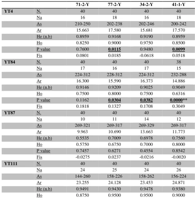
Deviations from HWE were initially detected at loci YT4, YT84, YT111, YT12 and YT29, but after Bonferroni correction only loci YT12 (in all samples) and YT84 (only in sample 41-1-Y) were still significant. This significance is likely, related to high positive FIS values, suggesting deficiency of heterozygous genotypes as already highlighted with the MICROCHECKER assessment.
Tab. 5_Genetic diversity estimates: Single-locus and mean values are given. N= number of samples analysed; Na= number of alleles; As= allelic size range; Ar= allelic richness; He (n.b)= expected non biased heterozygosity; Ho= observed heterozygosity; Fis= inbreeding coefficient. Bold and underlined values indicated a significant HW disequilibrium (P<0.05); Significance after sequential Bonferroni’s correction is described as follows: *P < 0.05; **P < 0.01.
71-2-Y 77-2-Y 34-2-Y 41-1-Y
YT4 N. 40 40 40 40 Na 16 18 16 18 As 210-250 202-238 202-246 200-242 Ar 15.663 17.580 15.681 17.570 He (n.b) 0.8959 0.9168 0.9190 0.8959 Ho 0.8250 0.9000 0.9750 0.8500 P value 0.7600 0.0115 0.9480 0.0099 Fis 0.0801 0.0185 -0.0618 0.0518 YT84 N. 40 40 40 38 Na 17 16 17 15 As 224-312 228-312 224-312 232-288 Ar 16.300 15.590 16.373 14.886 He (n.b) 0.9146 0.9209 0.9025 0.9049 Ho 0.7500 0.8000 0.7500 0.6316 P value 0.1162 0.0304 0.0382 0.0000** Fis 0.1818 0.1327 0.1708 0.3049 YT87 N. 40 40 40 40 Na 10 11 14 12 As 269-321 269-317 269-329 269-317 Ar 9.963 10.690 13.663 11.773 He (n.b) 0.5535 0.7009 0.6978 0.7560 Ho 0.5750 0.6750 0.7000 0.8000 P value 0.7457 0.6271 0.4554 0.8542 Fis -0.0275 0.0237 -0.0216 -0.0020 YT111 N. 40 40 40 40 Na 24 25 24 26 As 144-260 158-226 158-262 156-224 Ar 23.255 24.128 23.453 24.871 He (n.b) 0.9491 0.9430 0.9478 0.9380 Ho 0.8750 0.9500 0.9500 0.9000
30 P value 0.3126 0.8055 0.7636 0.0427 Fis 0.0789 -0.0075 -0.0024 0.0410 YT12 N. 39 40 40 40 Na 21 19 22 19 As 313-375 313-371 315-377 317-375 Ar 20.359 18.437 21.553 18.446 He (n.b) 0.9048 0.9022 0.9389 0.8959 Ho 0.3590 0.6500 0.6500 0.4750 P value 0.0000** 0.0000** 0.0000** 0.0000** Fis 0.6064 0.2821 0.3104 0.4730 YT29 N. 40 40 40 36 Na 17 19 17 21 As 171-215 165-223 177-219 161-213 Ar 16.871 18.289 16.581 21.000 He (n.b) 0.9307 0.9222 0.9038 0.9045 Ho 0.8000 0.9500 0.9000 0.7778 P value 0.0051 0.9389 0.2822 0.0144 Fis 0.1420 -0.0306 0.0043 0.1419 YT92 N. 40 40 40 36 Na 13 11 8 12 As 204-232 214-238 214-234 206-238 Ar 12.282 10.582 7.890 11.300 He (n.b) 0.7323 0.7263 0.7633 0.7062 Ho 0.7750 0.6750 0.7250 0.9000 P value 0.3286 0.3279 0.5826 0.5497 Fis -0.0591 0.0714 0.0508 -0.1323 YT121 N. 40 40 40 36 Na 23 22 25 24 As 148-214 154-222 154-210 154-216 Ar 22.436 21.271 24.460 23.318 He (n.b) 0.9399 0.9370 0.9604 0.9364 Ho 0.9250 0.9500 0.9250 0.8500 P value 0.1271 0.2114 0.2311 0.1594 Fis 0.0160 -0.0140 0.0374 0.0933 MEAN He (n.b) 0.8526 0.8712 0.8792 0.8785 Ho 0.7355 0.8187 0.8219 0.7730 P value 0.2139 0.3691 0.4126 0.2038 Fis 0.1258 0.0613 0.0633 0.1143
Although these loci (YT12 and YT84) do not respect the HW equilibrium and possible null alleles may be present, the Jackknife test shows that they do not give different signals respect to the other loci for F statistics values, demonstrating that all loci analysed can be used for this study (Tab. 6).
31
Tab. 6_Jackknife statistic analysis used for variance and bias estimation: FIS (0.01769 - 0.20125); FIT (0.01891 - 0.20462); FST (-0.00025 - 0.00431).
Jackknife FIS FIT FST
YT4 0.10708 0.10875 0.00188 YT84 0.08089 0.08319 0.00250 YT87 0.10796 0.10911 0.00129 YT111 0.10668 0.10835 0.00187 YT12 0.04760 0.04901 0.00149 YT29 0.10101 0.10254 0.00170 YT92 0.10992 0.11191 0.00224 YT121 0.10579 0.10821 0.00271 Mean 0.09662 0.9838 0.00194
Data showed the presence of problematic loci that do not respect the HW equilibrium. These loci may affect final results, for this reason we performed several tests to check out how they would influence the genetic differentiation analyses.
Three tests were conducted: the first one excluding locus YT12 from the dataset, the second excluding locus YT84 and the last with the exclusion of both these two loci. In general results obtained showed very similar Fst patterns and values (Appendix 2). For this reason, we will show here only the analysis carried out with all available loci.
Pairwise Fst analysis did not reveal any significant divergence among population samples (Tab. 7), except one comparison, retaining significance also after Bonferroni correction, between samples 71-2-Y (WCPO) and 41-1-Y (WCAO) (Fst = 0.00927, P= 0.00218).
Tab. 7_Pairwise Fst values (below the diagonal) and associated significance pValue (above the diagonal). Significance after sequential Bonferroni’s correction is described as follows: (*P < 0.05; **P < 0.01).
Fst 71-2-Y 77-2-Y 34-2-Y 41-1-Y
71-2-Y - 0.40600 0.07207 0.00218*
77-2-Y 0.00162 - 0.60469 0.36957
34-2-Y 0.00454 0.00011 - 0.78913
32
Principal coordinates analysis (PCoA) based on the pairwise Fst matrix were performed to assess differentiation among samples (Fig. 14). The scatter plot obtained showed on the first axis differentiations between Atlantic Ocean (41-1-Y and 34-2-Y) and West Pacific Ocean (71-2-Y) samples, while the East Pacific Ocean one (77-2-Y) is differentiated from the others on the second axis. However, first axis and second axis do not explain most of the variation, representing respectively 51.23 % and 25.23 %.
Fig. 14_Principal Coordinates Analysis (PCoA) of YFT population samples. Scatter plots built on the first two principal coordinates (coordinate 1, x axis; coordinate 2, y axis) based on the pairwise Fst values.
AMOVA analyses were carried out using different samples grouping (Tab. 8): 1) grouping samples per Ocean (Pacific Ocean vs Atlantic Ocean) (AMOVA 1) and 2) following PCoA result (Atlantic Ocean and West Pacific Ocean vs East Pacific Ocean) (AMOVA 2).
Results showed highest percentage of molecular variation within samples (AMOVA 1= 99.61% and AMOVA 2= 99.46%) and low values among group and among samples within group. The subdivision of samples in two groups (Atlantic Ocean and Pacific Ocean) was not statistically significant (AMOVA 1: Fct = 0.0034; P = 0.11144) as well the subdivision based on PCoA results (Atlantic Ocean and West Pacific Ocean vs East Pacific Ocean) (AMOVA 2: Fct = 0.031; P = 0.12512). 71-2-Y 77-2-Y 34-2-Y 41-1-Y Co o rd . 2 - 25, 23 Coord. 1 - 53,24 PCoA
33
Tab. 8_AMOVA statistical analysis.
AMOVA 1
PACIFIC OCEAN and ATLANTIC OCEAN
Variation (%) F - Statistic pValue Among groups 0.34 0.0034 0.11144
Among samples within groups 0.05 0.0005 0.67155
Within samples 99.61 0.0034 0.31672
Yellowfin tuna population structure was further investigated with STRUCTURE individual-based analyses Bayesian clustering. Data output obtained were displayed with STRUCTURE HARVESTER (Web version 0.6.94 July 2014) (Tab. 9).
AMOVA 2
ATLANTIC / W. PACIFIC and E. PACIFIC
Variation (%) F - Statistic pValue Among groups -0.31 0.031 0.12512
Among samples within groups 0.32 0.00315 0.78006
34
Tab. 9_ STRUCTURE HARVESTER summary
K Reps Mean LnP(K) Stdev LnP(K) Ln'(K) |Ln''(K)| ∆K
1 5 -6702,02 0,55 - - - 2 5 -6834,54 10,97 -132,52 46,54 4,24 3 5 -7013,60 82,27 -179,06 151,98 1,85 4 5 -7344,64 381,93 -331,04 197,08 0,52 5 5 -7478,60 277,34 -133,96 138,16 0,50 6 5 -7474,40 162,63 4,20 396,22 2,44 7 5 -7866,42 325,83 -392,02 11,12 0,03 8 5 -8269,56 297,80 -403,74 712,88 2,39 9 5 -7959,82 119,09 309,74 656,90 5,52 10 5 -8306,98 238,72 -347,16 - -
The most likely cluster number (K) identified by the program was inferred with Pritchard method (Pritchard et al., 2000). This theory analyse LnP(K) (the logarithm of the probability of the data given K) trends identifying possible K value as the nearest value to “plateau” (Fig. 14). In fact, STRUCTURE usually run for several values of K, lnP(K) is computed for each of them and plotted against K. Thus, if several values of K give similar estimates of LnP(K), the smallest seems to be the most real. No “plateau” was detected in our analysis, suggesting the lack of samples differentiation (Fig. 15).
35
According with Evanno et al., (2005) the likely number of K populations can also be inferred by the correlation between the second rates of change of LnP”(K) with respect to K (∆K). This method seems to show a clear peak at the true value of K.
In fact authors found the modal value of the distribution of ∆K that represent the real K, and used the height of this value as an indicator of the strength of the signal detected by structure.
In Fig. 16 is showed the ∆K value respect to K obtained for this study.
Results are discordant to the previous LnP(K) assessment, in fact the function ∆K presents the maximum values at K=2, K=6 and K=9.
Considering both methods and the different K values obtained, we can presume that K=6 and K=9 are not realistic to correctly represents yellowfin tuna population.
Fig. 16_Evanno’s absolut ∆K graph.
For K=2 barplot obtained showed clearly the absence of any structuring between Atlantic and Pacific YFT samples (Fig. 17). In fact, all samples showed a genetic composition whose percentage values of individual membership revealed a total admixture between them.
36
Fig. 17_ Estimated membership fraction of individuals from each sampling area : (1)= 71-2-Y; (2)= 77-2-Y; (3)=34-2-Y; (4)=41-1-Y
71-2-Y 77-2-Y 34-2-Y 41-1-Y
37
6. Discussions and conclusions
6.1 Species identification for YFT juveniles
Species identification of tuna juveniles is essential to increase the information on the real by-catch data, contributing decisively to more tangible and functional management plans. Unfortunately, it is quite difficult when morphological features are ambiguous or missing, such as with frozen specimens.
The immature tuna by-catch is abundantly underestimated and unreported in the fishermen's logbook worldwide (Amandè et al., 2010). In fact fishermen usually do not report the real amount of little tunas by-catch because of their discard at the sea or their parallel importance in the local markets, as for instance the local market of Abidjan (Central-West Africa) (Romagny et al., 2000).
However, since 2001 the European Union (EU) has developed a mandatory sampling program for the collection of data in the fisheries sector under the EU Data Collection Regulation (DCR) directive in support of its Common Fishery Policy, with the specific objective to evaluate the real amount of by-catch and discards in these fisheries (Amandè et al., 2010).
By contrast, in population structure studies, the collection of juveniles (i.e. post-larval and early-stage juvenile), according to their limited capacity to swim than the older ones, would increase the likelihood to work with individuals caught close to their nursery areas, detecting the genetic composition of the spawning populations (Carlsson et al., 2007). However, post-larval and early-stage juveniles of many tuna and tuna-like species are morphologically similar between them, especially if they belong to the same genus (Robertson et al., 2007) and their identification requires high-quality taxonomic skills. Furthermore, species misidentification at early juvenile’s stage could be caused by geographical variation in their morphological features (Chow and Inoue 1993). Also, the use of morphological characters (such as body shape, pigments, characteristics of the fins, etc.) is deceptive when for instance individuals are frozen or exposed to other processes (e.g. canning, filleting) which make the species identification almost impossible.
These problems could affect their real mortality information and make stock assessment more difficult.
38
The molecular approach is one of the most powerful and concrete among the different methodologies developed to overcome species misidentification problems (Teletchea et al., 2009).
Many different DNA sequences have been used for helping with tuna and tuna-like species identification. Some tuna and tuna-like species are very close genetically and hybridization among species would create taxonomic uncertainty (Ward et al., 2005) with mitochondrial introgression patterns that have been described for some of them (Alvarado Bremer et al., 2005).
Among the different species of the genus Thunnus, species identification is particularly challenging between BET and YFT that are usually caught together with FAD-sets, due to the genetic nearby . Thus, a specific gene marker has to be selected appropriately and detailed knowledge of the DNA sequences from target species are required before setting-up the methodology and validate the final assignation. Several attempts have been done, employing different markers, to discriminate between YFT and BET, and their results were not always satisfying. In this study the use of mtDNA fragment ATCO to identify YFT specimens and to avoid any possible misidentification with BET juveniles, was a fitting choice. Our results showed the absence of variable sites between our YFT sequences and those taken from Genbank (www.ncbi.nlm.nih.gov/genbank/) confirming their high reliability. In the alignment produced 109 variable sites (V) and 15 informative sites (Pi) were detected. The Neighbour-Joining tree obtained, using Tamura-Nei distance method separated the 66 samples collected in the western part of the Pacific ocean and identified as YFT by our collaborator from 5 BET that were personally sampled in the Gulf of Guinea (with bootstrap values of 95% and 99% respectively). Our results confirmed the results of Chow and Inoue (1993), underlying the suitability of ATCO as molecular marker to discriminate between the two widely harvested species. However further tests are requested with a higher number of specimens, sampled in other fishing areas, to really assess its reliability for management purposes.
Nevertheless, previous studies carried out with RFLP analysis do not showed any concreteness in discriminating between these species. Instead the triplex-PCR approach devised by Michelini et al., (2007) through ctyb analysis, seems to be a very practical reliable and economical technique. In addition the results are simply obtained during the course of a PCR reaction, without the need of expensive sequencing.