3D reconstruction from 2D sections via genetic algorithms : an application to metallic fuel

(1)

POLITECNICO DI MILANO

Dipartimento di Energia

Divisione di Ingegneria Nucleare

3D RECONSTRUCTION FROM 2D SECTIONS

VIA GENETIC ALGORITHMS:

AN APPLICATION TO METALLIC FUEL

Relatore: Davide Pizzocri

Correlatori: Fabiola Cappia

Tommaso Barani

Tesi di Laurea Magistrale di:

Riccardo Genoni, 895376

Anno accademico 2018/2019

(2)

(3)

Acknowledgements

I

Acknowledgements

This work is the result of the collaboration between the Nuclear Reactors Group of the Department of Energy of Politecnico di Milano and the Post-Irradiation Examination (PIE) Division of the Metallic Fuel Complex (MFC) of Idaho National Laboratory (INL). It was partly funded by:

• The U.S. Department of Energy – Nuclear Energy Office (DOE-NE). • Nuclear Science User Facilities (NSUF) Project 428 17-091.

• The Advanced Fuel Campaign (AFC) of the Nuclear Technology Research and Development Program.

My most sincere thanks go my supervisor Dr. Davide Pizzocri for the support, guidance and oversight provided throughout the whole period of work.

I also want to thank my assistant supervisor Tommaso Barani for the support ad advice provided during my stay in Politecnico di Milano.

My deepest gratitude goes to my mentor at INL, Dr. Fabiola Cappia for the dedication, commitment, and counsel throughout the months spent in the U.S. Her diligence, hard work, and organizational ability were fundamental to the good outcome of this endeavor. I wish to express my indebtment to Prof. Lelio Luzzi, who has always shown the keen-est interkeen-est in the good outcome of this endeavor, for the great opportunity to work in this collaboration between Politecnico di Milano and INL that I was offered.

I also thank Federico Antonello for the fruitful discussion, and constructive advice on the development of the genetic algorithm.

I want to thank my colleagues, whom I have rejoiced and suffered with throughout my course of studies for the Master of Science in Nuclear Engineering.

I give my thanks my family, for the upbringing and example I was given as a boy. There is no growth without toil, no retribution without sweat, and no achievement without

(4)

Acknowledgements

II

discipline. Hard lessons I have striven to learn, and which I could have never appreciated without the raising I was given. Without these lessons, these five years may not have been five, and tenacity might have failed me the many times I most needed it.

Last but not least, I want to acknowledge Silvia, the person that has become truly im-portant for me in these days. Personal order and private peace are truly fundamental for the accomplishment of any endeavor. Her presence has provided both, and whatever the outcome be, I shall always be grateful to her.

(5)

Acknowledgements

III

A Vittorio Miele (18/07/1934 — 26/11/2014)

(6)

Abstract

IV

Abstract

Porosity is one of the main properties that affects irradiation performance of nuclear fuel. Its measurement and study his crucial for the characterization of innovative fuel concepts, such as metallic fuels, the performance of which is still under scrutiny.

The development of porosity impacts important phenomena such as phase formation, components migration, fission gas release, gas driven swelling, and thermal conductivity. The property of percolation threshold specifically—i.e., the limit porosity at which the porous material percolates—is extremely significant, since it governs the transport of fis-sion products within the fuel itself. Percolation is a property that can be obtained only directly from 3D information on the porous material. This kind of information is however not always available, as direct methods to gain it—such as micro computed tomography (Micro-CT) and focused ion beam sectioning and scanning (FIB)—have serious limita-tions with dense irradiated materials and large volumes. Therefore, a simpler way to pro-ceed is to adopt a reconstruction procedure that from images of 2D sections of experi-mental samples can extract statistical information on the 3D microstructure. From this, useful information can be gained, and percolation threshold can be computed.

There are several reconstruction procedures that have been introduced in other works. However, the complexity of the microstructure of metallic fuel makes necessary to intro-duce a new approach. Genetic Algorithms have several good properties that make them attractive in solving complex reconstruction problems. In this work a reconstruction pro-cedure based on a Genetic Algorithm was proposed. This was verified against known 3D microstructures, then apply it to experimental samples taken from DOE-1 metallic fuel from FUTURIX-FTA irradiation campaign.

(7)

Sintesi

V

Sintesi

La porosità del combustibile nucleare è una delle principali proprietà che ne influenzano il comportamento durante l’irraggiamento in reattore. Di conseguenza, la caratterizzazione della porosità e della sua evoluzione è cruciale per lo sviluppo di combustibili innovativi, come il combustibile metallico.

Diversi fenomeni fisici peculiari del combustibile, quali la formazione di fasi, il rila-scio dei gas, il rigonfiamento da gas e la conducibilità termica sono influenzati dalla pre-senza e dalle caratteristiche della porosità. In particolare, la soglia di percolazione—la porosità limite alla quale un materiale poroso percola—è estremamente significativa, dal momento che governa il trasporto di prodotti di fissione nel combustibile. La percolazione è una proprietà intrinsecamente 3D e può essere ricavata solo tramite una conoscenza della struttura tridimensionale della proprietà. Questa conoscenza non è sempre disponibile spe-rimentalmente, essendo i metodi diretti per ottenerla—come micro-tomografia a raggi X (Micro-CT) e il sezionamento e ricostruzione con fascio di ioni focalizzati (FIB)— inap-plicabili a materiali densi (quali il combustibile) e grandi volumi (necessari per la natura statistica della struttura).

Vista la difficoltà di caratterizzare sperimentalmente la porosità in 3D, l’approccio ca-nonico è quello di impiegare metodi di ricostruzione che, partendo da immagini di sezioni sperimentali 2D, estraggano informazioni statistiche sulla microstruttura 3D. Da questa, si possono ottenere informazioni per calcolare, ad esempio, la succitata soglia di percola-zione.

Diversi metodi di ricostruzione sono disponibili in letteratura, ciascuno basato su pe-culiari ipotesi stereologiche e processi di ottimizzazione. Tuttavia, la complessità della

(8)

Sintesi

VI

microstruttura della microstruttura 3D del combustibile nucleare (e metallico in partico-lare) rende necessario il rilassamento di alcune ipotesi di ricostruzione e la scelta di op-portuni metodi di ottimizzazione. In questo lavoro di tesi si propone un nuovo metodo di ricostruzione basato su un algoritmo genetico e sulla definizione di una funzione obiettivo che sia slegata da precise ipotesi sulla struttura 3D da ricostruire. Il nuovo metodo è stato verificato su microstrutture 3D virtuali di riferimento, e quindi applicato alla ricostruzione di campioni di combustibile metallico DOE-1 della campagna di irraggiamento FUTU-RIX-FTA.

(9)

Estratto in Italiano

VII

Estratto in Italiano

Introduzione

La conoscenza delle proprietà della microstruttura 3D di un materiale è spesso fondamen-tale per poterne ricavare le proprietà termofisiche e studiarne il comportamento integrale. Questo è tanto più importante nello studio dei materiali nucleari, permettendo di cono-scerne accuratamente proprietà con effetti determinanti dal punto di vista della sicurezza, come ad esempio la conducibilità termica e la soglia di percolazione. In questo lavoro ci si concentra su quest’ultima proprietà, la quale ha un ruolo estremamente importante nel determinare il rigonfiamento dovuto ai gas di fissione (gaseous swelling) in combustibili metallici. La soglia di percolazione viene definita come la soglia di porosità di un mate-riale affinché questo possa percolare in ciascuna delle tre direzioni. È influenzata da vari fattori, come la struttura dei pori, la loro distribuzione e la loro dimensione, tutte proprietà che possono essere direttamente ricavate solo con una conoscenza della microstruttura porosa 3D del materiale di interesse.

Non sempre è possibile ottenere direttamente questo genere di informazioni, specie se queste sono necessarie su larghi volumi di materiale irraggiato. Metodi esemplari utilizzati nello studio delle microstrutture 3D sono la micro-tomografia a raggi X (Micro-CT) e il sezionamento e ricostruzione con fascio di ioni focalizzati (FIB). Il primo metodo sfrutta fasci di raggi X per studiare le microstrutture, ed è limitato dalla penetrazione degli stessi nel materiale che si intende studiare. Di conseguenza si rivela poco pratico in materiali ad alta densità. Il secondo metodo FIB invece è un metodo distruttivo, il campione viene eroso dai fasci di ioni e, visti gli alti costi, può essere utilizzato su volumi molto ridotti. Un’altra importante limitazione di entrambi questi metodi—specificamente nel campo nu-cleare—è che non possono essere applicati in cella calda a materiale irraggiato per un gran numero di campioni. Per queste ragioni, si è indagato molto sulla possibilità di

(10)

VIII

applicazione di metodi di ricostruzione per microstrutture 3D partendo da informazioni ottenibili dalle sezioni 2D tagliate da campioni sperimentali. L’idea è quindi di applicare un metodo non distruttivo e semplice che permetta di ottenere un’informazione indiretta sulla microstruttura 3D e che non sia sottoposto alle limitazioni dei metodi già citati.

Le procedure di ricostruzione si propongono di risolvere un problema inverso partendo da strutture 2D ricostruendo strutture 3D, quindi ricavando da un grado d’informazione minore uno maggiore. La microstruttura ricavata può essere quindi una realizzazione sta-tisticamente simile al riferimento che si intende ricostruire. Un modo di procedere è trat-tare il problema come un problema di ottimizzazione, aprendo nuove opportunità all’ap-plicazione di metodi euristici come gli algoritmi genetici. La grande problematica è tutta-via la capacità di simili metodi di poter essere utilizzati nella ricostruzione di microstrut-ture porose complesse come nel caso del combustibile metallico.

L’obiettivo di questo lavoro è dunque lo sviluppo di una procedura basata su un algo-ritmo genetico per la ricostruzione statistica di microstrutture porose 3D partendo dall’im-magine 2D di una sezione tagliata dal campione di riferimento. Questa procedura verrà validata su delle microstrutture artificiali note di complessità differente. In seguito, una volta verificata la capacità di riprodurre microstrutture complesse, questa sarà applicata alla ricostruzione, partendo da dati sperimentali prelevati da combustibile metallico DOE-1 proveniente dalla campagna di irraggiamento FUTURIX-FTA del Dipartimento dell’Energia USA.

L’informazione ricavata produrrà una serie di microstrutture 3D che sono le migliori candidate a essere il riferimento sperimentale. Queste verranno utilizzate per calcolare la frazione di volume percolante sul volume totale, parametro che può essere utilizzato per inferire la frazione di percolazione in strutture a bassa porosità.

(11)

IX

Parte Prima

Sviluppo della procedura di ricostruzione

Nella prima parte di questo lavoro si tratta dello sviluppo e della validazione della proce-dura di ricostruzione. Il problema della ricostruzione è un problema inverso. L’obiettivo è inferire informazione di grado di complessità più alto da informazioni di grado di com-plessità più basso. È necessario in primo luogo adottare un modello matematico del si-stema che possa essere definito in termini di funzioni statistiche [1].

Il random heterogeneous material (RHM) è il modello adottato per la procedura di ricostruzione di interesse. L’RHM è un qualsiasi materiale solido caratterizzato da due o più fasi materiali le quali soddisfano l’ipotesi di isotropia. In aggiunta, il sistema è tale per cui lunghezze caratteristiche delle fasi materiali sono maggiori delle lunghezze molecolari e minori delle lunghezze macroscopiche dei campioni [2].

Si consideri in questo lavoro un materiale bifase costituito da una fase materiale e una fase porosa. Quest’ultima costituisce la fase di interesse e viene descritta in termini stati-stici per mezzo delle correlazioni a n-punti. Nello specifico in questo lavoro se ne use-ranno tre, le quali portano informazione sufficiente per la ricostruzione:

• Correlazione a un punto, la probabilità che campionato un punto all’interno del volume questo cada in fase porosa;

• Correlazione a due punti, la probabilità che campionati due punti all’interno del volume entrambi cadano in fase porosa (la correlazione va calcolata in funzione della distanza fra i due punti);

• Funzione di percorso lineare, la probabilità che campionato un segmento all’in-terno del volume, questo cada interamente in fase porosa (la correlazione va cal-colata in funzione della lunghezza del segmento).

Queste correlazioni presentano nel caso dell’RHM delle favorevoli proprietà per la procedura di ricostruzione. Infatti, l’isotropia garantisce che queste siano invarianti alla direzione a cui si calcolano, e che al limite di volume infinito le correlazioni 3D e 2D si scostino fra di loro solo per un errore infinitesimale [3].

(12)

X

Di conseguenza le correlazioni diventano le grandezze di riferimento per la ricostru-zione e per verificare qualora la procedura abbia avuto buon fine. Un’altra informaricostru-zione utile della microstruttura 3D non ricavabili direttamente dalle informazioni della sezione 2D è la distribuzione della dimensione dei pori (pore-size distribution, PSD). Questa rap-presenta una distribuzione statistica dei pori rispetto ai raggi equivalenti dei pori. Può es-sere ricavata sia in 2D che in 3D, ma non esiste fra le due una relazione matematica forte come fra le correlazioni 2D e 3D [3].

Tradizionalmente, la ricostruzione di un mezzo poroso è il soggetto della stereologia, laddove trova applicazione il metodo Schwartz-Saltykov, già utilizzato per la ricostru-zione della porosità in combustibili ossidi per Reattori ad acqua [4]. Questo metodo si basa tuttavia su ipotesi molto forti e ha di conseguenza applicazioni limitate per quanto riguarda il combustibile metallico. Da qui deriva la necessità di sviluppare procedure di ricostruzione basate su problemi di ottimizzazione che sfruttino l’informazione morfolo-gica (statistica, funzioni di correlazione…) del 2D per riprodurre il 3D originario [5].

Sono state proposte diverse tecniche in altri lavori [3], [5]–[7]. La complessità del pro-blema ha reso necessaria l’adozione di tecniche euristiche che permettessero di identifi-care più facilmente la soluzione del problema di ricostruzione (l’ottimo globale del pro-blema di ottimizzazione).

La scelta è caduta sull’algoritmo genetico. L’algoritmo genetico è un metodo euristico facente parte della famiglia degli algoritmi evolutivi [8]. Esso è un metodo di ricerca glo-bale [5], che presenta ottime proprietà di esplorazione e sfruttamento [9], e produce alla fine non una singola soluzione, ma una famiglia di migliori soluzioni. Essendo un metodo euristico, si presenta come una procedura quasi-casuale [10]; l’ottimizzazione procede ite-rativamente e indipendentemente dalle caratteristiche del problema (e.g. il gradiente). In quanto metodo evolutivo, l’algoritmo genetico si divide in due fasi principali:

• Inizializzazione, in cui si inizializza una serie (popolazione) iniziale di soluzioni del problema di ottimizzazione (individui). Questi sono campionati casualmente all’interno dello spazio di ricerca iniziale.

• Generazione, è la fase iterativa in cui la popolazione precedente viene confrontata con il riferimento tramite una funzione di fitness e viene classificata. L’informa-zione degli individui migliori (padri) viene poi utilizzata per produrre la

(13)

XI

popolazione successiva (figli). Il procedimento è ripetuto finché non si ottiene come risultato la convergenza.

La nuova popolazione prodotta a ogni generazione avrà qualità migliori della genera-zione precedente [11]. L’obiettivo della procedura di ricostrugenera-zione è produrre delle micro-strutture 3D (le soluzioni del problema) che verranno poi tagliate per estrarne la sezione 2D. le proprietà della sezione vengono utilizzate per definire il problema e la funzione di fitness. L’obiettivo è ottenere alla fine delle microstrutture 3D che riproducano sezioni 2D che siano statisticamente identiche alla sezione 2D di riferimento. Questa popolazione di soluzioni finali sarà la serie di migliori candidati a ricostruire la microstruttura di riferi-mento (a priori ignota). Il confronto nella fase di ricostruzione viene fatto mediante le correlazioni, che costituiscono in diversi altri lavori la base dei procedimenti di ricostru-zione [3], [5]–[7].

Tuttavia, visto il legame matematicamente forte fra le correlazioni in 2D e 3D, è stata preferita in questo lavoro una funzione di fitness che fosse meno vincolante e lasciasse più gradi di libertà alla ricostruzione. Di conseguenza si basa la ricostruzione sui parametri della PSD (raggio equivalente medio e deviazione standard) e sul numero di pori della sezione 2D. La procedura così prodotta deve essere validata prima di essere applicata ai dati sperimentali.

La validazione viene fatta su microstrutture 3D di riferimento artificiali, di cui si co-nosce a priori tutte le caratteristiche. In particolare il lavoro si concentra su due famiglie: la più semplice, in cui i pori sono modellizzati come sfere sovrapponibili della stessa di-mensione, e una più complessa, sebbene più fisica rispetto ai processi considerati nella seconda parte di questo lavoro [12], che vede sfere la cui dimensione è distribuita come una log-normale.

Modello a dimensione singola

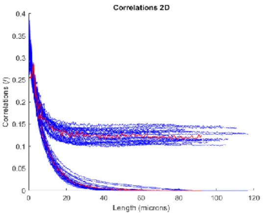
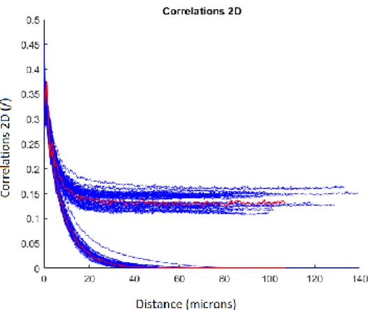
Le correlazioni sulle sezioni 2D degli elementi appartenenti al fronte di Pareto [13] corri-spondono alle correlazioni 2D del riferimento (Figure 0.1) e lo stesso si può dire delle correlazioni 3D (Figure 0.2). Stando alle immagini delle sezioni non c’è visibilmente nes-suna differenza statistica fra le due, come visibile in Figure 0.3 e in Figure 0.4. Questo si riflette nelle correlazioni.

(14)

XII Figure 0.1. Correlazioni 2D di riferimento (rosso) vs.

ricostruite (blu), distanza in µm (orizzontale) vs. cor-relazione a due-punti e funzione a percorso lineare.

Figure 0.2. Correlazioni 3D di riferimento (rosso) vs. rico-struite (blu), distanza in µm (orizzontale) vs. correlazione a due-punti e funzione a percorso lineare.

Figure 0.3. Sezione 2D di riferimento. Figure 0.4. Sezione 2D ricostruita.

Modello log-normale

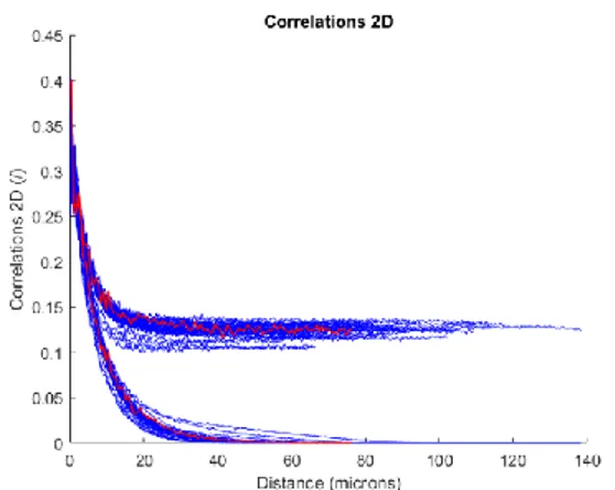
Le correlazioni sul 2D corrispondono alle correlazioni 2D del riferimento (Figure 0.5) e lo stesso si può dire delle correlazioni 3D (Figure 0.6). Allo stesso modo osservando le im-magini delle sezioni non si notano alcune differenze statistiche fra le due, come è evidente dalla Figure 0.7 e Figure 0.8.

(15)

XIII

Figure 0.5. Correlazioni 2D di riferimento (rosso) vs. ricostruite (blu), distanza in µm (orizzontale) vs. corre-lazione a due-punti e funzione a percorso lineare.

Figure 0.6. Correlazioni 3D di riferimento (rosso) vs. ricostruite (blu), distanza in µm (orizzontale) vs. corre-lazione a due-punti e funzione a percorso lineare.

Figure 0.7. Sezione 2D di riferimento. Figure 0.8. Sezione 2D ricostruita.

La procedura di ricostruzione si rivela dunque efficacie nella ricostruzione di microstrut-ture anche complesse come quella descritta dalla log-normale. Si è ottenuta una buona convergenza in entrambi i casi al minimo globale, verificata con il confronto fra le corre-lazioni 3D del riferimento e delle microstrutture ricostruite. Si osservi anche la somi-glianza fra le correlazioni 2D e 3D, derivante dalle proprietà dell’RHM [2].

Il metodo genera una serie consistente di microstrutture con caratteristiche morfologi-che molto simili, ognuna delle quali rappresenta una diversa realizzazione della fase po-rosa. Quello che si è ottenuto è un intervallo di confidenza di strutture porose 3D che possono aver prodotto la sezione 2D di riferimento. Questo è un particolare fondamentale che ci permette di ottenere degli intervalli di confidenza sulle proprietà 3D del riferimento.

(16)

XIV

Calcolo della Frazione di Percolazione

L’informazione raccolta può essere sfruttata per calcolare la frazione di percolazione di microstrutture 3D, un parametro utile per il calcolo della frazione di percolazione [14]. Gli algoritmi di percolazione lavorano però su matrici discrete. È importante indagare quali siano gli effetti della discretizzazione in termini di risoluzione e di connettività fra i voxel della matrice 3D sul calcolo della frazione di percolazione. Come risoluzione si è adottata la risoluzione tipica dell’image analysis da immagini sperimentali prese con microscopia ottica (OM), che è circa di 5 lati di pixel per micron [15].

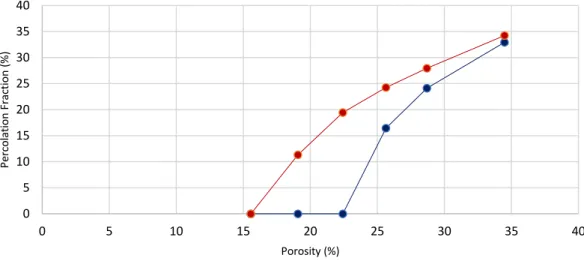
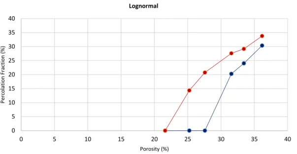
Per quanto riguarda la connettività fra i voxel, si è fornito un limite superiore e inferiore per il calcolo della frazione percolante in base al numero di possibili percorsi introdotti dalle diverse connettività (maggiore la connettività, maggiore il numero di percorsi). In questo modo si forniscono dei limiti inferiori e superiori che rappresentano fisicamente il minimo e il massimo volume percolante descrivibile. Si forniscono i risultati sia per il modello a dimensione singola, sia per il modello log-normale.

Figure 0.9. Curve di frazione percolante per dimensione singola, connettività 26 (rosso) vs. connettività 6 (blu).

0 5 10 15 20 25 30 35 40 0 5 10 15 20 25 30 35 40 P er co lat io n Fr ac ti o n ( %) Porosity (%) Single Size

(17)

XV

Figure 0.10. Curve di frazione percolante per distribuzione log-normale, connettività 26 (rosso) vs. connettività 6 (blu). 0 5 10 15 20 25 30 35 40 0 5 10 15 20 25 30 35 40 P er co lat io n Fr ac ti o n ( %) Porosity (%) Lognormal

(18)

XVI

Parte Seconda

Applicazione ai dati sperimentali

Una volta che si è verificata la capacità della procedura di ricostruzione di riprodurre fe-delmente le microstrutture 3D dei materiali di riferimento partendo da sezioni di questi, è possibile applicarla a immagini sperimentali le cui corrispondenti informazioni 3D sono a

priori ignote. A questo punto, la procedura di ricostruzione e il calcolo di percolazione

vengono applicati a immagini provenienti da campioni di combustibile metallico. Il com-bustibile in considerazione è il DOE-1 irraggiato nella campagna sperimentale FUTURIX-FTA nel reattore Phénix in Francia, frutto dalla collaborazione fra lo U.S. Department of Energy (U.S. DOE) e fra il Commissariat à l’Énergie Atomique et aux Energies Alterna-tives (CEA).

Il combustibile metallico presenta diversi vantaggi rispetto al combustibile ossido: ha caratteristiche di sicurezza intrinseca, può essere utilizzato per la trasmutazione degli at-tinidi minori e del plutonio estratti tramite riprocessamento da combustibile già utilizzato in reattori ad acqua, ed è compatibile con i processi di riciclo pirometallurgico, il che lo rende apprezzabile dal punto di vista della prevenzione della proliferazione nucleare [16]. Il DOE-1 appartiene alla famiglia dei combustibili ternari, costituiti da una lega metallica di U-Pu-Zr. Nello specifico, si tratta di un combustibile ad alta concentrazione di Zr, la cui composizione nominale è U-29Pu-4Am-2Np-30Zr [17].

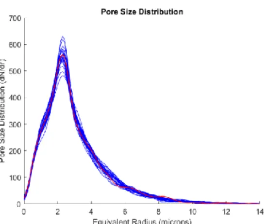
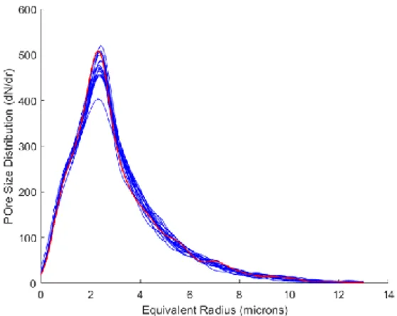
Durante l’irraggiamento, il combustibile DOE-1 ha sviluppato una porosità intercon-nessa caratterizzata da pori di forme complesse che possono essere modellizzati come sfere sovrapponibili isotropicamente distribuite nel volume del solido. Il materiale può essere efficacemente modellizzato come un RHM e quindi è possibile applicare la proce-dura di ricostruzione sviluppata in questo lavoro. Questa è stata impiegata con successo dal momento che le sezioni 2D delle microstrutture 3D ricostruite risultavano essere stati-sticamente identiche alle sezioni 2D di riferimento. Si mostra nelle figure successive il risultato di una ricostruzione da un’immagine del DOE-1, evidenziando la convergenza sulla distribuzione della dimensione dei pori 2D (Figure 0.11) e sulle correlazioni 2D

(19)

XVII

(Figure 0.12). Sono mostrate anche la sezione di riferimento (Figure 0.13) confrontata a una delle sezioni ricostruite (Figure 0.14).

Figure 0.11. Distribuzione della dimensione dei pori 2D di riferimento (rosso) vs. ricostruita (blu), dimensione dei pori in µm (orizzontale) vs. numero di pori differen-ziale (verticale).

Figure 0.12. Correlazioni 3D di riferimento (rosso) vs. ricostruite (blu), distanza in µm (orizzontale) vs. corre-lazione a due punti e funzione di percorso lineare (verti-cale).

Figure 0.13. Sezione 2D di Riferimento. Figure 0.14. Sezione 2D ricostruita.

Una volta conclusa la ricostruzione, il calcolo di percolazione è stato applicato, ricavando per ciascuna microstruttura ricostruita la corrispondente frazione di percolazione (i.e. la frazione di volume di pori percolanti su volume totale). È stato in seguito possibile rica-vare un valore di media e di deviazione standard della frazione percolante, producendo un intervallo di confidenza sulla percolazione del mezzo poroso di riferimento.

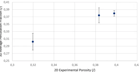
Si mostra in Figure 0.15 i risultati del calcolo della frazione di percolazione in un caso di applicazione a un’immagine del DOE-1. In Figure 0.16 si mostra invece il grafico dei risultati per tre immagini, mettendo in relazione la porosità 2D di queste con la frazione

(20)

XVIII

percolante media calcolata sulle strutture ricostruite con i rispettivi intervalli di confi-denza. L’applicazione della procedura di ricostruzione può essere utilizzata per ottenere maggiori dati con cui costruire una relazione empirica fra la porosità 2D del combustibile metallico e la frazione percolante 3D. Con questa relazione è possibile in seguito estrapo-lare il valore della soglia di percolazione.

Figure 0.15. Porosità vs. frazione di percolazione delle microstrutture 3D ricostruite (blu), e porosità media vs. fra-zione di percolafra-zione media di tutte le realizzazioni (rosso).

Figure 0.16. Porosità Misurata dalle immagini sperimentali 2D vs. la frazione di percolazione media misurata dalle microstrutture 3D ricostruite. 0,355 0,36 0,365 0,37 0,375 0,38 0,385 0,39 0,37 0,375 0,38 0,385 0,39 0,395 0,4 Perc o lat ion Fra ctio n Porosity 0,25 0,27 0,29 0,31 0,33 0,35 0,37 0,39 0,41 0,3 0,32 0,34 0,36 0,38 0,4 0,42 3D Av era ge Perc o lat ion Fra ctio n (/) 2D Experimental Porosity (/)

(21)

XIX

Conclusioni

In questa tesi si propone e verifica una nuova procedura di ricostruzione di una struttura 3D (per semplicità e senza perdita di generalità si considera un mezzo poroso con due fasi) a partire da sue sezioni 2D. La procedura proposta usa un algoritmo genetico che risolve un problema di ottimizzazione multi-obiettivo, minimizzando la differenza fra le proprietà (numero di pori, dimensione media dei pori e varianza della dimensione dei pori) di una sezione 2D di riferimento e le proprietà delle sezioni 2D estratte dalle strutture 3D rico-struite. È importante notare che:

• L’uso di un algoritmo genetico permette di affrontare un problema di ottimizza-zione su base euristica senza la necessità di definire un funzionale nello spazio di ricerca. La soluzione del problema di ottimizzazione non è unica, ma è rappresen-tata da un insieme di strutture 3D “ugualmente ottime” (fronte di Pareto). Proprio questa non-unicità della soluzione permette di associare intervalli di confidenza ai risultati della ricostruzione.

• La procedura proposta permette di inferire proprietà 3D a partire da proprietà mi-surabili sulle sezioni 2D. Infatti, se per alcune proprietà e sotto opportune ipotesi (e.g., porosità in mezzi isotropi) esistono teoremi che dimostrano la corrispon-denza statistica dei valori 2D e 3D, questo non è vero in generale, ed è in particolare falso per proprietà fondamentali come la probabilità di percolazione (che è intrin-secamente 3D).

• La procedura proposta minimizza la differenza fra la sezione 2D di riferimento e le sezioni 2D delle strutture 3D ricostruite. Questa scelta permette di verificare la ricostruzione confrontando le strutture 3D di riferimento con le rispettive strutture ricostruite (i.e., le proprietà 3D non partecipano all’ottimizzazione e sono quindi “libere” per la verifica).

La procedura è stata verificata tramite la ricostruzione di strutture 3D di riferimento, uti-lizzando le correlazioni statistiche S2 ed SL come figure di merito. La procedura di

rico-struzione 3D è quindi stata applicata a sezioni sperimentali di combustibile metallico ir-raggiato nel programma FUTURIX-FTA.

(22)

XX

L’obiettivo principale della ricostruzione 3D della struttura del combustibile metallico è inferirne la frazione di percolazione (proprietà fondamentale per la performance del combustibile in irraggiamento e in deposito). L’applicazione della procedura proposta ha permesso di generare per ogni immagine 2D sperimentale un insieme di strutture 3D rico-struite, statisticamente rappresentative della struttura 3D del combustibile. Dall’insieme delle strutture 3D ricostruite si è ricavato il valore medio della frazione percolante del combustibile con il rispettivo intervallo di confidenza (informazione questa altrimenti inaccessibile dalle sole sezioni 2D sperimentali).

Si è inoltre evidenziata e caratterizzata l’influenza della discretizzazione (pixel e voxel) delle immagini 2D e delle corrispondenti strutture 3D sulla frazione di percola-zione. In particolare, si è analizzata l’influenza della connettività 3D sulla misura della frazione di percolazione, limitando questa fonte di incertezza per tutti i valori di porosità.

(23)

Index of Contents

XXI

INDEX OF CONTENTS

RECONSTRUCTION FROM 2D SECTIONS VIA GENETIC ALGORITHMS: AN

APPLICATION TO METALLIC FUEL ... I ACKNOWLEDGEMENTS ... I ABSTRACT ... IV SINTESI ... V ESTRATTO IN ITALIANO ... VII INTRODUZIONE ... VII PARTE PRIMA ...IX

Sviluppo della procedura di ricostruzione ...IX Modello a dimensione singola ...XI Modello log-normale ... XII Calcolo della Frazione di Percolazione ... XIV PARTE SECONDA ... XVI

Applicazione ai dati sperimentali ... XVI CONCLUSIONI ... XIX INDEX OF CONTENTS ... XXI INDEX OF FIGURES ... XXV INDEX OF TABLES ... XXX INTRODUCTION ... 1 FIRST PART ... 5 CHAPTER 1 INTRODUCTION TO THE FIRST PART ... 6 CHAPTER 2 DEFINITION FRAMEWORK ... 10

(24)

Index of Contents

XXII 2.1CORRELATION FUNCTIONS ... 11 2.2PORE-SIZE DISTRIBUTION ... 13 2.3CONCLUSIVE REMARKS ... 13 CHAPTER 3 STATE-OF-THE-ART ... 15 3.1GAUSSIAN FILTERING METHOD ... 16 3.2SIMULATED ANNEALING ... 17 3.3GENETIC ALGORITHM ... 17 3.4CONCLUSIVE REMARKS ... 18 CHAPTER 4 PROPOSED RECONSTRUCTION PROCEDURE ... 20 4.1EVOLUTIONARY AND GENETIC ALGORITHMS ... 21 4.2STEPS OF THE GENETIC ALGORITHM ... 23 4.2.1 Initialization Step ... 23 4.2.2 Fitness evaluation ... 24 4.2.3 Parental selection step ... 24 4.2.4 Variation step ... 26 4.2.5 Environmental selection step ... 27 4.2.6 Stopping test ... 27 4.2.7 Conclusive remarks... 27 4.3SELECTION OPERATORS ... 28

4.3.1 Proportional, rank-based, Stochastic Universal Sampling ... 28 4.3.2 Environmental Selection ... 30 4.4VARIATION OPERATORS ... 30 4.4.1 Crossover ... 31 4.4.2 Mutation ... 31 4.5RECONSTRUCTION PROCEDURE ... 32 4.5.1 3D Pore Microstructure ... 32 4.5.2 Fitness Function ...33

CHAPTER 5 VERIFICATION ON SYNTHETIC DATA ... 35 5.1VERIFICATION AGAINST KNOWN SYNTHETIC 3D MEDIA ... 36 5.2EFFICIENCY ANALYSIS ... 37 5.3SINGLE-SIZED SPHERES ... 39

5.3.1 100 individuals 30 trials ... 39 5.3.2 30 individuals 30 trials ... 41 5.3.3 3D confrontation ... 43 5.4LOGNORMAL DISTRIBUTION ... 43

(25)

Index of Contents XXIII 5.4.1 100 individuals 30 trials ... 44 5.4.2 30 individuals 30 trials ... 47 5.4.3 3D confrontation ... 49 5.5CONCLUSIVE REMARKS ... 50 5.5.1 Validation of the Genetic Algorithm ... 50 5.5.2 Improvement of the efficiency of the GA ... 51 5.5.3 Observations on the adopted models... 51

CHAPTER 6 PERCOLATION FRACTION ... 53 6.1THE PERCOLATION THRESHOLD ... 54 6.2THE ALGORITHM FOR PERCOLATION FRACTION CALCULATION ... 56 6.3PERCOLATION CALCULATION RESULTS ... 57 6.4CONCLUSIVE REMARKS ... 59 CHAPTER 7 CONCLUSIONS FOR THE FIRST PART ... 60 SECOND PART ... 63 CHAPTER 8 INTRODUCTION TO THE SECOND PART ... 64 CHAPTER 9 OVERVIEW OF METALLIC FUEL ... 67 9.1HISTORICAL DEVELOPMENT ... 68 9.2THE FUTURIX-FTA EXPERIMENT ... 70 9.2.1 Fabrication ... 71 9.2.2 Irradiation... 72 9.3POST-IRRADIATION EXAMINATION ON DOE-1 FUEL ... 72 9.3.1 Fuel microstructure and restructuring of DOE-1 ... 73 9.4CONCLUSIVE REMARKS ... 75 CHAPTER 10 IMAGE ANALYSIS ... 76 10.1THE IMAGING ALGORITHM ... 77 10.2IMAGE PROPERTIES ...78

10.2.1 Correlations ... 79 10.2.2 Pore number density ... 79 10.2.3 Pore-size distribution... 81 10.3CONCLUSIVE REMARKS ... 82 CHAPTER 11 MODELLING THE 3D MEDIUM ... 84 11.1EXPERIMENTAL MODEL ... 86 11.2PHYSICS OF THE PORE FORMATION ...87 11.3CONCLUSIVE REMARKS ... 88

(26)

Index of Contents

XXIV CHAPTER 12 RESULTS OF THE RECONSTRUCTION ... 90 12.1IMAGE 1 ... 90 12.2IMAGE 2 ... 91 12.3IMAGE 3 ... 92 12.4CONCLUSIVE REMARKS... 93 CHAPTER 13 PERCOLATION CALCULATION ... 95 13.1THE ALGORITHM FOR PERCOLATION FRACTION CALCULATION ... 95 13.2RESULTS ... 97 13.3CONCLUSIVE REMARKS ... 99 CHAPTER 14 CONCLUSIONS FOR THE SECOND PART ... 101 CONCLUSIONS... 103 REFERENCES ... 105 APPENDIX A METALLIC FUEL PERFORMANCE ... 110 A.1BINARY SYSTEMS METALLURGY ... 111 A.2STEADY-STATE IRRADIATION PERFORMANCE: HISTORICAL PERSPECTIVE ... 113

A.2.1 Fuel components migration in U-Pu-Zr alloy fuel ... 114 A.3FISSION GAS RELEASE AND GAS SWELLING ... 115

(27)

Index of Figures

XXV

INDEX OF FIGURES

Figure 0.1. Correlazioni 2D di riferimento (rosso) vs. ricostruite (blu), distanza in µm

(orizzontale) vs. correlazione a due-punti e funzione a percorso lineare. ... XII Figure 0.2. Correlazioni 3D di riferimento (rosso) vs. ricostruite (blu), distanza in µm

(orizzontale) vs. correlazione a due-punti e funzione a percorso lineare. ... XII Figure 0.3. Sezione 2D di riferimento. ... XII Figure 0.4. Sezione 2D ricostruita. ... XII Figure 0.5. Correlazioni 2D di riferimento (rosso) vs. ricostruite (blu), distanza in µm

(orizzontale) vs. correlazione a due-punti e funzione a percorso lineare. ... XIII Figure 0.6. Correlazioni 3D di riferimento (rosso) vs. ricostruite (blu), distanza in µm

(orizzontale) vs. correlazione a due-punti e funzione a percorso lineare. ... XIII Figure 0.7. Sezione 2D di riferimento. ... XIII Figure 0.8. Sezione 2D ricostruita. ... XIII Figure 0.9. Curve di frazione percolante per dimensione singola, connettività 26 (rosso) vs.

connettività 6 (blu). ... XIV Figure 0.10. Curve di frazione percolante per distribuzione log-normale, connettività 26 (rosso) vs. connettività 6 (blu). ... XV Figure 0.11. Distribuzione della dimensione dei pori 2D di riferimento (rosso) vs. ricostruita

(blu), dimensione dei pori in µm (orizzontale) vs. numero di pori differenziale (verticale). ...XVII Figure 0.12. Correlazioni 3D di riferimento (rosso) vs. ricostruite (blu), distanza in µm

(orizzontale) vs. correlazione a due punti e funzione di percorso lineare (verticale). ...XVII Figure 0.13. Sezione 2D di Riferimento. ...XVII Figure 0.14. Sezione 2D ricostruita. ...XVII Figure 0.15. Porosità vs. frazione di percolazione delle microstrutture 3D ricostruite (blu), e

porosità media vs. frazione di percolazione media di tutte le realizzazioni (rosso). ... XVIII Figure 0.16. Porosità Misurata dalle immagini sperimentali 2D vs. la frazione di percolazione

(28)

Index of Figures

XXVI Figure 4.1. Flowchart of the genetic algorithm employed in the reconstruction procedure. ... 23 Figure 5.1. Pore number 2D reconstructed. ... 39 Figure 5.2. Pore average equivalent radius 2D reconstructed. ... 39 Figure 5.3. Pore standard deviation of radius 2D reconstructed. ... 40 Figure 5.4. Pore size distribution 2D reference (red) vs. reconstructed (blue), pore dimension in µm (horizontal) vs. pore differential number (vertical). ... 40 Figure 5.5. Correlations 2D reference (red) vs. reconstructed (blue), distance in µm (horizontal) vs. two-point correlation and lineal-path function. ... 40 Figure 5.6. Reference 2D section. ... 40 Figure 5.7. Simulated 2D section. ... 40 Figure 5.8. Pore number 2D reconstructed. ... 41 Figure 5.9. Pore average equivalent radius 2D reconstructed. ... 41 Figure 5.10. Pore standard deviation of radius 2D reconstructed. ... 42 Figure 5.11. Pore size distribution 2D reference (red) vs. reconstructed (blue), pore dimension

in µm (horizontal) vs. pore differential number (vertical). ... 42 Figure 5.12. Correlations 2D reference (red) vs. reconstructed (blue), distance in µm

(horizontal) vs. two-point correlation and lineal-path function. ... 42 Figure 5.13. Reference 2D section. ... 42 Figure 5.14. Simulated 2D section. ... 42 Figure 5.15. Correlations 3D reference (red) vs. reconstructed (blue), distance in µm

(horizontal) vs. two-point correlation and lineal-path function. ... 43 Figure 5.16. Pore number 2D reconstructed. ... 44 Figure 5.17. Pore average equivalent radius 2D reconstructed. ... 44 Figure 5.18. Pore standard deviation of radius 2D reconstructed. ... 45 Figure 5.19. Pore size distribution 2D reference (red) vs. reconstructed (blue), pore dimension

(horizontal) vs. two-point correlation and lineal-path function. ... 45 Figure 5.21. Reference 2D section. ... 45 Figure 5.22. Simulated 2D section. ... 45 Figure 5.23. Pore number 2D reconstructed. ... 46 Figure 5.24. Pore average equivalent reconstructed. ... 46 Figure 5.25. Pore standard deviation of radius 2D reconstructed. ... 46 Figure 5.26. Pore size distribution 2D reference (red) vs. reconstructed (blue), pore dimension

(horizontal) vs. two-point correlation and lineal-path function. ... 47 Figure 5.28. Reference 2D section. ... 47

(29)

Index of Figures

XXVII

Figure 5.29. Simulated 2D section... 47 Figure 5.30. Pore number 2D reconstructed ... 48 Figure 5.31. Pore average equivalent radius 2D reconstructed. ... 48 Figure 5.32. Pore standard deviation of radius 2D reconstructed. ... 48 Figure 5.33. Pore size distribution 2D reference (red) vs. reconstructed (blue), pore dimension

(horizontal) vs. two-point correlation and lineal-path function. ... 49 Figure 5.35. Reference 2D section. ... 49 Figure 5.36. Simulated 2D section. ... 49 Figure 5.37. Correlations 3D reference (red) vs. reconstructed (blue), distance in µm

(horizontal) vs. two-point correlation and lineal-path function. ... 50 Figure 6.1. Percolation probabilities as a function of volume fraction ϕ for both the spanning (full

curve) and wrapping (dashed curve) definitions of percolation for a system of size L = 32 [40]. It must be recalled the wrapping definition in this work is not considered in the percolation calculation. ... 55 Figure 6.2. Percolation fraction curves for single-size pores, connectivity 26 (red) vs.

connectivity 6 (blue)... 58 Figure 6.3. Percolation fraction curves for lognormal-sized pores, connectivity 26 (red) vs.

connectivity 6 (blue)... 58 Figure 9.1. Schematic of fuel pin with extension ... 72 Figure 9.2. Montage of images of cross section of DOE-1 [46] ... 74 Figure 9.3. Higher magnification detail of radial microstructure of DOE-1 [46] ... 74 Figure 10.1. General outline of the Imaging Procedure applied to the experimental data of use in

this work. ...78 Figure 10.2. Pore number density vs. relative radial position. ... 80 Figure 10.3. Porosity vs. relative radial position... 80 Figure 10.4. Two-point correlation center and periphery. ... 81 Figure 10.5. Lineal-path function center and periphery. ... 81 Figure 10.6. Pore-size distribution 2D. ... 82 Figure 10.7. Empirical cumulative pore area distribution. ... 82 Figure 10.8. Original OM image. ... 82 Figure 10.9. Segmented image of Figure 10.8. ... 82 Figure 11.1. Pore size distribution 2D reference (red) vs. reconstructed (blue), pore dimension

in µm (horizontal) vs. pore differential number (vertical). ... 85 Figure 11.2. Correlations 2D reference (red) vs. reconstructed (blue) distance in µm (horizontal)

(30)

Index of Figures

XXVIII Figure 11.3. Pore size distribution 2D reference (red) vs. reconstructed (blue), pore dimension

in µm (horizontal) vs. pore differential number (vertical). ... 85 Figure 11.4. Correlations 2D reference (red) vs. reconstructed (blue) distance in µm (horizontal)

vs. two-point correlation and lineal-path function. ... 85 Figure 11.5. Confrontation between the FUTURIX-FTA fuel [15] (red) and the simulated (blue)

2D pore-size distribution yielded by a linear combination of a lognormal and a single size 3D spherical pore-size distribution. ...87 Figure 11.6. Confrontation between the FUTURIX-FTA fuel [15] (red) and the simulated (blue)

2D correlations yielded by a linear combination of a lognormal and a single size 3D

spherical pore-size distribution. ...87 Figure 11.7. FUTURIX-FTA [15] 2D section. ...87 Figure 11.8. Reconstructed 2D section. ...87 Figure 12.1. Pore size distribution 2D reference (red) vs. reconstructed (blue), pore dimension

(horizontal) vs. two-point correlation and lineal-path function. ... 91 Figure 12.3. Reference 2D section. ... 91 Figure 12.4. Simulated 2D section. ... 91 Figure 12.5. Pore size distribution 2D reference (red) vs. reconstructed (blue), pore dimension

(horizontal) vs. two-point correlation and lineal-path function. ... 92 Figure 12.7. Reference 2D section. ... 92 Figure 12.8. Simulated 2D section. ... 92 Figure 12.9. Pore size distribution 2D reference (red) vs. reconstructed (blue), pore dimension

(horizontal) vs. two-point correlation and lineal-path function. ... 93 Figure 12.11. Reference 2D section. ... 93 Figure 12.12. Simulated 2D section. ... 93 Figure 13.1. Percolation fraction curves for single-size pores, connectivity 26 (red) vs.

connectivity 6 (blue)... 96 Figure 13.2. Percolation fraction curves for lognormal-sized pores, connectivity 26 (red) vs.

connectivity 6 (blue)... 97 Figure 13.3. Porosity vs. percolation fraction of the reconstructed 3D microstructure of the first

image (blue), and the average porosity vs. percolation fraction of all the realizations (red). ... 98

(31)

Index of Figures

XXIX

Figure 13.4. Porosity vs. percolation fraction of the reconstructed 3D microstructure of the second image (blue), and the average porosity vs. percolation fraction of all the

realizations (red). ... 98 Figure 13.5. Porosity vs. percolation fraction of the reconstructed 3D microstructure of the third

image (blue), and the average porosity vs. percolation fraction of all the realizations (red). ... 99 Figure 13.6. Porosity measured of the 2D experimental images vs. the average percolation

fraction measured from the reconstructed 3D microstructures. ... 100 Figure A.0.1. Phase diagram of U-Pu [56] ... 113

(32)

Index of Tables

XXX

INDEX OF TABLES

Table 9.1. Nominal fuel compositions for FUTURIX-FTA experiments [17]. (DOE-1 and DOE-2 are expressed in weight %, while DOE-3 and DOE-4 are expressed in mole fraction). ... 71 Table 9.2. FUTURIX-FTA Pin Parameters ... 71 Table 9.3.FTA-FUTURIX fuel pin burnup [17]. ... 72

(33)

Introduction

1

INTRODUCTION

The 3D microstructure of materials has a fundamental role in determining the physical properties ascribed to such materials. This is particularly significant in the case of thermal and mechanical properties (e.g., thermal conductivity and Young’s modulus), and in the case of transport processes (e.g., percolation) [2], [3], which are geometrically influenced by the 3D microstructure of the porosity.

Percolation is a geometric property of the 3D microstructure of the porous material [18]. A 3D medium composed of a porous material percolates if there is a free path across the pore fraction that spans it along one or more directions. Therefore, the property defines whether a fluid can flow across a material, either through one or more directions.

Percolation is of interest for the study of the irradiation performance of nuclear fuel since it governs the phenomenon of release of fission gas produced during irradiation. This is particularly true in the case of metallic fuels, where the porosity typically reaches very high values compared to oxide fuels, and where fission gas release is a particularly critical phenomenon [19]. In fact, metallic fuel undergoes strong fission gas driven swelling that poses strong limitations to the achievable burnup. The fission gas generates bubble-like pores within the fuel that keep growing and coalescing, determining the swelling of the fuel and exerting pressure on the cladding [19]. This can result in failure of the cladding due to fuel-cladding mechanical interaction (FCMI) [20].

At first, metallic fuel elements were designed in order to contain mechanically this process. However, this resulted in too a strong FCMI and unacceptable deformation of the fuel element due to the high pressure of fission gas. The consequence of this was the

(34)

Introduction

2

adoption of another approach that allow for accommodation of fission gas swelling up to the point at which the pores have grown enough to percolate and allow fission gas release. The gas is accommodated within a gas plenum, therefore strongly diminishing the internal pressure exerted on the cladding [20], [21].

This approach is successful in that FCMI failure is contained and high burnups can be reached. As consequence of this approach, the study of the 3D pore microstructure within metallic fuel is fundamental, since it geometrically governs the transport processes of me-tallic fuels, playing a crucial in establishing good irradiation performance. Therefore, the knowledge of the 3D microstructure of the material is fundamental in order to fully under-stand fission gas release and be able to establish the limit porosity at which a porous ma-terial starts percolating (i.e., the percolation threshold). One fundamental parameter to study the percolation is the 3D percolation fraction (i.e., the volume fraction of percolating pores to the total volume) an information that is obtainable only from direct measures on the 3D microstructure.

Unfortunately, the 3D microstructure of a material is not easily assessed experimen-tally, as direct information can be obtained only with few techniques that are applicable only to a limited set of materials. The two most common direct methods to study the 3D microstructure are Focused Ion Beam sectioning and reconstruction (FIB) and X-ray Mi-crotomography (Micro-CT) [22]. There are however important drawbacks with the em-ployment of such methods

• FIB can process only small volumes and is a destructive procedure. Its application lo larger samples is time consuming, and results in the loss of the experimental sample [22].

• Micro-CT is non-destructive, however due to poor penetration of X-rays in dense material, it is not always applicable to large volumes—being particularly true for metallic fuels, which has a very high atomic number [22].

Furthermore, both Micro-CT and FIB cannot be applied to highly radioactive material in hot cell, making them impossible to handle metallic fuels.

Since there is no effective way to directly assess the 3D microstructure of metallic fuel, it is usually easier to experimentally extract and observe 2D sections of the material and measure geometrical properties directly from 2D images, such as the porosity [18]. The

(35)

Introduction

3

classic methodological approach is then to infer the 3D material properties from recon-structed 3D microstructures that have been obtained from the information of the 2D sec-tions through a reconstruction procedure [6], [18].

Reconstruction procedures are overall less experimentally challenging than direct methods, since they do not involve handling of the material during the elaboration of the 3D information, are less costly, and in principle applicable to relatively large volumes. However, the process of inferring 3D information from 2D information is an inverse prob-lem that is poised to reconstruct higher order information (3D) from lower order infor-mation (2D). This means that, in order to have a solution of the reconstruction procedure that is reasonable, the 3D microstructure must meet certain requirements. These are summed up in the mathematical properties of the random heterogeneous material (RHM), i.e., a disordered material where the solid phases are isotropic and randomly distributed [2], [3], [5], [18].

One common approach to the reconstruction problem is to treat it as an optimization problem. There are several state-of-the-art reconstruction procedures based on optimiza-tion that have been extensively employed [5]. However, these procedures are based on convergence on 2D statistical correlations describing the 2D pore microstructure [1]— justified on the principle that there is correspondence between the 2D and 3D correlations of the RHM [2], [3]. The generality of the reconstruction procedure is therefore lost by enforcing a solution. In order to recover generality of the procedure, a new reconstruction procedure is proposed in this work by establishing the convergence on 2D pore number and the parameters of the 2D pore size distribution—which are mathematically unrelated to 3D information [1], [2].

To overcome the issues rising from optimization on an innovative target function (es-pecially with very complex 3D microstructure, as in the case of metallic fuel), the work relies on a heuristic optimization method that is not based on the properties of the prob-lem—e.g., the gradient of the target function. The genetic algorithm (GA) was chosen for this purpose [10]. The GA has several good qualities that make it particularly attractive for this kind of optimization problems:

(36)

Introduction

4

• It is an evolutionary algorithm that randomly samples an initial population of so-lutions and then makes it evolve to the global optimum of the target function based on the information of the best solutions [10].

• It has good exploration and exploitation abilities, with a generally low dependence on the problem features and the starting point [10], [11], making it particularly at-tractive for reconstruction procedures.

• It produces a set of optimal solutions rather than one, unlike other optimization methods.

This last point is particularly important as the aim is to infer 3D properties on the recon-structed 3D microstructures. Thanks to the last feature it is possible to infer an average value for these properties and the relative confidence intervals.

With the proposed reconstruction procedure, the goal is to produce a method that can infer 3D properties (in our case the 3D percolation fraction), with their respective confi-dence interval, of the 3D microstructure of materials based on 2D measures taken from their sections. This is a strong point of this procedure, since generally there is no mathe-matical relationship between 3D properties and 2D measures—which is mostly true for the property of percolation fraction, which can only be directly established from 3D infor-mation.

In the first part of this work, the proposed reconstruction procedure has been intro-duced, focusing on the details of the GA at its core, its functioning, and how the several issues rising from practical application of the GA have been addressed. Therefore, the procedure is verified on synthetic a priori known 3D microstructures, which the reference 2D section is cut from, and the 3D correlations measured on the reconstructed microstruc-tures are confronted with those of the reference. Thereafter, an algorithm to measure the percolation fraction of the 3D microstructures has been introduced in detail.

In the second part of this work, after the procedure is successfully verified, the recon-struction procedure is applied to three experimental images sampled from actual metallic fuel rods, a priori unknown. In the end, the percolation fraction is measured on the recon-structed microstructures for each image, then averaged and its confidence intervals meas-ured.

(37)

First Part

5

FIRST PART

DEVELOPMENT OF A GENETIC ALGORITHM

AP-PLIED TO RECONSTRUCTION OF 3D

(38)

Introduction to the First Part

6

CHAPTER 1 INTRODUCTION TO THE FIRST PART

The three-dimensional microstructure of a material participates in determining its physical properties, e.g., thermal conductivity and Young’s modulus, and geometrically governs transport processes, e.g., percolation [2], [3], which is defined by the 3D microstructure of the porosity. It is therefore extremely important to obtain an accurate description of the 3D structure to assess material properties.

Unfortunately, the 3D structure of a material is very difficult to assess experimentally, with just a handful of techniques available for a limited set of materials [18]. This infor-mation can be obtained directly through methods such as Focused Ion Beam (FIB) sec-tioning and reconstruction and X-ray Microtomography (Micro-CT). Although these methods have the advantage to produce accurate information on the 3D microstructure, they embody some limitations that make them impractical in certain applications. FIB can process only small volumes and is a destructive procedure; application to larger samples is time-consuming and results in the ultimate loss of the experimental sample. Micro-CT is nondestructive, however, due to the poor penetration of X-rays in dense materials, it is not always applicable to large volumes. This is particularly true for metallic fuels, which have a high atomic number. Another drawback of the two methods in handling metallic fuel is that their application to highly radioactive material in hot cell is not possible.

It is usually easier to experimentally extract and observe 2D sections of a material, and to perform measurements directly on the 2D sections of geometrical properties, e.g., phase

(39)

7

fractions, porosity [18]. For this reason, several methods have been developed to infer 3D material properties from 2D sections, in general referred to as stereology [23], [24].

A classical methodological approach is inferring 3D material properties from recon-structed 3D microstructures [6], [18] that have been obtained from 2D sections of experi-mental samples through a reconstruction procedure. This is possible under certain hypoth-esis that are summed up in the definition of Random Heterogeneous Material, specifically those of isotropy of the material and ergodicity of the material phases [2], [3], [5], [18].

Reconstruction procedures are experimentally less challenging than direct procedures, since they do not involve handling of the material during the elaboration of the 3D infor-mation. All information is obtained by analyzing 2D images coming from cuts of the sam-ple. Moreover, the technique does not involve the loss of the sample and is applicable to relatively large volumes, overcoming the limitations of both FIB and Micro-CT. Different 3D reconstruction techniques are available in literature [5], and are briefly outlined in the following:

• Gaussian filtering methods have been an extensively used approach to the recon-struction procedure [3]. They are based on high order statistical information ob-tained from small angle scattering experiments [7], [25].

• Maximum entropy (MaxEnt) is another method that gained considerable attention. However, the computational cost of the procedure is excessive and can be effi-ciently applied only to small volumes [5].

• Simulated annealing (SA) is a potentially valuable tool of relatively simple appli-cation [3], compared to the other methods, however cannot be generally adopted to reconstruct general multi-phase media [5].

• Genetic algorithms (GA) are another feasible option based on an evolutionary ap-proach. They are especially attractive when considering the resolution of general multi-phase media given their heuristic nature, representing a more versatile method [5].

All of these procedures are based on statistical correlations [1], meaning that the generality of the reconstruction procedure is lost by enforcing convergence on the correlations [5]. In order to recover generality of the procedure, convergence must be defined on another target function—namely the pore size distribution and the pore number of the 2D sections.

(40)

8

In this frame, the GA—being a heuristic method [10]—has the properties that make it the most feasible option for the proposed reconstruction procedure.

Reconstruction procedures are based on an inverse problem, since they are poised to obtain higher order information (3D) from lower order information (2D). In fact, the abil-ity to reproduce 3D media intrinsic information given the microstructural quantities ac-quired from its 2D section is still debatable [2]. From physical results it is although clear that there is a solution to the problem, being represented by a global optimum among many local optima. Therefore, any method applied to the reconstruction procedure must be aware of the presence of local optima. The complex nature of the problem and the scarce knowledge of the functional space make the application of classical techniques (i.e. the Gradient Method) to solve the problem less attractive.

The goal of this work is to introduce a reconstruction procedure that can be effectively used to infer 3D properties from 2D measures. However, obtaining this information is not always straightforward and it is questionable in most cases. Therefore, by using a GA the aim is to reconstruct a synthetic 3D structure whose 2D information matches that of a reference 2D section. To verify the goodness of this method, the GA must be applied to a

priori known 3D microstructures from which the reference 2D is sampled for the

recon-struction. Then, a confrontation between the synthetic reconstructed 3D structures and their 2D sections with the reference 3D and 2D measures respectively is made. If the out-come of such application is good, and the 3D and 2D measures match, then the 3D struc-tures are matching, the method is verified and can be thus applied to experimental samples of which there is no a priori knowledge on the 3D.

The GA is a heuristic method based on an evolutionary frame [11]. The basic approach shown in Figure 4.1 [8] is being used, as it presents the best features to solve complex inverse problems such as the reconstruction procedure[5]. The best advantages of the GA with respect to the other presented methods [5] is its efficiency in locating the global op-timum in very complex problems with generally low dependence on the problem features and starting point [10], [11]. In this work, a first introduction on the definitions and hypoth-esis necessary for the reconstruction is introduced. Then the frame of the GA is presented, with an introduction on the algorithm, the issues affecting it, and the adopted choices to

(41)

9

overcome them. Therefore, the GA will be applied to a priori known synthetic 3D struc-tures to verify its capability to reconstruct.

The reconstructed media in the end constitute a family of 3D microstructures that are statistically close to the reference 3D one. These can be effectively used to compute the average value and a confidence interval of 3D properties that can be ascribed to the refer-ence. The procedure can therefore effectively obtain 3D properties of the reference struc-ture starting from information measured from 2D sections, even when there is no mathe-matical relationship proven. Such is the case of the percolation fraction, which cannot be attained directly from 2D information.

In this work the proposed procedure is thus applied to the calculation of the percolation fraction (i.e. the fraction of percolating pore volume to the total volume of the 3D sample) from reconstructed 3D microstructures. The attained results given by different sections can then be utilized to build a plot relating 3D information to 2D measures. With enough 2D images it is then possible to extract an empirical procedure whereas there is no math-ematical one between the porosity and the percolation fraction (this information can in the end be utilized to extrapolate the value of the percolation threshold). The final use of the proposed reconstruction procedure becomes then to be integrated into a methodology to study the relationships between otherwise unrelated 3D properties and 2D measures.

In the final chapter of this work study, a final study on the calculation of the percolation fraction is performed on different 3D structures. It must be noted that the percolation frac-tion is a property ascribed to the continuum. However, the algorithm calculating it relies on the vectorization of the 3D microstructure. The discretization of the 3D microstructure into a matrix of voxels introduces systematic error due to the resolution of the matrix and the definition of connectivity. The influence of the definition of the resolution and con-nectivity of the matrix on the calculation of the percolation fraction is non negligible, and a thorough inquiry on its effects is introduced.

(42)

Definition Framework

10

CHAPTER 2 DEFINITION FRAMEWORK

The reconstruction procedure is poised to obtain high order information (3D) from low order information (2D). It is as such an inverse problem that in this work is treated as an optimization one. This means that certain hypotheses must be met by the 3D structure in order to be effectively reconstructed, introducing proper definitions and requirements on the material.

The 3D structures considered in this work are representative for the random

heteroge-neous material (RHM) [2]. The RHM is a material composed of domains of two or more

different material phases at the microscopic length scale [2], [3]. This scale is much larger than the molecular scale (i.e. the domains of different phases have macroscopic proper-ties), but much smaller than the characteristic length of the macroscopic scale. In this way, the heterogeneous material can be viewed as a continuum on the microscopic scale, whereas macroscopic or effective properties can be associated to it [2]. It is always assume that within a RHM the phases are isotropically distributed across the volume of the RHM itself, making only a statistical characterization of the microstructure possible [3], [5], [18]. Since an RHM can only be described through statistical analysis, a certain RHM could be defined as a realization of a random process [2]. Therefore, one can leverage numerical methods such as Monte Carlo approaches to generate RHMs [5]. Thus, a two-phase RHM representing a porous medium is mathematically defined as a random process for a given

(43)

11

realization 𝜔. In this work it is referred to a biphasic material, identifying a material phase and a pore phase. Specifically, the focus is on the statistics of the pore phase.

𝑉(𝜔) ∈ ℝ3 Equation 2.1

The RHM 𝑉(𝜔) is composed of volume 𝑉₁ and volume 𝑉₂ (with 𝑉 = 𝑉₁+ 𝑉₂). These re-gions are defined by their respective volume fraction 𝜙1 and 𝜙2. Focusing on the pore

phase (identified as phase 1), the characteristic function 𝐼(𝑥) is defined for each phase. 𝐼(𝒙) = {1 𝑖𝑓 𝒙 ∈ 𝑉1

0 𝑖𝑓 𝒙 ∉ 𝑉₁

Equation 2.2

Where x is the position of a point in the volume. The RHM can be well represented by suitable probabilistic model, so that the artificial realization is consistent with it.

With regards to application of the reconstruction procedure, it is a requirement requires that the study of the material behavior could be carried out by means of numerical tools implementing several realizations of the microstructure. This requirement makes neces-sary to define certain statistical descriptors of the different material phases so to charac-terize the RHM of interest.

2.1 Correlation Functions

An RHM can be characterized by defining a set of n-point correlations [1], [2], defined as the probability of randomly sampled n-points to fall within one phase, which allow to extract statistical information on a point in the volume. In this work three of these, that have been extensively used in reconstruction procedures [5]–[7], [25], are introduced:

• The one-point correlation 𝑆₁, i.e., the probability that one random point falls within the pore phase;

• The two-point correlation 𝑆₂, i.e., the probability that two random points fall within the pore phase;

• The lineal-path correlation 𝑆_𝐿, i.e., the probability that one random segment falls wholly within the pore phase.

These correlation functions bring about the statistical information in the RHM. With these aforementioned definitions and reminding the statistic definition of an RHM, 𝑆1 has the

(44)

12

same value as the pore-fraction of the medium [3]. It is the probability that one point sam-pled in the medium falls within the pore-phase.

𝑆₁ = 𝜙₁ Equation 2.3

As for the two-point probability function 𝑆2, for a statistically isotropic RHM it depends

only on the distance between two sampled points (r) rather than their position and direc-tion [3]. It has two properties:

1. When distance between the points tends to zero, i.e., the two points are coincident, it has the same value as 𝜙₁;

2. When the distance tends to infinity it has value 𝜙₁2_{—i.e. there is total independence}

of the two points.

𝑆₂= 𝑆₂(𝒙_𝟏, 𝒙_𝟐) = 𝑆₂(𝑟) Equation 2.4

𝑆2(0) = 𝜙1 𝑎𝑛𝑑 lim

𝑛→∞𝑆2= 𝜙1

2 Equation 2.5

Lastly, 𝑆_𝐿—which is the lineal-path probability—is introduced. In isotropic media this correlation depends only on the distance between two point. It has value ϕ1 for length equal

to zero and tends to zero for infinite length.

𝑆_𝐿 = 𝑆_𝐿(𝒙, 𝒙 + 𝒍) = 𝑆_𝐿(𝑙) Equation 2.6

𝑆_𝐿(0) = 𝜙1 𝑎𝑛𝑑 lim_𝑛→∞𝑆𝐿 = 0 Equation 2.7

This correlation contains information on the connectedness of the pore-phase of the com-ponent and is important to define the statistical limit threshold for percolation [3]. It can be demonstrated that, under the above given assumptions for an RHM and in the infinite volume limit, these correlations (Equation 2.3, Equation 2.4, and Equation 2.6) for the 3D isotropic medium are identical to those of the 2D sections. Therefore, if the hypotheses are respected, it is possible to measure these correlations on the 2D sections and directly infer the respective 3D correlations [2], [3], [6]. Therefore, the determination of these quantities on the 2D slices will correspond—apart from inherent deviations—to the re-spective 3D quantities, thanks to the hypotheses of isotropy and ergodicity of the material [3].

It should be remarked that the above conclusions are not true in general and they strictly depend on the fact that the 3D RHM (and the 2D section) is isotropic and ergodic [1], [2], [5], [18]. This theoretical result is going to be leveraged for the verification of the