Innovative Methods to Investigate Intrinsically Disordered Proteins by Small-Angle Scattering Techniques

Innovative Methods to Investigate

Intrinsically Disordered Proteins by

Small-Angle Scattering Techniques

PhD Student:

Paolo Moretti

Supervisor:

Prof. Francesco Spinozzi

Co-Tutor:

Prof. Paolo Mariani

Department of Life and Environmental Sciences - Di.S.V.A.

XXXI cycle

Ancona, 2017-2018

I, Paolo Moretti, declare that this thesis titled, Innovative Methods to Investigate

In-trinsically Disordered Proteins by Small-Angle Scattering Techniques and the work

pre-sented in it are my own. I confirm that:

■ This work was done wholly or mainly while in candidature for a research degree at

this University.

■ Where any part of this thesis has previously been submitted for a degree or any

other qualification at this University or any other institution, this has been clearly stated.

■ Where I have consulted the published work of others, this is always clearly

at-tributed.

■ Where I have quoted from the work of others, the source is always given. With the

exception of such quotations, this thesis is entirely my own work.

■ I have acknowledged all main sources of help.

■ Where the thesis is based on work done by myself jointly with others, I have made

clear exactly what was done by others and what I have contributed myself.

Signed:

Date:

Abstract

Department of Life and Environmental Sciences - Di.S.V.A.

Doctor of Philosophy

Innovative Methods to Investigate Intrinsically Disordered Proteins by Small - Angle Scattering Techniques

by Paolo Moretti

My PhD project is focused on the study of the characterization of the conformational properties of Intrinsically Disordered Proteins (IDPs) investigated by Small Angle X-rays or Neutrons Scattering. IDPs are a class of proteins that, despite the absence of a defined tertiary structure, are able to perform a biological function and play an important role in a large number of pathologies. In this thesis I have studied one of the most important proteins involved in neurodegenerative disease worldwide, α - synuclein (α-syn), which is related to Parkinson’s diseases. This protein is prone to originate amyloids fibrils as a result of β aggregation processes, which start from the monomeric state and end with the production of amyloid fibrils in Lewy’s bodies, the main hallmarks of this dementia

[1].

The goal of my PhD project is to describe the early stages of the aggregation kinetics of α-syn in order to understand the mechanisms at the origin of the pathological process. The novel method discussed in this thesis is based on the combination of computational techniques and experimental measurements that I performed at ESRF, the European Synchrotron (Grenoble), on diluted water solutions of IDPs. Disordered structures,

orig-inating from molecular dynamics simulation or related techniques [2], are taken into

ac-count by estimating the relative population weights from sets of experimental SAXS data in the framework to the Bayesian formalism. As a result, the developed method allows to quantify the conformational disorder of IDPs in different chemical-physical conditions.

Declaration of Authorship i

Abstract iii

Contents iv

List of Figures vii

List of Tables xii

Abbreviations xiii

Symbols xiv

1 Introduction 1

1.1 Intrinsically Disordered Proteins . . . 3

1.1.1 Looking from Inside . . . 5

1.1.2 IDPs Functions . . . 10

1.1.3 D2 _{concept: Disorder in diseases . . . . 12}

1.1.4 α - synuclein: Neurodegerative’s protein . . . 12

1.1.4.1 Parkinson’s disease . . . 13

1.1.4.2 α - synuclein . . . 16

1.1.4.3 α-synuclein mutants . . . 18

2 Small Angle Scattering 21 2.1 SAS: An introduction to the technique . . . 21

2.2 Small Angle Scattering geometry . . . 25

2.3 SAXS Theory . . . 27

2.3.1 Macroscopic differential cross section . . . 27

2.3.2 Two - states model . . . 31

2.4 Data analysis: fundamental approaches . . . 33

2.4.1 Guinier approximation . . . 33

2.4.2 Kratky plot . . . 36 iv

2.4.3 Distance distribution function and Porod approximation . . . 37

2.5 SAS from PDB structures . . . 41

2.6 SAS of IDPs . . . 42

3 Experimental Data 46 3.1 SAXS - Experimental Data . . . 46

3.2 α-synuclein . . . 47

4 Method 51 4.1 VBW methods: from SAXS to propensities . . . 51

4.2 Conformational space . . . 52

4.3 Conformational ensembles . . . 54

4.4 Propensity . . . 58

4.4.1 Multidimensional Propensities . . . 59

4.4.2 Propensities and Variational Bayesian Weighting. . . 60

4.4.3 SAS and Variational Bayesian Weighting . . . 65

4.4.4 Multiple Equilibria of IDPs . . . 69

4.4.5 VBW on different classes of multimers . . . 71

5 Simulations 78 5.1 Method validation . . . 78

5.1.1 βf av region test . . . 79

5.1.2 αRf av region test . . . 86

6 VBW application on experimental data 91 6.1 Experimental Data . . . 91

6.2 VBWSAS fitting data . . . 92

6.3 Results and Discussion . . . 100

6.3.1 Propensity . . . 100 6.3.2 Temperature’s Effect . . . 113 6.3.3 Concentration’s Effect . . . 114 6.3.4 Conformational’s changes . . . 114 6.3.5 Correlation’s Maps . . . 116 6.3.6 Thermodynamic parameters . . . 121 7 Conclusions 140 8 Nanoparticles 142 8.1 Structural and Thermodynamic Properties of Nanoparticle-Protein Complexes: A Combined SAXS and SANS Study . 142 8.1.1 Introduction about the system . . . 144

8.1.2 Materials and Methods . . . 146

8.1.2.1 Thermodynamic Model . . . 146

8.1.2.3 Result and Discussion . . . 152

8.2 A Polaxamer-407 modified Liposome encapsulating epigallocatechin-3-gallate in presence of magnesium:Characterization and protective effect against oxidative damage . . . 158

8.2.1 Introduction about the drug delivery system . . . 159

8.2.2 Material and Methods . . . 162

8.2.2.1 Preparation of bulk and nanodispersed liposomal phases 162

8.2.2.2 X-ray diffraction . . . 163

8.2.3 Results and Discussion.. . . 164

1.1 Order and Disorder [3] . . . 3

1.2 IDPs in proteome [4] . . . 4

1.3 IDPs publication per years from Web of Science . . . 4

1.4 Charge-Hydropathy plot between unfolded and folded proteins [5] . . . . 6

1.5 Amino acid composition of two sets of IDPs (Disprot 1.0 and Disprot 3.4), relative to a set of globular proteins (PDB 3D) [5] . . . 7

1.6 Continuum model of protein structure [6] . . . 8

1.7 Involvement of intrinsic disordered in protein function [7] . . . 11

1.8 Estimated and projected number of individuals with PD, 1990-2040 [8] . 13

1.9 Aggregation process of IDPs [9] . . . 14

1.10 Scheme of α-syn sequence. Image modified from [10] . . . 17

1.11 Primary sequence of α-synuclein ’s mutants in comparison with WT se-quence . . . 18

1.12 Top: substituted aminoacid in the point mutation [11]. Bottom: schematic representation of α-syn sequence with the point mutation. Bottom figure has been modified from Ref. [12]. . . 19

2.1 Electromagnetic spectrum . . . 22

2.2 Resolution of SAS technique . . . 23

2.3 Schematic SAS experiment: A. Instrumental setup; B. Curve example. [13] 25

2.4 Representation of the scattering vector. . . 25

2.5 Representation of the position vector Ri. . . 29 2.6 Examples of P (q) of particles with different shape [14]. . . 33

2.7 Guinier’s plot. Theoretical SAXS curves calculated using the SASMOL software [15] for two different globular proteins. The box shows the corre-sponding plot made using the law of Guinier [14]. . . 36

2.8 Kratky’s plot of theoretical SAXS curve of different BSA conformation [14] 37

2.9 Simulated curves on the conformational ensemble used in this work (Sec-tion 4.3) obtained using the SASMOL method . . . 42

2.10 Representation of the structural sensitivity of NMR, X-ray crystallography, and SAS for a complex involving a IDP (central cartoon). NMR normally probes the flexible regions of these complexes while the globular partner and the interacting region remain invisible. Crystallography provides de-tailed information of the interacting region of the complex but not for the flexible parts. SAXS probes the complete ensemble, although the details cannot be assessed due to its inherent low-resolution. SANS, through con-trast variation experiments, can probe independently both partners in the context of the complex depending on the deuteration level of the partners and the D2O/H2O of the buffer. SAS is an ideal tool to integrate NMR and crystallographic information to build complete structural and dynamic

models of disordered biomolecular complexes [16]. . . 44

3.1 The European Synchrotron Radiation Facilities, Grenoble, France . . . . 46

3.2 Beam Line 29 at The European Synchrotron Radiation Facilities, Grenoble, France . . . 47

3.3 Point mutation in α-synuclein primary sequence in comparison with WT. 48 3.4 SAXS curve of WT α-synuclein . . . 49

3.5 SAXS curve of G51D α-synuclein mutant . . . 49

3.6 SAXS curve of E46K α-synuclein mutant . . . 49

3.7 SAXS curve of A53T α-synuclein mutant . . . 50

3.8 SAXS curve of A30P α-synuclein mutant . . . 50

4.1 Probability distribution function from databases top500 . . . 53

4.2 Visualization of the two-dimensional regions obtained from the distribution surface . . . 53

4.3 Visualization of Ramachandran’s plot for the VBWSAS method . . . 54

4.4 Gurry’s ensemble [17] . . . 56

4.5 Gurry’s ensemble composition: (A) Monomers; (B) Helical-rich trimers, (C) Strand-rich trimers, (D) Helical-rich tetramers, and (E) Strand-rich tetramers [17]. . . 57

5.1 Averaged propensity of method’s validation ensemble . . . 80

5.2 Known propensity (VBW, red line) imposed for the method’s validation in comparison with averaged propensity (FLAT, black line). . . 82

5.3 Simulated SAXS curve for Aβ[1-40] . . . 83

5.4 Best fitting of SAXS curve for Aβ[1-40] calculated with VBWSAS 1.0 method 84 5.5 VBWSAS propensity (SAS, green line) derived from VBWSAS 1.0 method calculation in comparison with Known propensity (VBW, red line) imposed for the method’s validation). . . 85

5.6 Known propensity (VBW, red line) imposed for the method’s validation in comparison with averaged propensity (FLAT, black line). . . 87

5.7 Simulated SAXS curve for Aβ[1-40] . . . 88

5.9 VBWSAS propensity (SAS, green line) derived from VBWSAS 1.0 method calculation in comparison with Known propensity (VBW, red line) imposed

for the method’s validation). . . 90

6.1 Fitting curve of the global fitting on WT α-syn . . . 94

6.2 Fitting curve of the global fitting on G51D α-syn’s mutant . . . 95

6.3 Fitting curve of the global fitting on E46K α-syn’s mutant . . . 96

6.4 Fitting curve of the global fitting on A53T alpha-syn’s mutant . . . 97

6.5 Fitting curve of the global fitting on A30P α-syn’s mutant . . . 98

6.6 Propensity G51D in comparison with WT α-synuclein. C=2 g/L . . . 101

6.7 Propensity G51D in comparison with WT α-synuclein. C=5 g/L . . . 102

6.8 Propensity G51D in comparison with WT α-synuclein. C=10 g/L . . . . 103

6.9 Propensity E46K in comparison with WT α-synuclein. C=2 g/L . . . 104

6.10 Propensity E46K in comparison with WT α-synuclein. C=5 g/L . . . 105

6.11 Propensity E46K in comparison with WT α-synuclein. C=10 g/L . . . . 106

6.12 Propensity A53T in comparison with WT α-synuclein. C=2 g/L . . . 107

6.13 Propensity A53T in comparison with WT α-synuclein. C=5 g/L . . . 108

6.14 Propensity A53T in comparison with WT α-synuclein. C=10 g/L . . . . 109

6.15 Propensity A30P in comparison with WT α-synuclein. C=2 g/L . . . 110

6.16 Propensity A30P in comparison with WT α-synuclein. C=5 g/L . . . 111

6.17 Propensity A30P in comparison with WT α-synuclein. C=10 g/L . . . . 112

6.18 Increased β propensity as a function of temperature for A53T and A30P mutants. . . 113

6.19 Increased β propensity as a function of temperature for E46K mutant.. . 113

6.20 Increased β propensity as a function of protein’s concentration for A53T and E46K mutants. . . 114

6.21 The point mutation reflects a conformational change in a specific region of the sequence in the E46K mutant, while leaving the remaining part unchanged. . . 115

6.22 Correlation map of the weights of the N = 189 conformations (Gurry’s en-semble) between WT (horizontal axis) and G51D (vertical axis). Each sym-bol represents the i-conformation and has been color coded on the basis of its Rg, according to the color palette on the right. Symbols are assigned ac-cording to Gurry’s classification shown in Fig. 4.5. Circles: monomers (A); down-sided triangles: helical-rich trimers (B); up-sided triangles strand-rich trimers (C); squares: helical-strand-rich tetramers (D); diamonds: strand-strand-rich tetramers (E). The purple (light-green) off-diagonal quadrant indicates the group of conformations with wi simultaneously greater (lower) than N−1 for G51D and lower (greater) than N−1 for WT. In each off-diagonal quad-rant the average values of Rg and < m > of the group of conformations present in the quadrant are reported. Conformations with wi < N−2 for G51D and WT are shown in the middle of the left and bottom cyan strips, respectively. Rows from top to bottom refer to c = 2, 5 and 10 g/L. Columns from left to right refer to T = 25, 37 and 45◦_{C. . . . . 117}

6.23 Correlation map of the weights of the N = 189 conformations (Gurry’s en-semble) between WT (horizontal axis) and E46K (vertical axis). Each sym-bol represents the i-conformation and has been color coded on the basis of its Rg, according to the color palette on the right. Symbols are assigned ac-cording to Gurry’s classification shown in Fig. 4.5. Circles: monomers (A); down-sided triangles: helical-rich trimers (B); up-sided triangles strand-rich trimers (C); squares: helical-strand-rich tetramers (D); diamonds: strand-strand-rich tetramers (E). The purple (light-green) off-diagonal quadrant indicates the group of conformations with wi simultaneously greater (lower) than N−1 for E46K and lower (greater) than N−1 _{for WT. In each off-diagonal} quad-rant the average values of Rg and < m > of the group of conformations present in the quadrant are reported. Conformations with wi < N−2 for E46K and WT are shown in the middle of the left and bottom cyan strips, respectively. Rows from top to bottom refer to c = 2, 5 and 10 g/L. Columns from left to right refer to T = 25, 37 and 45◦C. . . 118

6.24 Correlation map of the weights of the N = 189 conformations (Gurry’s en-semble) between WT (horizontal axis) and A53T (vertical axis). Each sym-bol represents the i-conformation and has been color coded on the basis of its Rg, according to the color palette on the right. Symbols are assigned ac-cording to Gurry’s classification shown in Fig. 4.5. Circles: monomers (A); down-sided triangles: helical-rich trimers (B); up-sided triangles strand-rich trimers (C); squares: helical-strand-rich tetramers (D); diamonds: strand-strand-rich tetramers (E). The purple (light-green) off-diagonal quadrant indicates the group of conformations with wi simultaneously greater (lower) than N−1 for A53T and lower (greater) than N−1 for WT. In each off-diagonal quad-rant the average values of Rg and < m > of the group of conformations present in the quadrant are reported. Conformations with wi < N−2 for A53T and WT are shown in the middle of the left and bottom cyan strips, respectively. Rows from top to bottom refer to c = 2, 5 and 10 g/L. Columns from left to right refer to T = 25, 37 and 45◦_{C. . . . . 119} 6.25 Correlation map of the weights of the N = 189 conformations (Gurry’s

en-semble) between WT (horizontal axis) and A30P (vertical axis). Each sym-bol represents the i-conformation and has been color coded on the basis of its Rg, according to the color palette on the right. Symbols are assigned ac-cording to Gurry’s classification shown in Fig. 4.5. Circles: monomers (A); down-sided triangles: helical-rich trimers (B); up-sided triangles strand-rich trimers (C); squares: helical-strand-rich tetramers (D); diamonds: strand-strand-rich tetramers (E). The purple (light-green) off-diagonal quadrant indicates the group of conformations with wi simultaneously greater (lower) than N−1 for A30P and lower (greater) than N−1 _{for WT. In each off-diagonal} quad-rant the average values of Rg and < m > of the group of conformations present in the quadrant are reported. Conformations with wi < N−2 for A30P and WT are shown in the middle of the left and bottom cyan strips, respectively. Rows from top to bottom refer to c = 2, 5 and 10 g/L. Columns from left to right refer to T = 25, 37 and 45◦C. . . 120

8.1 SAXS-SANS curve of gold nanoparticles in interaction with Human Serum Albumin . . . 143

8.2 Gold Nanoparticle structure and protein corona. [18] . . . 144

8.3 Experimental and fitted SAXS and SANS data of gold NPs in the pres-ence of HSA. Total molar concentrations of HSA, CL0 , and gold, CM 0,are reported next to each curve in micromolar and millimolar units, respec-tively. The solid black lines are the best-fit curves obtained by GENFIT. (a) SAXS data of NPs in the presence of HSA recorded at the European Synchrotron Radiation Facility. The curves are stacked by a factor of 3 for clarity. (b) SANS data of D2O solutions of gold NPs in the presence of HSA. The curves are stacked by a factor of 5, for clarity. (c) SANS data of HSA in D2O solution recorded at the Laboratoire Leon-Brillouin. The curves are stacked by a factor of 5, for clarity. The length of the horizontal bar shown for each q of all SANS data represents twice the experimental standard deviation σq . . . 153 8.4 Left frame: Fraction of the association sites occupied by protein molecules

obtained by the global fit analysis of experimental SAXS and SANS curves for gold NPs in the presence of HSA plotted as a function of the in-solution free protein concentration. Red and blue circles refer to SAXS and SANS data, respectively. The solid black lines feature the trend calculated via eq. 8.4 and 8.5 for values of ∆G◦ _{and n obtained by data fitting. The} dashed black lines represent the trend for the same value of ∆G◦ and for n = 1. Right frame: the same data as a Hill plot. . . 156

8.5 Structure of epigallocatechin-3-gallate (ECG) . . . 158

8.6 2D structure of POPC (A), DOPE(B) and CHEMS(C). . . 161

8.7 X-ray diffraction profiles from L,ML, ML-EGCG, L-EGCG systems at 25◦C165

8.8 Reconstructed electron density profiles for the lamellar phase of ML (full line), ML-EGCG (dashed line) and MPxL-EGCG (dotted line) systems at

25◦_{C. . . . . 167}

8.9 X-ray diffraction profiles observed for ML-EGCG (left frame) and MPxL-EGCG (right frame) samples as a function of temperature, as indicated. The lower frame shows the temperature-dependence of the lamellar repeat distance, as determined from the analysis of the position of the observed Bragg peaks.. . . 169

6.1 Dimensionless variations of reference enthalpy between the 1st _{and the i}th conformer derived by VBWSAS 3.0 from SAXS data of WT, G51D, E46K,

A53T and A30P α-syn mutants. . . 122

6.2 Continuation of previous Table. . . 123

6.3 Continuation of previous Table. . . 124

6.4 Continuation of previous Table. . . 125

6.5 Continuation of previous Table. . . 126

6.6 Continuation of previous Table. . . 127

6.7 Dimensionless variations of reference entropy between the 1st _{and the i}th conformer derived by VBWSAS 3.0 from SAXS data of WT, G51D, E46K, A53T and A30P α-syn mutants. . . 128

6.8 Continuation of previous Table. . . 129

6.9 Continuation of previous Table. . . 130

6.10 Continuation of previous Table. . . 131

6.11 Continuation of previous Table. . . 132

6.12 Continuation of previous Table. . . 133

6.13 Dimensionless variations of heat capacity at constant pressure between the 1st_{and the i}th _{conformer derived by VBWSAS 3.0 from SAXS data of WT,} G51D, E46K, A53T and A30P α-syn mutants. . . 134

6.14 Continuation of previous Table. . . 135

6.15 Continuation of previous Table. . . 136

6.16 Continuation of previous Table. . . 137

6.17 Continuation of previous Table. . . 138

6.18 Continuation of previous Table. . . 139

8.1 (a) Derived parameters. (b) Parameters of SAXS curve. (c) Parameters of SANS curve. . . 154

8.2 Structural and molecular parameters for ML, ML-EGCG and MPxL-EGCG.168

IDPs Intrinsically Disordered Proteins

LSF Large Scale Facilities

SAS Small Angle Scattering

SAXS Small Angle X-Ray Scattering

SANS Small Angle Neutron Scattering

PD Parkinson ’s Disease

WT Wild Type

Rg Radius of Gyration

NPs NanoParticles

˚

A Angstr¨om

ρ Scattering Length Density

P (Q) Form factor

S(Q) Structure factor

Introduction

This thesis presents a model of study for the characterization of the conformational prop-erties of Intrinsically Disordered Proteins (IDPs) based on the combinations of compu-tational technique and experimental measurements of Small Angle X-Rays or Neutrons Scattering (SAXS and SANS, respectively) performed at Large Scale Facilities (LSF). The protein studied is α - synuclein (α-syn), which is implicated in Parkinson’s Disease (PD). This kind of diseases are classified as neurodegenerative diseases and have as a common feature and as main hallmark the formation of amyloid fibrils in the brain tissue. The formation of amyloid fibrils is caused by a process of aggregation of IDPs that follows an aggregation kinetics starting from the protein in the monomeric state, until the complete formation of the fibrils. The goal of the project is to try to develop a method that makes it possible to investigate these processes with Small Angle Scattering (SAS), from the early stages, trying to understand which conformational changes act as trigger for pro-tein aggregation. The developed method can be applied to different types of IDPs beyond

those shown in this work. The main characteristics of IDPs, neurodegenerative diseases and related proteins will be discussed in this thesis. Finally, the novel method and its applications will be described. The experimental sessions through which the SAXS data of this thesis have been collected were carried out at ESRF, the European Synchrotron, in Grenoble, France.

1.1

Intrinsically Disordered Proteins

The central structure - function paradigm of molecular biology states that a protein before being biologically active must fold into a three-dimensional structure, which makes

it able to perform precise functions [19]. The information that allows a protein to take a

certain fold under physiologic conditions is written in its amino acid sequence [20]. The

folding process that can be spontaneous or can be assisted by particular molecules called molecular chaperones, which help the protein to find a precise folding. Despite this sort of dogma is still true, in the last decades the presence of protein that are able to have a biological function without a well-defined structure has become increasingly evident.

This kind of proteins have been called Intrinsically Disordered Proteins (Fig.1.1).

Figure 1.1: Order and Disorder [3]

IDPs have been found in many genomes, including human genome, and play important roles in central cellular processes, such as cell cycle and cell signaling and are often involved in diseases, including cancers and neurodegenerative disorders. Since the first studies, it was immediately evident that the IDPs were highly present in every organism

and, in particular, in complex organism (Fig. 1.2). Indeed, in bacterial genomes only

4% of all protein are predicted to have disordered regions, whereas in eukaryotes this occurs for around one-third of protein molecules and for humans for around one-half

of them. IDPs are involved in important functions such as signaling hubs in protein -protein interaction, in transport lipids and cholesterol in blood plasma and in many other

cases [21].

Figure 1.2: IDPs in proteome [4]

These facts have attracted much attention from researchers and there has been a large

increase in research efforts in this area, as shown in Fig.1.3.

1.1.1

Looking from Inside

The first step in studying IDPs is the evaluation of their the primary sequence with the aim of understanding if, already at this level, there are differences with the ordered proteins. Analyzing the primary sequence of IDPs, two important difference have been found in the average properties of the amino acids composing them:

• low hydrophobicity;

• high net charge.

Hydrophobicity is one of the driving forces for the compaction of a protein, and the high net charge leads to great electrostatic repulsion forces: the presence of these conditions is certainly an important requirement for the absence of an ordered structure. These

differences are well shown in Fig.1.4, in which the two types of proteins form two different

IDPs are rich in so-called disorder-promoting aminoacids, which are polar and charged aminoacids (Metionine, Lysine, Arginine, Serine, Asparagine and Glutamic Acid) or struc-ture breaking aminoacid (Proline and Glycine). On the other hand, IDPs show a signifi-cantly lack of order-promoting amino acid, which have an aliphatic or aromatic group

(Va-line, Leucine, Isoleucine, Tyrosine, Phenylanine, Tryptophane and Cysteine) [6, 20, 21].

These features are shown in Fig.1.5.

Figure 1.5: Amino acid composition of two sets of IDPs (Disprot 1.0 and Disprot 3.4), relative to a set of globular proteins (PDB 3D) [5]

It is known that proteins should be studied taking into account the physical-chemical environment in which they have to perform their function, since protein interaction with environment drives all biological processes. Being water present in every biological system, it is evident how the study of the interaction of proteins in water is fundamental for understanding their structure and function. The intrinsically disorder of this kind of

proteins makes the hydration of the IDPs much higher than the globular proteins, and

there are different hydration states between totally and partially unfolded protein [20].

This physical properties make it possible the formation of different types of conformations that can cross the conformational space and occupy a particular state. IDPs cover a spectrum of states from fully unstructured to partially structured and include random coils, (pre) - molten globules and large multi - domain proteins connected by flexible

linkers defined as continuum model (see Fig.1.6).

Figure 1.6: Continuum model of protein structure [6]

In this framework, there are no boundaries between the described states: native proteins could appear anywhere within this continuous landscape. IDPs domains are dynamic and fluctuate over an ensemble of heterogeneous conformations. These fluctuations are deter-mined by the nature of the aminoacids and their distribution in the primary structure. This is why IDPs are studied as dynamic ensembles of rapidly interconverting

of these proteins give them many advantages over ordered proteins:

• great interaction surface; • conformational flexibility;

• post - translational modifications to adjust their function in the cell;

• low affinity in interaction.

The lack of a well defined structure is the crucial point that gives a huge functional ad-vantage to the IDPs, conferring functional characteristics absent in the globular proteins. For example, when the disorder parts play the role of flexible linkers between two rigid domains, these allow the rigid domains to be able to adapt to more substrate types, in a specific way. Moreover, when binding to the target site occurs, there is a strong decrease in conformational entropy and this unfavorable term separates the binding force from the specificity of action, making the process reversible, a fundamental characteristic in the processes of cell regulation. Another important feature is the high surface available in contact with other molecules that facilitates the interaction in several points causing an increase in the binding specificity and in binding velocity. IDPs are the unique proteins

able to participate in both one-to-many and many-to-one signaling [20]. These

charac-teristics allow proteins to perform more functions, in smaller sizes than globular proteins.

1.1.2

IDPs Functions

Flexibility is the magic property that makes IDPs so predisposed to perform biological function. Studies have shown that IDPs are involved in the binding with nucleic acids,

metal ions, protein-protein interactions and in the interaction with double lipid layers [20].

Based on their mode of action, they were classified into six functional groups [7, 22, 23]:

• Assemblers: proteins able to assembling, stabilizing multiprotein complexes such as the ribosome;

• Chaperones: molecules that can help protein’s folding;

• Display sites: proteins able to molecular’s recognition with regulatory and signaling

function [24], which typically involve multiple partners and require high specificity

and low affinity;

• Effectors: particular proteins that interact with lipid membranes, modifying their fluidity;

• Entropic chains: proteins that are able to modify their polypeptide chain to interfere with the position of other domains;

• Scavengers: proteins able to store or neutralize small lingands.

In this kind of classification is important that the various functional modes are not ex-clusive. A representative diagram of the functions performed by the IDPs is shown in the

Figure 1.7: Involvement of intrinsic disordered in protein function [7]

IDPs that are able to perform their function undergo a folding caused by the interaction with other proteins, nucleic acids, membranes or small molecules. Folding can be caused by changes in the surrounding environment and the result of this process can lead to more or less compact structures.

1.1.3

D

concept: Disorder in diseases

Due of their important functions, IDPs are highly present within the human proteome and, although most of them are not pathological, some are implicated in human diseases

[24]. Most IDPs, being described as dynamic ensembles, are indeed involved in different

pathologies. The origin of the so-called D2 _{concept, which indicates how the same protein}

can participate in a pathway of different diseases, originates from these features. For example, Tau protein is involved in the misfolding and aggregation processes leading to

both Parkinson’s and Alzheimer’s diseases [20]. The most important diseases that involve

IDPs are:

• Cardiovascular disease; • Cancer;

• Neurodegenerative diseases; • Amyloidoses.

This thesis deals with the investigation of α-syn, the IDP involved the Parkison’s neu-rodegenerative disease. Hence, in the next paragraph the state of the art of α-syn will be reviewed.

1.1.4

α - synuclein: Neurodegerative’s protein

α - synuclein has been discovered to be the main protein involved in one of the most important neurodegenerative diseases in the world: Parkinson’s disease.

1.1.4.1 Parkinson’s disease

Parkinson’s disease is a progressive neurological disorder characterized by a large number of motor and non-motor characteristics that may have an impact on the patient’s daily life. PD is the second most common neurodegenerative disease after Alzheimer’s disease

[8] and future predictions, as shown in the Fig. 1.8, are far from reassuring.

Figure 1.8: Estimated and projected number of individuals with PD, 1990-2040 [8]

The main important hallmarks of PD are the presence of cytoplasmatic inclusions called “Lewy bodies” and “Lewy neurities”, and the selective degeneration and loss of dopamin-ergic neurons in the substantia nigra. The Lewy bodies and Lewy neurities are formed by filaments with length from 5 to 10 nm, known as amyloid fibers. The presence of

these fibers in the brain tissue is typical of neurodegenerative diseases and the process

according to which they develop is shown in the Fig. 1.9.

Figure 1.9: Aggregation process of IDPs [9]

This aggregation process, considered valid for all proteins that tend to form amyloid fibers, is described with a sigmoid curve divided into three phases:

• Lag phase in which the nucleation sites are created, which are the seeds for the development of future fibers;

• Growth phase, also called elongation phase. in which there is the formation of oligomers and protofibrils;

• Saturation phase, the final stage of the fibrillation process, in which there is the formation of mature amyloids fibrils.

PD is characterized by two main characteristics:

• the progressive damage of dopaminergic neurons that lead to the lack of the release of dopamine necessary for the maintenance of essential functions;

• the appearance of motor symptoms associated with degeneration of the non-dopaminergic system, due to the accumulation of Lewy’s bodies in different brain regions.

The main motor symptoms of PD that, can be grouped under the acronym TRAP, are:

• Tremor at rest, the most easily recognised symptom of PD;

• Rigidity, characterised by increased resistance of the passive movement of a limb (e.g. flexion, extension or rotation movements);

• Akinesia, which refers to the slowness of movement and is the most characteristic clinical feature of PD;

• Postural instability, resulting in abnormal axial postures (e.g. scoliosis).

Furthermore, the flexed posture and the motor block were included among the classic

features of parkinsonism, PD being the most common form [25].

The diagnosis of PD mainly relies on the clinical detection of these motor symptoms, but there is not a definitive diagnostic test. These symptoms are often accompanied by the appearance of autonomic, cognitive and psychiatric problems. PD, at the actual state,

great effort in trying to understand what is the molecular basis of the onset of the disease.

1.1.4.2 α - synuclein

α - synuclein is a IDP consisting of 140 amino acids, encoded by the SNCA gene, which

is in unfolded state in water solution. α-syn is composed of three distinct regions [26]:

• Amino - terminus (aa 1-60);

• NAC (non- Aβ component, aa 60-95), which contains the hydrophobic region and confers the potential to from β-sheet secondary structure;

• Carboxyl terminus (aa 95-140), which is highly negatively charged. This tail is thought to drive protein- protein interactions, typical of the physiological functions of α-syn.

The scheme of this protein is show in Fig.1.10

α-syn is present at high concentration, as it has been estimated representing up to 1% of the total proteins in the soluble cytosolic brain fractions. α-syn has several physiological functions:

• release and trafficking of synaptic vesicles; • fatty acid bonds;

Figure 1.10: Scheme of α-syn sequence. Image modified from [10]

• transporters;

• neurotransmitter vesicles; • roles in neuronal survival;

• important factors contributing to long-term functioning of the nervous system;

• cellular signaling [1].

α-syn is a natively unfolded protein in solution that shows a low hydrophobicity and high net charge, a common feature of most IDPs. Hydrophobicity and charge are character-istics that are easily modulated by the chemical-physical environment surrounding the protein, and therefore small changes in this environment regarding temperature or pH

can change the conformation of this kind of protein [1].

The interest on the study of α-syn increased after the discovery of a gene mutation that was associated with the case of early - onset PD and its aggregates were found to be the

1.1.4.3 α-synuclein mutants

During the studies carried out on Parkinson’s disease, various missense mutations have

been found, which have been associated with the case of early - onset PD [11]. The

mutants analyzed in this thesis are:

• A53T; • A30P; • E46K; • G51D.

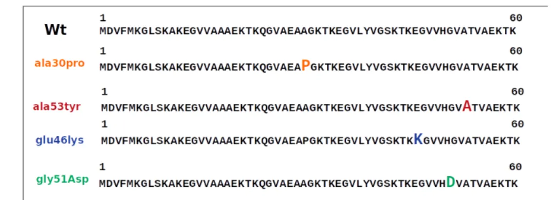
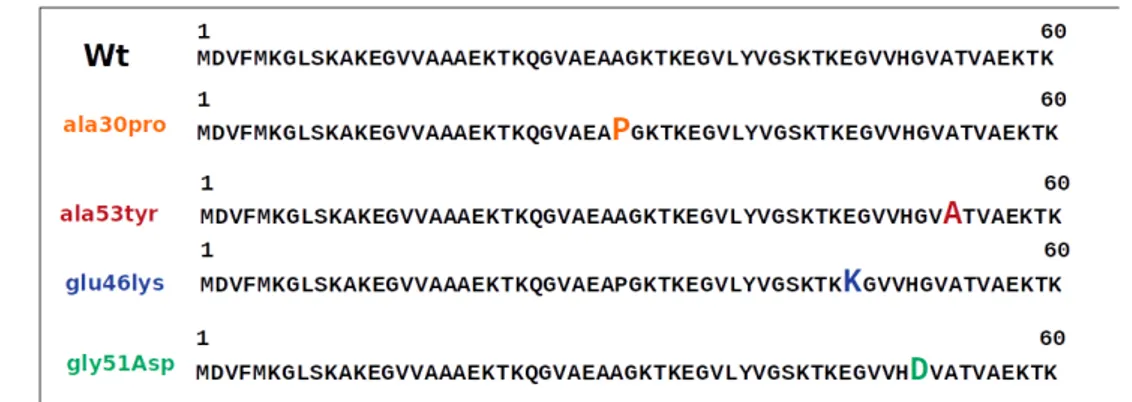
Fig.1.11shows the comparison between the wild - type (WT) primary sequence and that

of the mutants taken into consideration in this work, in order to highlight the position of

the point mutation. All mutations considered shown in Fig. 1.11 are in the N - terminus

and therefore in the figure only that part of the sequence has been reported.

Figure 1.11: Primary sequence of α-synuclein ’s mutants in comparison with WT sequence .

In Fig. 1.12 the substituted aminoacid (on top) and a schematic representation of the

Figure 1.12: Top: substituted aminoacid in the point mutation [11]. Bottom: schematic representation of α-syn sequence with the point mutation. Bottom figure

has been modified from Ref. [12].

The first effect caused by the mutations is the difference age in which the disease appears. The cases examined in this thesis are always faced with an early Parkinson disease, but in the literature also mutations that cause a delay in the appearance of symptoms are reported. The effects of these point mutations on the peptide aggregation kinetics have been widely studied. The A53T variant is considered to accelerate the aggregation, com-pared with the WT protein. The effects of A30P and G51D are instead under discussion, as it is reported both an increase and a decrease in the aggregation rate, while the effect of E46K is similar to that of the A53T but with a lower difference compared to the WT

protein [11,27].

By analyzing the A53T and A30P mutants with respect to the WT, it has been possible to evaluate their effect as a function of:

• Concentration of the protein; • β propensity.

The increasing of temperature, within a certain limit, causes an increase of aggregate structures. In fact, at low temperature all three types of proteins remain unfolded, while as the temperature increases, the mutants undergo a greater structural modifications compared to what happens in the WT protein. As far as the concentration effect is concerned, it is evident from literature that as the concentration of protein increases in solution, there is an increase in aggregation propensity. This increase is not the same for each mutant. The A53T mutant increases its propensity to aggregate more than the

A30T, which is however more inclined to from aggregate structure than the WT [27].

Looking at the content of β structures, FTIR measurements, shown in [27], show that

WT-α-syn results in an unfolded situation, while the A30P and A53T mutants, especially the latter one, show a greater presence of β structures.

The E46K mutant shows electrostatic properties similar to the WT protein, but exhibits, according to NMR measurements, conformational changes in the vicinity of the mutated amino acid, while the remaining part of the sequence does not present large conforma-tional changes. This mutant shows a greater capacity, compared to the WT, in the

formation of fibers, with a behavior very similar to the on of A53T mutant[28]. The

G51D mutation doesn’t affect the structure of free α-syn in solution and shows a slow aggregation rate in comparison with WT protein.

Small Angle Scattering

2.1

SAS: An introduction to the technique

The experimental technique applied in this thesis is Small Angle Scattering (SAS), which provide information on the structure of particles that have typical dimensions between

Angstrom (˚A) and Nanometers (nm). Depending on the probe used, X-Ray or

Neu-tron, this technique reveals differences in the electron scattering length density (SLD), proportional to the electron density, or in the neutron scattering length density, respec-tively. The IDPs experimental investigations carried out in this thesis have used the

the synchrotron’s X-Rays (Fig.2.1), using the Small Angle X-Ray Scattering’s technique

(SAXS).

In Fig. 2.2 the resolution of the SAS techniques is compared with other experimental techniques. It should be noted that while SAXS and SANS are investigating the same order of magnitude, they are sensitive to different characteristics of the sample.

Figure 2.2: Resolution of SAS technique

The application of SAS in Biology is very useful because with this technique is possible to investigate samples directly in solution. In the study of protein, SAS can provide information about:

• quaternary structure; • folded or unfolded status;

• conformational changes during the various active phases of the molecule; • unfolding processes due to chemical or temperature treatments under pressure;

• interactions between different macromolecules in solution; • hydration properties of macromolecules;

• kinetic process of protein aggregation.

The great advantage of SAS technique compared to others is that of being able to carry out the measurements in experimental conditions very similar to the in vivo environment and therefore to be able to study the macromolecules under different conditions of pressure, pH and temperature.

2.2

Small Angle Scattering geometry

The geometry of a SAS experiment is shown in Fig.2.3. A beam of X-Rays or Neutrons

impacts on the sample and this interaction generates the scattering phenomenon which is detected by a detector.

Figure 2.3: Schematic SAS experiment: A. Instrumental setup; B. Curve example. [13]

From a physical point of view, a SAS experiment can be schematized as in Fig.2.4.

q

incident beam

scat

tere

d be

am

k

k

2

θ

sample

The scattering process is considered elastic in first approximation. As shown in Fig.2.4,

k0 and k are the incident and diffuse wave vectors respectively while 2θ is the scattering

angle between the incident and the diffused vector. The scattering vector q is defined as:

q= (k − k0) (2.1)

and his modulus results:

q = 4π

λ sin θ (2.2)

where λ is the wavelength of the incident radiation and 2θ is the scattering angle. When the wavelength λ has been selected, for any 2θ angle at which the scattered ra-diation is detected we can associate its scattering wave vector q. From the Bragg’s law for X-ray Diffraction (XRD) of a crystal from a characteristic distance d between two of its planes we have nλ = 2d sin θ and substituting in the 2.2 is possible to deduce that in order to obtain information from the sample under study it is necessary to take into

account the minimum distance that can be detected that is: dmin ≈ 2π/qmax, qmax being

the maximum value of the scattering vector modulus.

Hence, in order to carry on a proper SAS experiment, it is necessary to roughly know the dimensions of the objects to be investigated, in order to appropriately choose the

distance between the detector and the sample that will determine the appropriate range of the modulus of the scattering vector (q-range).

2.3

SAXS Theory

In this section some basic concepts necessary for the use of this technique will be explained.

2.3.1

Macroscopic differential cross section

The SAXS technique makes it possible to measure the so-called macroscopic differential

scattering cross section, dΣ

dΩ(q), defined by the master equation:

dΣ dΩ(q) = 1 V ⟨ ⏐ ⏐ ⏐ ⏐ ∫ V dr ρ(r)eiq·r ⏐ ⏐ ⏐ ⏐ 2⟩ (2.3)

where V is the volume of the irradiated sample and the average is made on all

pos-sible positions and orientations of the particles in the system. Eq. 2.3 represents the

three-dimensional Fourier transform (FT) of the electron SLD, ρ(r), in the case of SAXS experiments, while for SANS ρ(r) indicates the neutron SLD. The scattering length den-sity ρ(r) can be expressed as:

where ρ0 is the average scattering density calculated on a larger volume than that

reso-lution volume. The fundamental equation therefore becomes:

dΣ dΩ(q) = 1 V ⟨_⏐ ⏐ ⏐ ⏐ ∫ V dr [δρ(r) + ρ0]eiq·r ⏐ ⏐ ⏐ ⏐ 2⟩ = 1 V ⟨ ⏐ ⏐ ⏐ ⏐ ∫ V dr δρ(r)eiq·r+ ρ0 ∫ V dr eiq·r ⏐ ⏐ ⏐ ⏐ 2⟩ (2.5) As 1

(2π)3 ∫ dr eiq·r it is a representation of the three-dimensional Dirac function, we will

have: dΣ dΩ(q) = 1 V ⟨ ⏐ ⏐ ⏐ ⏐ ∫ V dr δρ(r)eiq·r+ ρ0(2π)3δ(q) ⏐ ⏐ ⏐ ⏐ 2⟩ (2.6)

The contribute of the Dirac Delta is different from zero only for q = 0, therefore this term is not involved in a scattering experiment (q = 0 means that there was no diffusion). To formalize the presence of various diffusion centers within the sample and make explicit the term δρ(r), it is useful to define the dimensionless scattering amplitude of a particle:

Fi(q) = 1 fi ∫ Vi dr δρi(r) eiq·r (2.7)

where Vi is the volume of i-th particle that diffuses and fi is a normalization coefficient.

fi =

∫

Vi

dr δρi(r), (2.8)

Considering a system constituted by Np particles, with their center of mass in the vectors

position Ri and with orientation ωi with respect to the reference, each point k of the

particle will be identified by the vector rk = Ri+ uk (Fig. 2.5).

Figure 2.5: Representation of the position vector Ri.

The equation2.3 becomes:

dΣ dΩ(q) = 1 V ⟨_NP ∑ i=1 NP ∑ j=1 ∫ Vi ∫ Vj duidujδρi(ui)δρj(uj)eiq·(Ri−Rj)eiq·(ui−uj) ⟩ = 1 V NP ∑ i=1 f_i2 < F_i2(q) >ωi +1 V NP ∑ i=1 NP ∑ j̸=i fifj < Fi(q)Fj∗(q)eiq·(Ri−Rj)>ωi,ωj,Ri,Rj, (2.9)

where the first average is done on all possible orientations ωi of the particle i-th and the

second average is made on the combinations of orientations ωi e ωj and on the positions

Ri and Rj of the particles i and j. For the calculation of these averages it is useful to

introduce the distribution function related to the single particle P(1)_(ω

i) and the torque

distribution function P(2)(Ri, ωi, Rj, ωj) such that:

< Fi2(q) >ωi= ∫ dωiP(1)(ωi) Fi2(q) ∫ dωiP(1)(ωi) (2.10) < Fi(q)Fj∗(q)eiq·(Ri−Rj)>ωi,ωj,Ri,Rj= ∫ dωidωjdRidRjP(2)(Ri, ωi, Rj, ωj) Fi(q)Fj∗(q)eiq·(Ri−Rj) ∫ dωidωjdRidRjP(2)(Ri, ωi, Rj, ωj) (2.11)

The first term of the equation 2.9 describes the shape of the particle, while the second

term involves both the form and the correlation with other particles. This is why we define the average form factor the following term:

P (q) = ∑NP i=1fi2 < Fi2(q) >ωi ∑NP i=1fi2 (2.12)

and the structure factor this term:

S(q) = 1 + ∑NP i=1 ∑NP j̸=ififj < Fi(q)Fj∗(q)eiq·(Ri−Rj)>ωi,ωj,Ri,Rj sumNP i=1fi2 < Fi2(q) >ωi (2.13)

Obtaining:

dΣ

dΩ(q) = nP < (∆ρVP)

2_{> P (q)S(q), (2.14)}

where np is the average particle number density, NP/V , and < (∆ρVP)2>= _N1_P ∑Ni=1P fi2.

In this way we obtain a simple expression (2.14) that separates information about the

shape of the objects investigated and their correlations.

2.3.2

Two - states model

In most SAXS experiments on proteins we can consider each particle as an object with

uniform SLD, ρi, embedded in a solvent of homogeneous SLD ρ0. Working in very diluted

conditions, we can assume that ρ0 is the average SLD of the system. Hence in Eqs. 2.7

and 2.8 the function δρi(r) can be replaced by the constant ∆ρi = ρi− ρ0:

Fi(q) = 1 Vi ∫ Vi dr eiq·r (2.15) fi = Vi∆ρi. (2.16)

It can be shown that in the case of spherical particles with a uniform SLD, the expression of diffuse intensity becomes:

dΣ dΩ(q) = p ∑ α,β=1 √ nαnβ∆ρα∆ρβVαVβΦ(qRα)Φ(qRβ)Sαβ(q), (2.17)

where the form factor for a sphere of radius R is:

F (q, R) = Φ(qR) = 3sin(qR) − (qR) cos(qR)

(qR)3 . (2.18)

The structure factor is:

S(q) = ∑p α,β=1 √ nαnβ∆ρα∆ρβVαVβΦ(qRα)Φ(qRβ)Sαβ(q) ∑p α=1nα(∆ρα)2Vα2Φ2(qRα) . (2.19)

When we are dealing with even more diluted system (nα → 0),then we can approximate

the structure factor Sαβ(q) with the Kronecker delta function δα,β as we suppose that the

particles diffuse the radiation independently from each other. In the simplest case of a sample with a very diluted, monodisperse, two-phase and isotropic approximation, the diffuse scattering intensity reduces to:

dΣ

dΩ(q) = nP(∆ρ)

2_V2

where Vp is the single particle’s volume.

These approximations simply indicates that with the SAS technique it is possible to obtain information about the shape of the investigated object. Assuming different shapes,

corresponding form factors can be calculated. Some examples are shown in Fig.2.6.

Dumb-bellLong rod

Hollow sphereFlat disk

Sphere q (˚A) P (q ) 0.4 0.3 0.2 0.1 0 100 10−2 10−4 10−6 10−8

Figure 2.6: Examples of P (q) of particles with different shape [14]

2.4

Data analysis: fundamental approaches

In the following paragraphs some fundamental approaches in the SAXS data analysis will be explained.

2.4.1

Guinier approximation

It is possible to obtain information about the average size of a particle investigated by SAS by exploiting the Guinier approximation. This approximation starts from the

development of the average form factor according to the hypothesis of randomly oriented particles: < F2_{(q) >} ωq = 1 4π ∫ dωq 1 f2 ∫ VP ∫ VP dr1dr2δρ(r1)δρ(r2) eiq·(r2−r1) = 1 f2 ∫ VP ∫ VP dr1dr2δρ(r1)δρ(r2) 1 4π ∫ dωq eiq·(r2−r1) = 1 f2 ∫ VP ∫ VP dr1dr2δρ(r1)δρ(r2) sin (q|r2− r1|) q|r2− r1| . (2.21)

Developingsin x_x in a truncated Taylor series up to the second order and considering the

ori-gin of the coordinate axes in the particle’s SLD center in such a way that∫

VP dr δρ(r) rα = 0 where α = x, y, z, we obtain: < F2(q) >ωq = 1 − q2 3f ∫ VP dr r2δρ(r) + . . . (2.22)

At this point we can define in analogy with classical mechanics the gyration radius (Rg) of the particle respect to its center of SLD mass:

R2_g = 1 f ∫ VP dr r2δρ(r) = ∫ VP dr r 2_δρ(r) ∫ VP dr δρ(r) (2.23)

and then: < F2(q) >ωq = 1 − q2_R2 g 3 + . . . (2.24) ≈ exp ( −q 2_R2 g 3 ) (2.25)

This expression is known as Guiner’s law and coincides with the form factor for terms up to the fourth power of q. This relationship loses validity with an increase of q. It can be shown that the Guinier’s law is valid if the range of the exchanged wave vector is such

that q Rg < 1 − 1.3. The gyration radius of a particle can be directly associated to the

geometric characteristics of the sample. For example, for a sphere of radius R, we have

that R2

g = 53R2; for an ellipsoid of semi-axes A, B and C we have Rg

2

= (A2_{+ B}2_{+ C}2_)/5.

For other regular geometrical shapes, it is possible to determine a relationship between the gyration radius and the characteristic geometrical parameters of the i-th particle.

If in solution there are NP species of particles, the form factor becomes:

P (q) = ∑NP i=1fi2 ( 1 − q2R2g,i 3 ) ∑NP i=1fi2 + · · · = 1 −q 2_R2 g,a 3 + . . . ≈ exp ( −q 2_R2 g,a 3 ) , (2.26)

where the apparent squared gyration radius is weighted on the factors f2

i: R2_g,a = ∑NP i=1fi2R2g,i ∑NP i=1fi2 . (2.27)

In Fig.2.7 an example of Guinier’s plot is shown.

Figure 2.7: Guinier’s plot. Theoretical SAXS curves calculated using the SASMOL software [15] for two different globular proteins. The box shows the corresponding plot

made using the law of Guinier [14].

2.4.2

Kratky plot

Kratky’s plot is a particular graphical representation of experimental data that provides information on the compactness of the investigated object. The Kratky plot shows the

product dΣ_dΩ(q) q2 _{vs q. This representation is particularly useful for structural}

charac-terization of globular particles and for determining the different stages denaturing. In

Fig. 2.8 an example of Kratky’s plot from theoretical SAXS curve of different Bovinum

Serum Albumin (BSA) conformations is shown. In blue the typical bell-shaped trend of a globular protein is shown, red curve reports the trend of a molten - globule state and finally in black the trend of an unfolded protein is shown.

Figure 2.8: Kratky’s plot of theoretical SAXS curve of different BSA conformation [14]

Because the peak position of the Kratky’s plot is related to Rg of the objects in solution,

a variation of the position of the peak reflects a change in particles size. In particular,

the Rg increases if the peak of the Kratky’s plot moves to lower q. If the width and the

shape of the peak changes, it means that the object in solution is undergoing consistent structural changes.

2.4.3

Distance distribution function and Porod approximation

The Porod’s approximation, unlike the Guinier’s approximation, is useful for information on the volume and exposed surface of the particles in solution and is valid for large values of q. To derive the Porod’s approximation, it is firstly necessary to start from the expression of the form factor of the particle:

< F2(q) >ωq= P (q) =

∫ ∞

0

dr p(r) sin(qr)

qr , (2.28)

where p(r) is defined as the inverse isotropic Fourier transforms of P (q):

p(r) = 2r

π

∫ ∞

0

dq P (q) q sin(qr), (2.29)

with the normalization condition∫∞

0 dr p(r) = 1.

If we replace the equation2.21 with r = r2− r1, we obtained:

P (q) = 1 f2 ∫ VP ∫ VP dr1dr δρ(r1)δρ(r1+ r) sin(qr) qr = ∫ ∞ 0 drsin(qr) qr { 4πr2 1 f2 ⟨∫ VP dr1δρ(r1)δρ(r1+ r) ⟩ ωr } . (2.30)

In relation to the equation2.29 we deduce that we can express p(r) as:

p(r) = 4πr2 1 f2 ⟨∫ VP dr1δρ(r1)δρ(r1 + r) ⟩ ωr , (2.31)

showing that p(r) is related to the autocorrelation function of δρ(r). It can be shown

that the distribution function of distances p(r) it can also be used to determine the Rg

R2_g = 1 2

∫ ∞

0

dr r2p(r). (2.32)

For the two-phase model, the physical meaning of the p(r) can be elucidated. Indeed, if we replace the function δρ(r) with the contrast product δρ (which we assume to be constant) and of the function s(r) that describes the position and the shape of the particle (s(r) is equal to 1 if r is inside the particle, 0 if it is outside the particle), we have:

p(r) = 4πr2 1 V2 P ∫ VP dr1 < s(r1+ r) >ωr . (2.33)

It is clear that the p(r) represents the probability density to find a vector having the

first extreme on the point r1 of the particle and the second extreme still in the particle

and at a distance r from r1. If we develop the integral in the equation 2.33 considering

separately the particle (core) and the volume of an inner shell of thick r (which we call shell), we obtain: ∫ VP dr1 < s(r1+ r) >ωr = ∫ coredr1 < s(r1 + r) >ωr + ∫ shelldr1 < s(r1+ r) >ωr, (2.34)

The expression < s(r1+ r) >ωr= 1

4π∫ dωrs(r1+ r) represents the fraction of a solid angle

from which the point r1 can “see” the particle at a distance r. Hence, the argument of

the integral on the core of the particle is always 1 so that the value of this integral is

VP − SPr. For the integral on the inner shell we have:

∫

shelldr1 < s(r1+ r) >ωr = SP

∫ r

0

dx < s(x + r) >ωr, (2.35)

where SP is the particle’s surface and x is depth’s surface. Developing the integral on the

solid angle: ∫ VP dr1 < s(r1+ r) >ωr = VP − SPr + 3 4SPr = VP(1 − SPr 4VP ). (2.36)

Then the p(r) (2.33) becomes:

p(r) = 4πr 2 VP ( 1 −SPr 4VP ) + . . . at small value of r (2.37)

which can be inserted into the expression of the form factor 2.29 to study its trend, at

P (q) = 2πSP q4_V2 P +A(qrmax) q3_V2 P sin(qrmax) +B(qrmax) q3_V2 P

cos(qrmax) + . . . at large value of q. (2.38)

So the trend of the P (q) can be approximated by the Porod’s law:

P (q) ≈ 2πSP

q4_V2

P

. (2.39)

The approximation of Porod, with Guinier’s approximation, allow us to carry out a simple but appropriate analysis on a SAXS curve. The use of both approximations is to date the method of data analysis of SAS more common in literature.

2.5

SAS from PDB structures

It is possible to calculate the form factor P (q) starting from a structure deposited in the Protein Data Bank. Over the years, many methods have been developed to calculate the

SAXS or the SANS profile from a PDB file [29, 30] and in this thesis work the SASMOL

method was used. This method allows the determination of number and position of

water molecules in the first three hydration shells [15] and is able to calculate the protein

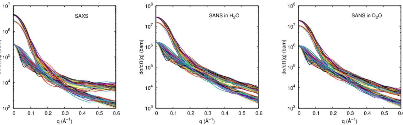
103 104 105 106 107 0 0.1 0.2 0.3 0.4 0.5 0.6 SAXS d σ /d Ω (q) (barn) q (Å−1) 103 104 105 106 107 108 0 0.1 0.2 0.3 0.4 0.5 0.6 SANS in H2O d σ /d Ω (q) (barn) q (Å−1) 103 104 105 106 107 108 0 0.1 0.2 0.3 0.4 0.5 0.6 SANS in D2O d σ /d Ω (q) (barn) q (Å−1)

Figure 2.9: Simulated curves on the conformational ensemble used in this work (Sec-tion 4.3) obtained using the SASMOL method

have different scattering length densities, according to the cosolvent distribution in the

local domain. In the figure 2.9 are shown some examples of the use of the SASMOL

method, applied to the ensemble used in this thesis work. Simulated SAXS curves (left panel), simulated SANS curves in water (center panel) and simulated SANS curves in a complete deuteration situation (right panel) are reported. It is important to note that the SASMOL method can also simulate SANS curves at different deuteration ratios. As you can see from the figure the scattering intensities are different by changing the type

of probe. The curves shown in the figure2.9 were made starting from the pdb structure

derived from [17], in which the ensemble consisted of three species (monomers, trimers

and tetramers of α-syn). This subdivision is in the plot of the simulated curves. This subdivision is evident in the simulated curves in which there are three different trends.

2.6

SAS of IDPs

In the last twenty years, IDPs have been discovered to be fundamental molecules in a

kind of protein has generated strong interest from researchers in order to understand the

structural bases of their functions [16]. Nuclear magnetic resonance (NMR) was the most

important structural biology technique used to characterize these structures at the level

of the primary sequence and to discover the most disordered regions of the sequence[31].

Despite the importance of the NMR technique, some structural characteristics relating to the size and overall shape of the IDPs or their complexes remain invisible to NMR

[16]. The best technique to obtain this information complementary to the NMR technique

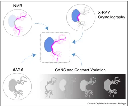
Figure 2.10: Representation of the structural sensitivity of NMR, X-ray crystallogra-phy, and SAS for a complex involving a IDP (central cartoon). NMR normally probes the flexible regions of these complexes while the globular partner and the interacting region remain invisible. Crystallography provides detailed information of the interact-ing region of the complex but not for the flexible parts. SAXS probes the complete ensemble, although the details cannot be assessed due to its inherent low-resolution. SANS, through contrast variation experiments, can probe independently both partners in the context of the complex depending on the deuteration level of the partners and the D2O/H2O of the buffer. SAS is an ideal tool to integrate NMR and crystallographic

in-formation to build complete structural and dynamic models of disordered biomolecular complexes [16].

Although SAS is a low-resolution technique, SAS curves do contain information on large-scale protein fluctuations and on the presence of multiple conformation in solution. The great challenge is to be able to interpret the SAS data in order to obtain useful struc-tural information despite the enormous conformational variability. In order to correctly interpret the structural information contained in SAS data it is necessary to use three-dimensional models. However, the generation of conformational sets of disordered pro-teins is extremely difficult, mainly due to the flat energy landscape and, consequently, to

numerical methods for generating three-dimensional IDPs models are based on

confor-mational landscapes derived from large databases of crystallographic structures [33]. The

principal limitation of these approaches is the lack of consideration of long-range interac-tions between distant regions of the proteins. To describe these characteristics, force fields are needed that take into account the interactions within the chain and the features of the solvent. The development of specific force fields to study conformational fluctuations

in IDPs is a very active field of research [34, 35]. Simulations of Molecular Dynamics

(MD) or Monte-Carlo (MC), with a precise description of the energy of the system, are

the best methods for correctly sampling the conformational space of these proteins [16].

As a matter of fact, the method developed in this thesis needs a conformational ensemble derived from computational results to interpret SAS data and be able to obtain, in this way, a description of the conformational behavior of the measured sample.

Experimental Data

3.1

SAXS - Experimental Data

The experimental data reported in this thesis have been recorded at the beam line BM29

at the European Synchrotron (ESRF) in Grenoble (Fig. 3.1).

Figure 3.1: The European Synchrotron Radiation Facilities, Grenoble, France

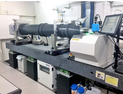
The beam line BM29 (Fig. 3.2) is a tunable energy beamline (from 7 to 15 keV) for SAXS experiments of biological macromolecule solutions with the goal to determine their

three-dimensional structures in a natural state with a “low” resolution (from nm to ˚A).

The achievable q - range is 0.0025 − 0.6 ˚A−1_{, which corresponds to the biggest measurable}

Rg of the investigated particle of ∼ 200 ˚A.

Figure 3.2: Beam Line 29 at The European Synchrotron Radiation Facilities, Grenoble, France

In the following paragraphs I will briefly illustrate the experimental sessions showing some SAXS curves recorded on α-synuclein samples.

3.2

α-synuclein

α-synuclein has been studied at different concentrations and at temperature of 25◦_{, 37}◦

in order to elucidate how a point mutation (Fig. 3.3) can modify the conformational landscape of this IDP.

Figure 3.3: Point mutation in α-synuclein primary sequence in comparison with WT.

For each sample a small amount of ∼ 30 µL has been inserted in the capillary. It was also measured the SAXS pattern of the buffer (PBS pH 7.4) to be subtracted from the

experimental curve. Figs. 3.4-3.8 shows some of the various curves recorded in different

10−4 10−3 10−2 10−1 0 0.1 0.2 0.3 0.4 d Σ /d Ω (q) (cm −1) q (Å−1₎ C=1.0 C=2.75 C=5.5 (a) 25◦_C 10−4 10−3 10−2 10−1 0 0.1 0.2 0.3 0.4 d Σ /d Ω (q) (cm −1) q (Å−1₎ C=1.0 C=2.75 C=5.5 (b) 37◦_C 10−4 10−3 10−2 10−1 0 0.1 0.2 0.3 0.4 d Σ /d Ω (q) (cm −1) q (Å−1₎ C=1.0 C=2.75 C=5.5 (c) 45◦_C

Figure 3.4: SAXS curve of WT α-synuclein

10−4 10−3 10−2 10−1 0 0.1 0.2 0.3 0.4 d Σ /d Ω (q) (cm −1) q (Å−1) C=0.7 C=3.1 C=6.1 (a) 25◦_C 10−4 10−3 10−2 10−1 0 0.1 0.2 0.3 0.4 d Σ /d Ω (q) (cm −1) q (Å−1) C=0.7 C=3.05 C=6.1 (b) 37◦_C 10−4 10−3 10−2 10−1 0 0.1 0.2 0.3 0.4 d Σ /d Ω (q) (cm −1) q (Å−1) C=0.7 C=3.05 C=6.1 (c) 45◦_C

Figure 3.5: SAXS curve of G51D α-synuclein mutant

10−4 10−3 10−2 10−1 0 0.1 0.2 0.3 0.4 d Σ /d Ω (q) (cm −1) q (Å−1) C=1.0 C=3.0 C=6.0 (a) 25◦C 10−4 10−3 10−2 10−1 0 0.1 0.2 0.3 0.4 d Σ /d Ω (q) (cm −1) q (Å−1) C=1.0 C=3.0 C=6.0 (b) 37◦C 10−4 10−3 10−2 10−1 0 0.1 0.2 0.3 0.4 d Σ /d Ω (q) (cm −1) q (Å−1) C=1.0 C=6.0 C=10.0 (c) 45◦C

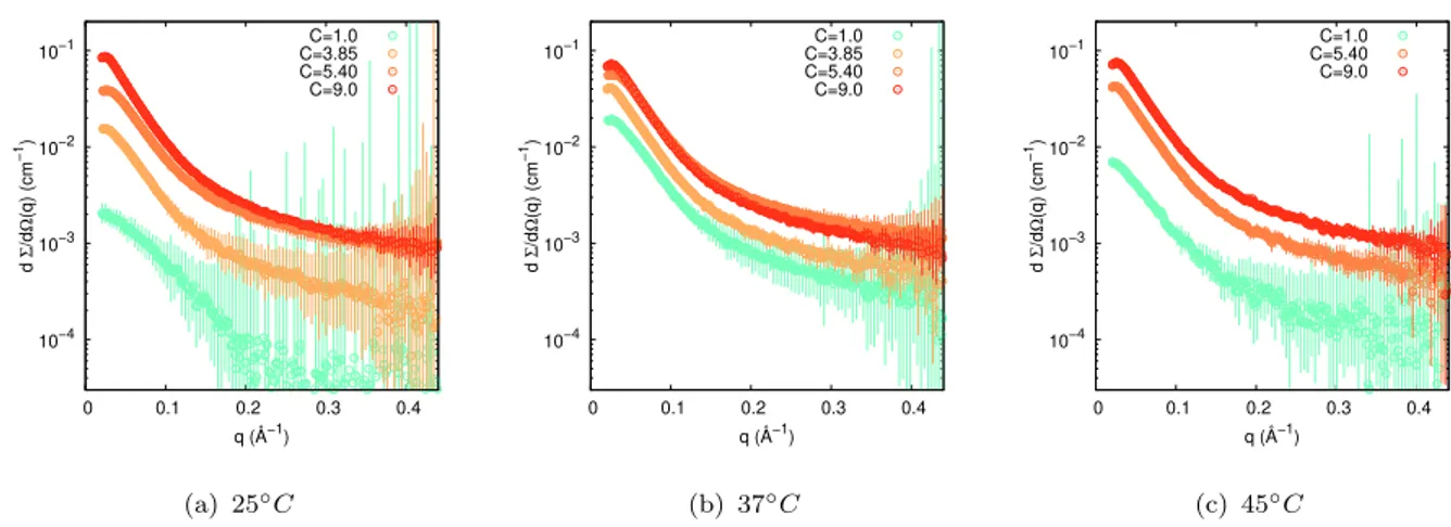
10−4 10−3 10−2 10−1 0 0.1 0.2 0.3 0.4 d Σ /d Ω (q) (cm −1) q (Å−1) C=1.0 C=3.85 C=5.40 C=9.0 (a) 25◦_C 10−4 10−3 10−2 10−1 0 0.1 0.2 0.3 0.4 d Σ /d Ω (q) (cm −1) q (Å−1) C=1.0 C=3.85 C=5.40 C=9.0 (b) 37◦_C 10−4 10−3 10−2 10−1 0 0.1 0.2 0.3 0.4 d Σ /d Ω (q) (cm −1) q (Å−1) C=1.0 C=5.40 C=9.0 (c) 45◦_C

Figure 3.7: SAXS curve of A53T α-synuclein mutant

10−4 10−3 10−2 10−1 0 0.1 0.2 0.3 0.4 d Σ /d Ω (q) (cm −1) q (Å−1) C=0.45 C=4.5 (a) 25◦C 10−4 10−3 10−2 10−1 0 0.1 0.2 0.3 0.4 d Σ /d Ω (q) (cm −1) q (Å−1) C=0.45 (b) 37◦C 10−4 10−3 10−2 10−1 0 0.1 0.2 0.3 0.4 d Σ /d Ω (q) (cm −1) q (Å−1) C=0.45 (c) 45◦C

Method

4.1

VBW methods: from SAXS to propensities

The overall goal of this work is the description of the conformational order/disorder of IDPs in terms of folding propensities of each aminoacid. The idea is to develop a method able to obtain information about IDPs structural features from a combination of computational results (e.g. a conformational ensemble) and SAS experimental data, as

introduced in Chapter 3. The focus of the method is the definition of propensity, that

will be defined in the next paragraphs. Firstly, it is necessary to define some fundamental aspects:

• definition of the conformational space; • availability of a conformational ensemble;

• availability of SAXS or SANS data to analyze (shown in Chapter3).

4.2

Conformational space

The first problem addressed in this methodological study has been to find a criterion for

dividing the space of the angles φ and ψ of Ramachandran [36] in regions that represent

the most significant conformational structures. For example, according to Ozenne et al.

[33] Ramachandran’s plot is divided into 4 regions defined as α-left, α-right, β-proline

and β -sheet, according to these relationships:

• αL (φ > O◦);

• αR (φ < O◦_{, −120}◦ _{< ψ < 150}◦_);

• βP (−100◦ _{< φ < O}◦_{, ψ > 50}◦_{, ψ < 120}◦₎

• βS (−180◦ < φ < −10O◦, ψ > 50◦, ψ < 120◦)

This choice seemed unrepresentative to us. Therefore the subdivision of the Ramachan-dran plan proposed in this thesis work was based on a probability distribution function of the φ and ψ angles obtained from a representative database of 500 structures present within the Protein Data Bank (http://kinemage.biochem.duke.edu/databases/top500.php). This database was created starting from 1000 protein structures and through the appli-cation of different structural analysis techniques the probability distribution p(φ, ψ) of the mediated conformations on all the residues of all proteins was generated. Using this

probability distribution function (Fig.4.1) the Ramachandran plot has been divided into

8 regions, obtained by cutting the p(φ, ψ) surface in the probability values of 0.0005 and

Figure 4.1: Probability distribution function from databases top500

The two-dimensional representation of the plot (Fig.4.2 4.3) was obtained with the use

of the Gnuplot software (http://www.gnuplot.info/ ).

Figure 4.2: Visualization of the two-dimensional regions obtained from the distribu-tion surface

The eight regions in which we decided to divide the plot are the 4 canonical regions in which there are the structures β, α-right, α-left and glicine zone, divided into energetically favorable, and energetically allowed, precisely as a function of the probability values with which the distribution was cut. Thus we have defined the following areas:

1. β favorable; 2. β allowed; 3. αR favorable; 4. αR allowed;