1
Strategic interaction and NFNE:
The case of
CO
2Concentration
By
Behnaz Minooei Fard
Supervisor:
Professor Giovanni Di Bartolomeo
2
Abstract (English)
Abstract
After the first formulation of optimal control problems in the middle of the 20th cen-tury, model predictive control (MPC) and nonlinear model predictive control (NMPC) gradually became popular methods in both science and industry. Considering the ad-vantages of NMPC as a practical method to solve dynamic decision problems numer-ically, this method could attract more attention in economics too. Later, in order to model strategic interactions between different policymakers, NMPC was extended to the NMPC feedback Nash equilibrium (NFNE).
With focusing on these novel and practical techniques, the aims of this thesis are con-sidered as follows. First, taking into account the privileges of mentioned techniques (NMPC and NFNE) such as repetitive solution of an optimal control problem in a receding horizon fashion and considering the time horizon, we use them in an envi-ronmental topic and assess the effects of different regimes on the climate change. Second, referring to the time horizon as a significant factor in these methods, we eval-uate the effect of “Different time horizons” on the results and finally, we extend the current NFNE method in order to have more accurate predictions, specifically where we face more than one state variable in our optimization problems.
3
In this thesis, we consider a significant climate issue as global warming. Since using non-renewable energy and as its result CO2 concentration leads to the negative
exter-nalities and affects individual welfare, for evaluating the interactions between differ-ent policymakers, we use a canonical growth model augmdiffer-ented with damages in the household’s welfare function. We assess the CO2 concentration level when players
operate under different regimes, in this thesis by different regimes, we refer to the cooperative and non-cooperative policies and we consider the period from 2019 to 2100. We start considering one common state variable as CO2 concentration and one
control variable as using non-renewable energy. Our result shows a big difference in the CO2 concentration level in the cooperative and non-cooperative situation.
Alt-hough, with cooperation between independent policymakers we can reach a lower level of externality but, still it is not the best emission pathway. However, if policy-makers find it difficult (e.g., for political reasons) to accept international binding agreements, and prefer to rely on their preferences for consuming non-renewal re-courses instead of considering the global warming, the negative externalities and dam-aging effects may be quite severe.
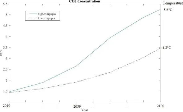
Moreover, along the line of Sims’s idea that agents often make decisions under infor-mation constraint, we interpret the finite horizon as a measure of inattention or myo-pia. When we apply different time horizons for introducing the policymakers’ myopia, we observe that interestingly, less myopic policymakers anticipate much less CO2
concentration above the pre-industrial level. However, results state that also if we find a way to remove policy uncertainty or constraints and have a more precise prediction (i.e., longer time horizon), still the result will not be satisfying by the year 2100.
Then, in our extended form of NFNE, we consider the transition from non-renewable to renewable energy as an important way to combat global warming. This transition
4
can also be considered as an additional instrument in cooperative situations. Hence, we suppose two state variables. Along with CO2 concentration which is the common
state variable, we take into account the capital stock to produce renewable energy. Also, we have two control variables as the extraction rate of fossil fuels and consump-tion. But, this extension in our model requires an extension in the method. So, we extend the current NFNE method and build two separate loops as two different games for optimization problems. These loops should be solved independently but simulta-neously to find those fixed points that players have no incentive to change that at each point of time. Results show that despite having the renewable resources, since there is not a suitable cooperation between countries/policymakers, we cannot expect to have a transition from non-renewable to renewable resources. But interestingly, if pol-icymakers accept a high degree of cooperation, we will reach really good results in CO2 concentration and eventually temperature.
5
Contents
Introduction ... 8
Chapter 1 ... 12
Nonlinear model predictive control theory ... 12
1.1 Fundamentals of Nonlinear model predictive control... 13
1.2 Continuous and Discrete Time Models ... 18
1.2.1 Timing assumptions ... 18
1.3 Advantages of NMPC ... 21
1.4 Alternative interpretations ... 24
Chapter 2 ... 26
NMPC Feedback Nash Equilibrium (NFNE) ... 26
2.1 Preliminary Definitions ... 27
2.2 Problem formulation ... 28
2.3 NFNE vs other differential games ... 32
Chapter 3 ... 35
Strategic Interactions and CO
2Concentration ... 35
3.1 An overview of global warming ... 36
3.2 Importance of CO
2concentration ... 37
3.3 Global warming as a global public good ... 39
3.4 Economic assessment models... 41
3.5 A two-country GPG-dynamic-provision game ... 43
3.5.1 Global mean temperature ... 46
3.6 The economic framework: CO
2Concentration ... 48
6
3.6.2 Policy equilibrium ... 51
3.7 Cooperative solution ... 52
3.8 Results ... 53
3.8.1 Calibration... 53
3.8.2 CO
2Concentration example ... 55
3.8.3 Non-cooperative VS Cooperative regime ... 56
3.9 Policymakers’ myopia ... 60
3.10 Concluding remarks... 62
Chapter 4 ... 64
Extension of NFNE method: Transition from non-renewable to
renewable energy ... 64
4.1 Related literature ... 65
4.2 Dynamic-provision game ... 67
4.3 Structure of NFNE with two state variables ... 69
4.4 The economic framework ... 74
4.5 The social planners’ problem and policy equilibrium ... 76
4.6 Results ... 78
4.6.1 Calibration... 78
4.6.2 Non-cooperative regime ... 79
4.6.3 Cooperative regime ... 81
4.7 Concluding remarks ... 84
Chapter 5 ... 86
Summary and Conclusions ... 86
7
A.1 Discretization ... 90
References ... 92
8
Introduction
Nonlinear model predictive control (NMPC) is an approach to solve dynamic decision models and it is applied to optimal feedback control of nonlinear systems. This method has some significant advantages. For example, it avoids gridding the state space, and considers finite horizon optimal trajectories in order to find the infinite horizon optimal trajectory. Also, comparing NMPC solution with other differential games such as open-loop and feedback Nash equilibrium, we can suppose that NMPC is a method using both open-loop and feedback information structures of the initial state value at the same time.
Furthermore, Di Bartolomeo et al. (2017) introduced an extension of NMPC called the NMPC feedback Nash Equilibrium (NFNE) which focuses on the length of fore-casting horizon. NFNE aims at modeling the strategic interactions between different policymakers. In this method, the procedure works in a loop consist of repeating the maximization/minimization of the optimal control problem to find an optimal strategy that players have no incentive to change it, at each point of time.
So, considering the efficiency of these methods in economics, at first, we have a com-prehensive review of the mentioned methods and their application in economics. Also, strategies, and equilibrium concepts both in the NMPC and NFNE will be discussed. In the next step, we use these novel methods in a climate change issue. In other words, using the mentioned techniques and considering different regimes, we aim at provid-ing a more precise prediction.
9
Global warming, as a controversial issue, is a result of raising in CO2 concentration.1
Due to the fact that CO2 emission has a high correlation with the consumption of fossil
fuels and this consumption increase rapidly, a large number of studies try to predict the level of CO2 concentration in the future and focus on mitigation policies in order
to combat global warming. But on one hand, most of the methods used before, have a deficiency related to the “Time Horizon” and this deficiency can be more prominent
when we notice that there is a big difference of the forecasting horizon between eco-nomics and climate issues. On the other hand, previous studies did not pay enough attention to this point that there are different policymakers who decide about these mitigations policies, not the United Nations and consequently it is about policymak-ers’ decisions to emit under cooperation or in a non-cooperative situation.
Considering global warming as a global public good which affects all countries, a significant question is how much CO2 concentration will be expected by emitting
un-der different regimes. Also, referring to the time horizon issue in NMPC and NFNE, on one hand, policymakers need, less information when making decisions because of using receding horizon solutions and on the other hand, we can assess the effects of policymakers’ short-termism on the predicted CO2 concentration level and the global
mean temperature. It is worth noting that shorter lengths in policymaker’s time hori-zons, can be associated with political economy or information constraints.2
Finally, we extend our research in two directions. At first, we extend NFNE technique to apply for the optimization problem with more than one dynamic, and then from the economic point of view, we take into account the ability to shift from polluting to
non-1 IPCC (2018).
10
polluting energy in order to have a more realistic view about our predictions. In the context of the transition from non-renewable to renewable resources, some studies have been done and renewable resources such as wind, water, solar, or nuclear energy are considered as a promising way to combat global warming. However, still there is an important question that if this transition will work efficiently, or it cannot bring enough incentives to encourage policymakers/countries to shift to these non-polluting energies. Hence, in this contribution, we extend the NFNE method and add another state variable to the previous economic framework called capital stock which is used to build the non-polluting energy resources.
In the end, it should be noted that models are coded and run in MATLAB in order to solve the optimization problems and simulates the responses of both economic and environmental variables under different regimes.
Outline and contribution
So, the remainder of this thesis is organized as follows:
Chapter 1 presents the Nonlinear model predictive control theory, optimization prob-lem, its advantages, and its application in economics.
In Chapter 2, we define the NFNE method and explore its difference with other dif-ferential games.
Chapter 3 using explained techniques, investigates the level of CO2 concentration
un-der different regimes by the year 2100, and strategic interactions. Also, we assess the effect of different forecasting horizons on the results.
11
In chapter 4, we have an extension of the previous method and framework. We con-sider two sources of energy as renewable and non-renewable and investigate the pos-sibility of transition between them.
Finally, Chapter 5 summarizes the major results as well as interesting topics that one could further investigate on.
12
Chapter 1
Nonlinear model predictive control theory
Nonlinear model predictive control (NMPC) is generally considered as an optimiza-tion-based method to solve dynamic decision models. This approach relies on iterative and finite-horizon optimization. It starts with implementing the initial value to the system and then repeatedly solves the original problem on a defined horizon by im-plementing the first element of the solution to the system.
In the middle of the 20th century, NMPC had developed from the theory of optimal control, and the first paper which was formulated the central idea of model predictive control was published by Propoi (1963). In the late 1970s, after a gap due to the inef-ficiency of computer hardware and software, MPC for linear systems and gradually,
13
NMPC which is applied to optimal feedback stabilization problems,3 became popular in control engineering and the industrial practice. However, after establishing success-fully in engineering, they were extended in economic applications too. The NMPC algorithm which we use today was published for the first time by Chen and Shaw (1982) and then after the basic principles of NMPC had been clarified, more advanced topics such as efficiency of numerical algorithms and robustness of stability had been done.
In this chapter, we introduce the concept of NMPC and then we describe the topic of time as discrete and continuous in this method. At the end, we explain the privileges of this method which make it different from other approaches.
1.1 Fundamentals of Nonlinear model predictive control
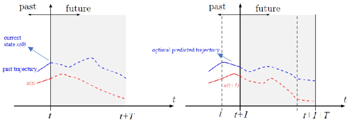
The aim of this technique is to predict future system behavior. Assume that we are given a vector of state variable 𝑥(𝑡) which has been influenced by a control input 𝑢(𝑡). We consider 𝑇 as the NMPC policy horizon also, the current state is sampled at time (𝑡) and the control problem will be optimized between 𝑡 and 𝑡 + 𝑇.
In order to predict future system behavior, we start with the most recent measurement of the state variable as the initial value 𝑥(0). we define a dynamical system to con-struct a prediction trajectory, 𝑥∗ (𝑡) as
14
𝑥(𝑡 + 1, 𝑥0) = 𝜑(𝑥(𝑡, 𝑥0), 𝑢(𝑡)) 𝑡 ∈ ℕ (1.1) 𝑥(0) = 𝑥0
Equation (1.1) describes how the state variable of the dynamical system develops un-der the influence of the control variable. The main idea of NMPC is that the control can be regularly adjusted and keep constant for a small finite interval. Hence, we as-sume that control variables are set at the beginning of each period and will be kept constant until its end.
Considering the above dynamic, we define the infinite horizon discounted optimal control problem by:
𝑉(𝑥0) = 𝑚𝑖𝑛 ∑∞ 𝛽𝑡
𝑡=0 𝑔(𝑥(𝑡), 𝑢(𝑡)) 𝑥(0) = 𝑥0 (1.2)
s.t. 𝑥(𝑡 + 1, 𝑥0) = 𝜑(𝑥(𝑡, 𝑥0), 𝑢(𝑡)) 𝑡 ∈ ℕ
The outcome of the optimal control problem is a vector of 𝑇 controls, 𝑢𝑡∗. We define the NMPC feedback as 𝜇(𝑥(𝑡)), and set 𝜇(𝑥(𝑡)) ≔ 𝑢𝑡∗(1), i.e., the first element of this sequence is the optimal NMPC at time 𝑡. NMPC does not want to involve an optimization over the entire planning horizon, but it involves the repetitive solution of an optimal control problem in a receding horizon fashion. Hence, in the next step, we use NMPC feedback, 𝑢𝑡∗(1), in the next sampling period. It should be noted that in the new step, the state variable is sampled between 𝑡 + 1 and 𝑡 + 𝑇 + 1, i.e., the prediction horizon keeps being shifted forward and because of this NMPC is called
15
receding horizon control. We will use the notation of prediction trajectory as 𝑥∗ (𝑡)
for a trajectory resulting from the control sequence 𝑢𝑡∗ and with the initial value 𝑥(0). Based on these definitions we can formulate NMPC solution algorithm.
Algorithm 1.1 (NMPC Solution Algorithm).
Given time horizon 𝑇; theini-tial condition of the dynamic system: 𝑥(0) = 𝑥0 . Consider a dynamic problem, e.g.,
(1.1) - (1.2). At each sampling time 𝑡 ∈ ℕ:
(1) Solve the following optimal control problem: 𝑚𝑖𝑛 ∑𝑇 𝛽𝑡
𝑡=0 𝑔(𝑥(𝑡), 𝑢(𝑡))
s.t. 𝑥(𝑡 + 1) = 𝜑(𝑥(𝑡), 𝑢(𝑡)) and 𝑥(0) = 𝑥0
and receive an optimal control sequence, 𝑢𝑡∗.
(2) Define the NMPC-feedback value 𝜇(𝑥(𝑡)) ≔ 𝑢𝑡∗(1) and apply it to the
system, i.e., 𝑥(𝑡 + 1) ≔ 𝜑 (𝑥(𝑡), 𝜇(𝑥(𝑡)))
(3) By repeating the above procedure, the prediction trajectory 𝑥∗ (𝑡) will be obtained.
This procedure leads to the infinite closed-loop trajectory 𝑥∗(𝑡), 𝑡 = 1, 2, 3, … along
with its control sequence, 𝑢∗ (𝑡), which consists of all the first elements of the optimi-zation sequences. In this method, we use open-loop finite horizon optimal trajectories, in order to find an infinite closed-loop prediction trajectory.
16
Above procedure is sketched in Figure. 1.1.
k jijii
Figure 1.1 Illustration of the NMPC
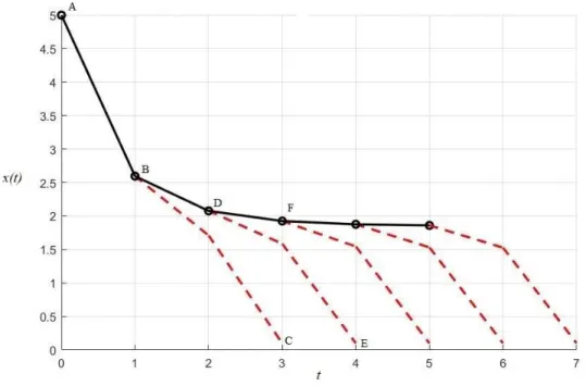
Example 1.14 Consider a simple growth model as 𝑓(𝑥(𝑡), 𝑢(𝑡)) = ln(𝐴𝑥𝛼− 𝑢)
s.t 𝑥(𝑡 + 1) = 𝑢(𝑡)
Where 𝐴𝑥𝛼 is a production function and 𝑥 is the capital stock. Solution will be reached by:
𝑉(𝑥) = 𝐵 + 𝐶 ln 𝑥, with 𝐶 𝛼 1−𝛼𝛽 and 𝐵 = ln((1−𝛼𝛽)𝐴)+ 𝛽𝛼 1−𝛽𝛼ln (𝛼𝛽𝐴) 1−𝛽 4 Grüne et al. (2015).
17
If initial value 𝑥(0) and policy horizon 𝑇, are set equal to 5 and 3 respectively and 𝛼 = 0.34, 𝛽 = 0.95 and 𝐴 = 5, then the optimal solution is:
𝑢∗ (𝑡) = (2.59,2.07,1.92,1.87,1.85) .
In figure 1.2, we see the first open-loop optimal trajectories (dashed) as A-C which is a vector of 3 controls. Then, by picking up the first element of this vector and applying it to the system, point B has been reached. B is the value of the state variable for the next step 𝑥(1).
Figure 1.2 Open-loop optimal trajectories (dashed) and Closed-loop trajectory (solid)
18
1.2 Continuous and Discrete Time Models
Basically, NMPC is applying in discrete-time problems. However, we usually face with time models in form of differential equations. Hence, the continuous-time problems need to be discretized in continuous-time in order to apply in this method.5 In the following, we define how we can convert any continuous-time model into dis-crete-time model. But at first, we describe the timing assumption that we are going to use in the current thesis.
1.2.1 Timing assumptions
We can consider a continuous-time models in general, or a particular time assumption. In this thesis, we are going to use a mixed-time-structure model.
Assume that we have the infinite horizon discounted optimal control problems in con-tinuous time where 𝑡 ∈ ℝ0+
𝑉(𝑥0) ≔ 𝑚𝑖𝑛 ∫ 𝑒∞ −𝜌𝑡 𝑔(𝑥(𝑡), 𝑢(𝑡))𝑑𝑡
0 (1.3)
𝜌 is the discount rate 6 and
𝑥(𝑡 + 1) = 𝜑(𝑥(𝑡), 𝑢(𝑡)), 𝑥(0) = 𝑥0 (1.4)
5 Grüne et al. (2015).
19
We consider a specific time structure as a mixed-time-structure model where state variables evolve in a continuous-time, i.e., 𝑡 ∈ [0, ∞), whereas controls are constant in the interval Δ, which occurs between 𝜏 − 1 and 𝜏 .
This happens because policymakers set their controls in a discrete fashion (policy in-struments are set at 𝜏 ∈ ℕ). In other words, the state variable 𝑥(𝑡) is evolved in con-tinuous time while the control ones 𝑢(𝑡) can be regularly adjusted and kept constant
for Δ.7
So, the assumption needs to implement as a receding horizon solution, but it is without loss of generality since Δ can be arbitrarily small. Here, it is worth noting that for simplicity, we assume control variables are set at the beginning of each period. We assume Δ = 1 and for any 𝑥 ∈ ℝ0+, we indicate 𝑐𝑒𝑖𝑙(𝑥) and 𝑓𝑙𝑜𝑜𝑟(𝑥) by ⌈𝑥⌉ and ⌊𝑥⌋, respectively. Then we define 𝜏 = ⌈𝑡⌉.
Fig. 1.3 can clarify the above notion.8 For instance, we can see that 𝜏 = 1 for any 𝑡 ∈
[0,1) or 𝜏 = 6 for any 𝑡 ∈ [5,6) and because of our small supposed interval (Δ = 1) it can be interpreted as continuous-time while we should notice that control variables used in each period have been set at the beginning of that period.
7 Di Bartolomeo et al. (2017). 8 Grüne and Pannek (2011).
20
Fig 1.3 The sequence at 𝑢(𝑡) on the left corresponds to the constant control functions with 𝑢(𝜏) = 𝑢(𝑡) for almost all at 𝑡 ∈ [𝜏 − 1, 𝜏)
Considering the above explanation, NMPC in continuous-time or mixed-time-struc-ture can be defined as follows.
Definition 1.1 (NMPC Solution, mixed-time-structure)
Given the initial condition of the dynamic system: 𝑥(0) = 𝑥0 ,defining the vector of policies between 𝑡 and 𝑡 + 𝑇 as 𝑢𝑡 ∈ ℝ𝑇 and 𝑢(𝜏) = 𝑢(𝑡) for almost all at 𝑡 ∈ [𝜏 −
1, 𝜏) :
NMPC feedback solution is a sequence {𝑢∗(𝑡)}1∞ such that each element is 𝑢∗(𝑡) =
𝑢𝑡∗(1), where policymaker aims to maximize/minimize
𝐿𝑡(𝑢𝑡) = ∑𝑡+𝑇𝜌𝜏−1
𝜏=𝑡 ∫ 𝑔(𝑥(𝑡), 𝑢𝑡(𝜏))𝑑𝑡 𝜏
𝜏−1 ,
21
Hence, during the time, economy evolves according to the following differential equa-tion
𝑥̇(𝑡) = 𝑓(𝑥(𝑡), 𝑢∗(𝑡)) (1.5)
And the policymaker aims to optimize the following inter–temporal loss/benefit:
𝑉(𝑥0) = ∑∞ 𝜌𝜏−1
𝜏=1 ∫ 𝑔(𝑥(𝑡), 𝑢(𝜏))𝑑𝑡 𝜏
𝜏−1 (1.6)
Where 𝜌 is the discount factor.9
So, given a dynamical system i.e. (1.5) and according to the above definitions, we can use the basic NMPC algorithm (1.1) in our mixed-time-structure model.
To solve the optimal control problem in continuous-time numerically, we need to con-vert it to the optimal control problem in discrete-time. For this purpose, it needs to be discretized in time in order to apply in the NMPC method. Hence, we use the first step of semi–Lagrangian discretization technique which is in time.
In Appendix A, it is explained that how we are able to solve the optimal control prob-lem in the NMPC algorithm numerically, by illustrating the discretization technique.
1.3 Advantages of NMPC
The first important advantage of NMPC is considering as the policymakers’ time ho-rizons. The time horizon is strongly related to the two different arguments. The first refers to the different time perspectives for different policymakers because of policy
22
uncertainty or policy constrains. The second argument refers to the limited capabilities of policymakers in order to forecast the effect of their policies and/or the policies of other policymakers. This limitation is the direct result of making decisions under lim-ited information. Shorter horizons can be interpreted as the measure of short-termism.10 This bounded rationality also was discussed by Simon (1957) and Forte (2012). Forte believes that the public choice approach is fundamentally micro-eco-nomic and is based on limited rationally.
Sims (2005, 2006) showed that agents make decisions under limited information which might be
a) the result of not available information.
b) imprecise answers to available information.
According to the Sims, with increasing the agents’ information and information pro-cessing capacity this limitation can be solved and better approximation for infinite trajectory will be possible.
We can deal with these constraints, referring to the main principles of NMPC. As we explained, we compute finite horizon optimal trajectories in order to find the infinite horizon optimal trajectory so, in the NMPC compared with the other infinite horizon models, agents need, less requirement of information when making decisions. In other words, we make a decision for the control of the next step by looking at the problem on a shorter time horizon.
Another significant advantage of NMPC is that this method is one of the most ad-vanced control approaches for multi-dimensional systems. In this approach, state and
23
control constraints allow us to consider more complex dynamics due to the less pos-sibility for solutions to stick in dimensionality trap. NMPC only computes one optimal trajectory at a time, therefore, it avoids to grid the state space. For this reason, the computational demand grows much more moderately with the space dimension.11 It is worth noting that the principles of NMPC can also create a deficiency for this method. As we explained in the NMPC procedure, we start from the current state 𝑥(0) and only the first decision step is implemented, however the given control sequence will be 𝑢(0), . . . , 𝑢(𝑇 − 1). So, considering the policy horizon 𝑇, in the closed-loop solution we are always 𝑇 − 1 periods away from the final decision. It refers to the point that, we never can see the effects which appear at the end of the policy horizon. According to Grüne, et al. (2015) for this problem, in the shorter decision horizon we can use the salvage value which can be determined in a reasonable way.
This deficiency implies that the optimization horizon 𝑇 plays a significant role in this method because there is a tradeoff between good approximation of 𝑇 and numerical accuracy. This tradeoff happens because on one hand, we can expect a good approxi-mation of the infinite horizon optimal trajectories when the optimization horizon is sufficiently large, but on the other hand, large horizons increase the decision horizon and it may lead to the dimensionality and numerical problems. So, the length of the time horizon should be considered in NMPC precisely.12
Considering explained advantages, NMPC can be considered as a practical option to solve dynamic decision problems numerically, in order to find global solutions. This approach can be useful in different economic areas such as economic growth and
11 Grüne et al. (2015).
24
ecosystem management, when we face a more complicated dynamic while using com-monly numerical techniques for solving them are difficult. Moreover, the possibility of using NMPC to solve nonlinear dynamic decision problems, both continuous and discrete-time models and considering regime changes makes this technique attractive in economics.
1.4 Alternative interpretations
Short-termism which is the result of uncertainties of policymakers, can be interpreted as “policymakers’ inattention” or “myopia”. Bounded rationality which was
formal-ized in NMPC by Grüne et al. (2015) and Di Bartolomeo et al. (2017) refers to this notion. Since NMPC optimization involves the repetitive solution at each sampling of time, instead of the entire planning horizon, in the context of bounded rationality, a shorter horizon can be interpreted as measuring stronger inattention.13
In this context, some notable researches have been done. For instance, Di Bartolomeo et al. (2017) focused on pollution regulation policies and inattention. They found that inattention basically affects the transition dynamics and it leads not only to quicker, but also more costly, transitions. Moreover, their results show that inattention may accelerate climate change by under-evaluating the environmental cost.
Also, referring to this fact that policymakers generally are stuck in time, Di Bar-tolomeo et al. (2018) used inattention as “policy myopia”. They tried to distinguish
25
the effects of policymakers’ time horizons on debt stabilization. According to their
results policy myopia induces policymakers to be more aggressive in stabilizing the debt at the beginning, but it is less effective in reducing excessive public debts in the long run.
In this thesis, we consider different policy horizons in order to investigate the effect of policymakers’ myopia on climate change.
26
Chapter 2
NMPC Feedback Nash Equilibrium (NFNE)
In this chapter, we want to define a novel concept as the NMPC feedback Nash Equi-librium (NFNE).NFNE is the extended form of NMPC and it is modeling the strategic interactions between different policymakers. This method proposes the results with feedback structure in an infinite horizon control problem. It is worth noting that NFNE as well as NMPC is related to the bounded rationality and inattention. We start with the definition and notion of NFNE and then describe the interaction between policy-makers. Furthermore, we make a comparison between NFNE and other differential games.
27
2.1 Preliminary Definitions
Di Bartolomeo et al. (2017), with focusing on the length of the forecasting horizon, introduced NFNE. This method which applies the NMPC technique to differential strategic games, is the combination of the NMPC method in economics, proposed by Grüne et al. (2015), and moving horizon LQ–control in dynamic games, used by Van den Broek (2002). In order to solve problems involving multiple interacting agents, they formalized an equilibrium concept as the NMPC Feedback Nash Equilibrium and developed a routine to compute it. Their work can be used in different areas such as environmental economics, industrial organizations, decision and management sci-ence, marketing, and quantitative methods.
NMPC is a method which let policymakers to predict the effects of their actions and/or their opponent’s actions on a finite receding horizon. Moreover, the length of the
fore-casting horizon can be interpreted in two ways: first, as a specific aspect of bounded rationality, second, with regard to different policymakers that may have different time perspectives.
In the NFNE method, the policy equilibrium is obtained by applying nonlinear model predictive control techniques to differential strategic games. It means that policymak-ers’ problems involve the repetitive solution of an optimal control problem at each
instant of time. But since we consider strategic interactions – differently from the usual NMPC solution – players interact in each instant of time in an infinite time setting and they try to predict the dynamics and the opponents’ moves during a given
time horizon. Each player works along a receding horizon strategy and the same as the NMPC, when a vector of control variables is calculated, only the first element will be used. Each of the optimal control problems must result in an open-loop Nash
28
equilibrium. So, Di Bartolomeo et al. (2017) referred to this kind of equilibrium as Non-linear model predictive control Feedback Nash Equilibrium (NFNE).
2.2 Problem formulation
In this section, we describe the basic principles of the NFNE. As we mentioned before, for a given time horizon, NFNE allows one to predict the dynamics of decision vari-ables of the other players in each instant of time. For the sake of simplicity, we sup-pose the case of two players.
Hence, the economy evolves according to the decisions of two policymakers 𝑖 ∈ {1,2} based on the following differential equation:
𝑥̇(𝑡) = 𝑔(𝑥(𝑡), 𝑢1(𝑡), 𝑢2(𝑡)) (2.1)
Equation (2.1) describes how the state 𝑥 of a dynamical system evolves in time 𝑡 un-der the influence of both the control 𝑢1 and 𝑢2.
And, both players want to minimize(maximize) the loss(benefit) such as:
𝑉𝑖(𝑥0) = ∑∞𝜏=1𝜌𝜏−1 ∫𝜏−1𝜏 𝑔𝑖(𝑥(𝑡), 𝑢𝑖(𝜏), 𝑢−𝑖(𝜏))𝑑𝑡 (2.2) Where 𝜌 is the discount rate.
Same as NMPC, we assume that policymakers’ optimal problems involve the repeti-tive solution of a receding horizon fashion, instead of over the entire planning horizon.
29
Since we assume that their problem is a Nash equilibrium in each instant of time, so we should find an optimal strategy in which players have no incentive to change their policies.
Using the definition of NMPC we can define the NFNE as follow:
Definition 2.1 (NFNE)
Given the initial condition of the dynamic system:𝑥(0) = 𝑥0 , and the control of the other player, defining the vector of policies between
𝑡 and 𝑡 + 𝑇 as 𝑢𝑡∈ ℝ𝑇 and 𝑢(𝜏) = 𝑢(𝑡) for almost all at 𝑡 ∈ [𝜏 − 1, 𝜏) and two poli-cymakers as 𝑖 ∈ {1,2} :
NFNE feedback solution is a sequence of two elements 𝑢1∗(𝑡), 𝑢2∗(𝑡) }1∞ where
𝑢𝑖∗(𝑡) = 𝑢𝑖t (1) and 𝑖 ∈ {1,2} i.e., the first element of each sequence is the optimal
NFNE at time 𝑡 and Policymaker aim to maximize/minimize
𝐿𝑡𝑖(𝑢𝑡) = ∑𝑡+𝑇𝜌𝜏−1
𝜏=𝑡 ∫ 𝑔𝑖(𝑥(𝑡), 𝑢𝑖𝑡(𝜏), 𝑢−𝑖𝑡 (𝜏))𝑑𝑡 𝜏
𝜏−1 𝑖 ∈ {1,2}
s.t. 𝑥̇ = 𝑓(𝑥(𝑡), 𝑢𝑖(𝜏), 𝑢−𝑖(𝜏) }1∞) 𝑡 ∈ ℝ0+, 𝜏 ∈ ℕ
Hence, during the time, economy evolves according to the following differential equa-tion
𝑥̇(𝑡) = 𝑔(𝑥(𝑡), 𝑢1∗(𝑡), 𝑢2∗(𝑡)) (2.3)
and policymakers aim to optimize the following problem:
𝑉𝑖(𝑥0) = ∑∞𝜏=1𝜌𝜏−1 ∫ 𝑔𝑖(𝑥(𝑡), 𝑢𝑖(𝜏), 𝑢−𝑖(𝜏))𝑑𝑡 𝜏
𝜏−1 𝑖 ∈ {1,2}
30
NFNE includes the strategies that players have no incentive to change them at each period of time 𝜏 and it is explained by the optimal strategies 𝑢1∗(𝜏) and 𝑢2∗(𝜏), as:
𝑁𝐹𝑁𝐸 ∶= {𝑢1∗(𝜏), 𝑢2∗(𝜏)}, ∀𝜏∈ ℕ (2.4)
Hence, given a dynamical system i.e., (2.3) and according to the above definitions and the algorithm1.1, we can find the prediction trajectory and optimal strategies, 𝑢1∗(𝜏) and 𝑢2∗(𝜏), via algorithm 2.1 as follows.
Algorithm 2.1 (NFNE).
Considering the first period 𝜏 = 1, given time horizon𝑇, the initial condition of the dynamic system: 𝑥(0) = 𝑥0 and an initial guess for the policy of player 2, optimal strategies of two countries will be found as follows:
(1) Solve optimal control problem of first player between 1 and 𝑇:
𝑚𝑖𝑛 𝑉𝑖(𝑥0)
s.t. 𝑥̇(𝑡) = 𝑔(𝑥(𝑡), 𝑢1(𝑡), 𝑢2(𝑡)) The outcome is a vector of 𝑇 controls, 𝑢̃1.
(2) Then, using the result vector as the guess for the policy of the first player, i.e., 𝑢1 = 𝑢̃1 (obtained from step (1)) and 𝑥(0) = 𝑥0, then we should solve the
op-timal control problem for player 2 between 1 and 𝑇,
𝑚𝑖𝑛 𝑉−𝑖(𝑥0)
31
Again, the outcome is a vector of 𝑇 controls, 𝑢̃2.
(3) Repeat step 1 and 2 using 𝑢̃2 for the first player and new 𝑢̃1 for the second
player, which are resulted by the optimization process, until a fixed point is found, i.e. vectors 𝑢1𝑜(1) and 𝑢2𝑜(1).
(4) At this point, we take the first elements of vectors 𝑢1𝑜(1) and 𝑢2𝑜(1), which are
the optimal NFNE at time 𝜏 = 1, i.e., 𝑢1∗(1) and 𝑢2∗(1). And then by applying
the optimal NFNE solution in usual dynamic, 𝑥̇(𝑡) = 𝑔(𝑥(𝑡), 𝑢1(𝑡), 𝑢2(𝑡)) we obtain 𝑥∗(1).
(5) Then, having 𝑥∗(1) and using 𝑢2𝑜(1) as the guess vector for the policy of
player 2, repeat the same procedure as just described in order to find e.g. 𝑢1∗(2) and 𝑢2∗(2)….
(6) The optimal policy vectors 𝑢𝑖∗(𝑡), 𝑖 ∈ {1,2} , are found by repeating the proce-dure just described.
Above algorithm is generalized to two players, hence dynamic for 𝑥(𝑡) is implied by NFNE as:
𝑥̇ = 𝑓(𝑥(𝑡), 𝑢1∗(𝜏), 𝑢2∗(𝜏)) for in 𝑡 ∈ ℝ 0
32
Based on the above explanation we can say that the NFNE technique can be used in the games as a novel technique where we want to predict the dynamics of other play-ers.
2.3 NFNE vs other differential games
In this section, we want to describe the advantages of NFNE as a prediction method and investigate the differences between NFNE and other differential games.
Differential games can be used widely in economic problem analysis and in dynamic games. It should be mention that in dynamic games, information that is available for the player is a significant issue because it leads to the different strategies adopted by players and different game situations.
Hence, in order to describe the game, at first, we need to identify the available infor-mation at each time 𝑡. For instance, while open-loop solution depends on time and initial state of the system, feedback controls depend on time and current state.14 In the
former game, players are just aware of the initial state, the game structure and they determine their actions for the entire planning horizon before the process starts. Whereas, in the latter one, players are allowed to observe at every point in time the current state of the process and determine their actions based on this observation.15
14 Ngendakuriyo, (2010). 15 Basar and Olsder (1982).
33
Comparing NFNE with these two differential games (i.e., Open-loop and Feedback Nash Equilibrium) NFNE solution also depends on time but, if we consider infor-mation structures, NFNE is a method using both open-loop and feedback inforinfor-mation structures at the same time. In other words, as we explained before NFNE is a receding horizon strategy which means that at each instant of time the horizon is moving toward the future, using the first control signal of the sequences calculated at previous steps. Hence, at the beginning of each period, the initial state variable is fixed over the time interval but once we apply the new control variable resulted from the optimization, a new measurement of initial state variable appears and it will be used for the next pe-riod. So, each player plays a non-cooperative strategy in each iteration and uses the most valid information at each instant of time to predict the future.
Moreover, in NFNE – as an extended form of NMPC – we do not need to the lineari-zation techniques to solve nonlinear dynamic problems globally. Also, in this tech-nique, by adding state and control constraints and by having a sufficiently long time horizon, we avoid difficulties of nonlinear games such as multiple equilibria.
In this thesis, we aim at using NMPC and NFNE in the environmental context under different regimes i.e., cooperative and non-cooperative. Considering the climate issue, we need to be concerned with a long time horizon of centuries while, in the context of economics, in the best case, we have the prediction only for a few decades which means that policymakers in these two fields have different time perspective. So, using a receding horizon method which also does not have the difficulties of other nonlinear games, can provide better predictions in the environmental issues. However, to reach
34
our purpose, we should extend the current NFNE method which before has been ap-plied only for the models with one state variable.16
35
Chapter 3
Strategic Interactions and CO
2Concentration
Considering the privileges of NMPC and NFNE, in this chapter we use the explained techniques in an environmental topic. We start with investigating the CO2
concentra-tion level, under different policy regimes. In this thesis, by different regimes, we refer to the cooperative and non-cooperative polices. For this purpose, we use a canonical growth model which is augmented with damages in the welfare function. Compared with other assessment models, this approach ties economic activity with externalities and feedback effects. Our primary goal is not to evaluate different abatement policies, but we want to study the interaction between different policymakers under different strategies. Then we investigate the effect of policymakers’ myopia on the results and assess how different time horizons can change the result.
36
3.1 An overview of global warming
Nowadays, global warming is considered as one of the most controversial issues and it has recently attracted considerable scientific and policy attention. Considering the importance of global warming, at first, we need to figure out the reason of this climate change. According to a large number of studies, the main reason has been recognized as raising in greenhouse gases (GHGs) concentration, and specifically Carbon dioxide (CO2).
Before the industrial revolution, it was a balance between inflows of GHGs and out-flows of carbon absorbed by ocean and plants but increasing the use of fossil fuels including coal, natural gas, and oil are recognized as the main human activities which changed that balance and led to the CO2 emission by more than 3% per year on average
in the 2000s.17 These human activities have made approximately 1.0°C of global warming above pre-industrial level and if we continue to emit at the same current rate it is ‘likely18 with high confidence’ to reach 1.5°C between 2030 and 2052.19
According to the United States Environmental Protection Agency (EPA), in 2017, CO2 emissions from fossil fuel combustion, were the largest source of GHGs
emis-sions – with about 76% of total Global Warming Potential (GWP)20 – and it was
17 Garnaut (2011).
18 ‘Likely’ refers to the level of confidence: ‘66–100%’. 19 IPCC (2018)
20 Global Warming Potential: The cumulative radiative forcing effects of a gas over a specified time
horizon resulting from the emission of a unit mass of gas relative to a reference gas. The GWP-weighted emissions of direct greenhouse gases in the U.S. Inventory are presented in terms of equivalent emis-sions of carbon dioxide (CO2).
37
accounted for all the US. It should be mentioned that although emissions from other sources, e.g., industrial processes, agriculture, waste, land use, land-use change and forestry are also significant, they are not included in these estimations due to some reasons such as lack of data availability, higher level of uncertainty in quantification methods, and smaller contribution to total emissions.
Hence, in this thesis, we concentrate on the cumulative global emissions of CO2 as a
significant part of GHGs and the energy sector and specifically in this chapter, we investigate the level of CO2 concentration and global mean temperature, under
differ-ent policy regimes.
3.2 Importance of CO
2concentration
Externalities and negative effects of CO2 concentration not only affect the present but
also the future. So, in order to limit global warming, we need to limit the total cumu-lative global emissions of CO2 since the pre-industrial period. Scientific evidence
shows that before the Industrial Revolution, the global average amount of CO2 was
about 280 parts per million (ppm), however the average CO2 concentration in
Decem-ber 2018 has been recorded around 408 ppm.21 According to the IPCC (2018), emis-sions scenarios that limit the concentration level, up to 450 ppm are likely to achieve
21 Dr. Pieter Tans, NOAA/ESRL (www.esrl.noaa.gov/gmd/ccgg/trends/) and Dr. Ralph Keeling,
38
2°C above pre-industrial temperatures while, scenarios that reach CO2 concentration
of 650 ppm will lead to 3°C by 2100 with the same level of confidence.
Hence, different actions have been proposed by researchers in order to limit climate change. These efforts generally elaborate on subjects such as mitigation policies e.g., carbon tax and cap and trade. However, it should be noted that climate policies usually imply tradeoffs at the domestic level and externalities at the international one, which makes their implementation difficult because on one hand, policymakers need to do an immediate action to control the climate change and on the other hand, any attempt to reduce CO2 emissions (as the main factor) such as reduction in the use of fossil
fuels, transition from fossil fuels to renewable energy and new technologies would be economically costly22 and may lead to changes in major economic issues such as pro-duction, consumption, and investment. These tradeoffs refer to a fact that govern-ments prefer to set the plans for national emissions according to their national inter-ests, i.e., under non-cooperative situations, and because of these preferences still world community is struggling to achieve an effective international agreement in or-der to reduce CO2 emission. We can refer to some of the most significant meetings
and commitments about the climate change as Kyoto (1997), Copenhagen (2009), Doha (2012), Warsaw (2013) and Paris (2015). However, theses international negoti-ations generally face difficulties and these difficulties show that global warming is considered as a case of global public good (GPG).
39
3.3 Global warming as a global public good
Global warming is considered as a polar case of Global Public Good (GPG). An im-portant point about global public goods such as climate change issues is that the ef-fects of them are not limited to a special nation, country, or group. GPGs not only affect all parts of the world but also, in contrast with other economic activities, are difficult to deal with in an efficient mechanism.
This problem happens due to the characters of GPGs. The main feathers of public goods such as being non-excludable and non-rivalrous, bring the climate change issue in this category. Also, along with those properties, “stock externalities” can reveal
that why global warming is count as a polar case. Stock externalities refer to the point that, the impacts of global public goods depend on a stock of a variable that is accu-mulated over time.23 Since these accumulations usually happen slowly and have irre-versible consequences, sometimes we see the symptoms when it is too late for doing any remedy. Also, it should be mentioned that CO2 concentration as the main reason
of global warming, has an atmospheric residence time with a half-life in the order of a century, which can make this topic bolder.
It is worth noting that the case of global warming is even more complicated compare with some other GPGs because:
a) The number of policymakers involved in the climate change issue is quite high, and this makes it more difficult to reach an efficient agreement.
b) Good results of effective policies are not obvious to most people.
40
c) Estimating and balancing costs and benefits cannot be measured easily and requires global concerns constantly.
Furthermore, decisions are taken by decentralized governments who deal with global warming, and it is possible that some more difficulties in making decisions may occur i.e., the so-called Westphalian dilemma. This dilemma would manifest within a global scale beyond national boundaries and refer to the international law that no governance can enforce a coordination among nations with the same legal force found in a sover-eign nation.24
So, global warming as a GPG, means that climate change is a global challenge and dealing with this problem requires commitments of different countries/policymakers with their different preferences, instead of considering one globally aggregated ap-proach. This implies that in this situation, international relations play an important role to handle the global warming issue.Generally, we face different local policymak-ers making different decisions that affect the final outcomes hence, it is important to find out how different policy regimes may lead to different results.
Generally, there are some different strategies that can be applied when we face the GPGs. The first approach which is more realistic but does not seem so efficient is “Non-cooperative policies”. This concept can be clarified by the prisoner’s dilemma
with two possible strategies {Pollute, Abate} for each policymaker which {Pollute, Pollute} is a Nash equilibrium,25 and consequently make policymakers act
non-coop-eratively.
24 See Nordhaus (2006, 2007). 25 Wood (2010).
41
Another approach which is also the main purpose of all international negotiations is “Cooperative policies” which can be considered as aspirational or persuasive
agree-ments (e.g., the FCCC)26. Although this approach can be considered as the most
effi-cient way to combat global warming, according to the previous experiences, it seems unrealistic and requires a high level of cooperation to agree on a globally efficient way to reduce CO2 emissions.
3.4 Economic assessment models
Generally, in order to evaluate the CO2 concentration and assess the effect of
eco-nomic activities on climate change, integrated assessment models (IAMs) have been used. These models mainly evaluate the effect of mitigation policies on climate sys-tems, including resources, emissions, and consequence of CO2/GHGs emission. In
other words, they are integrating the economic activity with the climate system. The Representative Concentration Pathways (RCPs) which describe the 21st century path-ways of CO2 concentrations, have been developed using a range of approaches, from
simple idealized experiments to different IAMs.27
Earlier IAMs such as DICE (Nordhaus, 1992, 1994), CETA (Peck and Teisberg, 1991) and MERGE (Manne and Richels, 1995) are just focusing on a “globally ag-gregated approach” but Nordhaus and Yang (1996) for the first time presented an
26 Nordhaus (2007). 27 IPCC (2014)
42
integrated assessment model which considered ‘different nations’ as environmental policymakers. This model which was named RICE or Regional Integrated model of Climate and the Economy, in the structural equations is the same as DICE model. The difference is that in RICE model also they consider production, consumption, emis-sions, and damages for 10 different regions also, in this model they observe ‘Market’, ‘Cooperative’ and ‘Non-cooperative’ policies. Nordhaus and Yang (1996) believe that
previous models ignore the fact that policy decisions that are taken to reduce CO2
emissions are taken primarily at the national level and it is single nations, not the United Nations, that determine energy and environmental policy. After introducing the RICE model, some studies started to consider the effect of different policymakers and their different attitudes toward optimal emission.28
Also, another important point which these models mainly did not look at that seri-ously, is the effect of “Time Horizon”. Considering the climate issue, we need to be concerned with a long time horizon of centuries while, in the context of economics, in the best case, we have the prediction only for a few decades.29 However, in this case, very few researches have been done such as Wong et al. (2015) which concen-trated on the impact of changing the time horizon specification on the mean social cost of carbon dioxide.
28 See for example FUND (Tol, 1999), DART (Deke et al., 2001) and WIAGEM (Kemfert, 2001). 29 Deke et al. (2001).
43
3.5 A two-country GPG-dynamic-provision game
In this thesis, taking into account the negative externalities from the non-renewable energy, we aim at modeling different policies in a simple stylized strategic context. In other words, we see how different policies and different policymaker’s time horizons affect the CO2 concentrations as the result of their domestic and international
trade-offs.
We consider a simple two-country GPG-provision game. Specifically, in a simple dif-ferential game, two policymakers face domestic and international trade-offs. The for-mer captures the cost of emission regulation, while the latter formalizes the GPG na-ture of the problem. Each of policymakers needs to regulate emissions. At the domes-tic level, policymakers balance the costs and benefits of reducing them. However, domestic decisions will not be optimal at the international level since the policymak-ers do not internalize the external effects of their choices. Considering two policy-makers, both prefer that the other would take care of reducing global warming at its expense. Therefore, they are trapped in a suboptimal equilibrium until they do not coordinate their actions.
We borrow from the Greiner et al. (2014) the definition of economic growth and dam-ages in the household’s welfare function to build a two-country GPG-provision game
and explore the externality of CO2 concentrations. We assume that the optimal
solu-tion takes into account the negative externality from the non-renewable energy. Com-pare with other IAMs, this direct disutility approach ties economic activity with their
44
externalities and feedback effects and better captures impacts of climate change such as health and ecological loss.30
However, in this thesis in contrast to the paper by Greiner et al. (2014), we focus on the dynamic interaction between two different policymakers (two countries/ groups or coalition of countries) instead of considering one economy which is populated by a continuum of homogeneous agents. i.e., we discuss the interaction between different policymakers. Moreover, in this model instead of mapping emissions to temperature changes and finally reduction in productivity, we investigate the effects of different regimes, different energy resources (renewable and non-renewable), and even time horizon on our predictions.
Our model has two optimization problems i.e., one for each country. In this chapter, each policymaker has its own control variable as the use of non-renewable resources which is set at the beginning of each period and will be kept constant until its end, and a common state variable as CO2 concentration as the result of using non-renewable
energy. Our setup reflects the fact that global warming as a GPG has the same effect on everyone.
Also, it should be noted that we consider discounted optimal control problems in order to value the benefits and cost of limiting future climate change. The discount rate is a significant notion that affects the outcome of a benefit-cost analysis or damage valu-ation study. The importance of discount rate in environmental economics is related to the fact that CO2 has a very long residence time in the atmosphere and we need to
value the impacts of today’s emissions into the future climate change.
45
If we tend to put less weight for the future and consequently less investment to combat global warming, we will have a high discount rate. In other words, when future out-comes are discounted for the economy at a higher rate, the cost of non-renewable resource extraction in present falls and it leads to the higher extraction rate.31 In con-trast, considering climate change as an important issue that requires an immediate reaction, we will have a low discount rate i.e., in cost–benefit analyses more im-portance is given to future generations’ wellbeing.
In order to report the numerical solutions, we employ Nonlinear Model Predictive Control (NMPC) in the cooperative situation and NMPC Feedback Nash Equilibrium (NFNE) in the non-cooperative situation. In the game, we find an optimal strategy in which both players have no incentive to change that, at each point of time and we observe how non-renewable energy sources move on. Then, we analyze the situation under the cooperative regime and make a comparison between these two situations.
Also, we refer to shorter lengths in policymaker’s time horizons as political short-termism or myopia.32 In a dynamic global public good game (GPG), short-termism is formalized by using the NMPC technique and consequently, policy equilibrium is ob-tained by applying the NMPC technique to differential strategic games. Policymakers’ problems involve the repetitive solution of an optimal control problem in a receding horizon fashion but, as we consider strategic interactions, each of these optimal con-trol problems must result in an open-loop Nash equilibrium. In this system, we have the control constraint which determines an upper bound for using fossil fuels and our
31 Semmler et al. (2018).
32 Short-termism which is associated with political economy or information constraints was explained
46
solution is a collection of policies extracted from a set of open-loop Nash equilibria, which refers to the NFNE. Using this method, we can provide a more accurate pre-diction and find the possible differences with other prepre-dictions which may be ob-served.
3.5.1 Global mean temperature
Climate change is characterized by changes in the global mean surface temperature. Moreover, while the temperature increase, it is assumed to increase the economic im-pacts of climate change. However, the imim-pacts of climate change are the most uncer-tain part of any model.33
In this section, we provide simple mathematical formulas that show the relationship between CO2 concentration and the global temperature change. Although our model
differs from other models (such as DICE) that map emissions to temperature changes, but for making a comparison between our results and previous studies we convert the level of CO2 concentrations to the possible temperature above the pre-industrial level.
For this purpose, we need to start with the definition of “Radiative Forcing”. Radiative
forcing is a measure which calculates the influence of GHGs concentration on chang-ing the balance of incomchang-ing and outgochang-ing energy in the earth-atmosphere system.34 However, since 1750 the largest contribution to total radiative forcing is caused by
33 Nordhaus and Yang (1996). 34 Greiner and Semmler (2005)
47
the increase in the CO2 concentration.35 Also, in the context of environmental
eco-nomics and policy analyses CO2 -equivalent concentration (CO2-eq) generally is
con-sidered as a measure of radiative forcing because it gives the same radiative forcing as the actual mix of greenhouse gases.36
Radiative forcing is defined by:
∆𝐹 = 5.35 ln (𝑔
𝑔0) (3.1)
Where 𝑔0 is the pre-industrial level of CO2 concentration equal to 280 ppm and 𝑔
refers to the CO2 -eq concentration. Unit of radiative forcing is W m-2 (Watts per
square meter).
Moreover, considering 𝜆 as the climate sensitivity, it defines the response of the cli-mate system to a given radiative forcing. Hence, the change in the Earth’s average sur-face temperature ∆𝑇𝑆 is calculated by:
∆𝑇𝑠 = 𝜆∆𝐹 (3.2)
Where 𝜆 has the unit of degree Centigrade per W m-2. Also, it is common to give 𝜆 in
units of degrees Centigrade per CO2 doubling (usually from 280 to 560 ppm in
exper-iments with Global Climate Models (GCMs).
Then, the conversion between 𝜆 (degC per W m-2) and 𝜆𝑑𝑏𝑙𝐶𝑂2 (degC per CO 2
dou-bling) is 𝜆𝑑𝑏𝑙𝐶𝑂2= 3.71𝜆 and 3.71 W m-2 is the radiative forcing for CO
2 doubling
from Equation (3.1).
35 IPCC (2013)
48 Hence, ∆𝑇𝑠 = 𝜆𝑑𝑏𝑙𝐶𝑂2 𝑙𝑛(2) 𝑙𝑛 ( 𝑔 𝑔0) (3.3)
According to the IPCC (2007a), the current best estimate is 𝜆𝑑𝑏𝑙𝐶𝑂2= 3 𝑑𝑒𝑔𝐶 per CO2 doubling. However, taking into consideration that the climate sensitivity is one
of the most uncertain parameters in the climate change, the uncertainty range is large i.e., range 2 to 4.5 degC. 37
3.6 The economic framework: CO
2Concentration
We assume that two countries (or two coalitions of countries) face a domestic tradeoff between boost economic activity and limiting the use of fossil fuels that leads to the CO2 concentration in the atmosphere and climate change. Hence, we face with the
CO2 stabilization dynamic. Moreover, each country has its own decision variable
de-termined by its policymakers.
The use of non-renewable energy in each country (𝑥1(𝑡) or 𝑥2(𝑡)), leads to an increase of CO2 concentration 𝑔(𝑡). So, the CO2 concentration evolves according to
𝑔̇(𝑡) = −𝜇 ∙ 𝑔(𝑡) + 𝛽(𝑥1(𝑡) + 𝑥2(𝑡)) (3.4) where 𝜇 ∈ (0,1) is the inverse of the atmospheric lifetime of CO2 and 𝛽 ∈ (0,1) gives
that part of CO2 that remains in the atmosphere.
37 Raupach et al. (2011). Also, for further details we refer to Equation for Global Warming, Robert
49
Equation (3.4) clearly implies a tradeoff between CO2 concentration and domestic
consumption of fossil fuels for each country. Moreover, it highlights the negative ex-ternality associated with domestic productions. Any increase in the consumption of non-renewable energy, increases CO2 concentration in both countries.
3.6.1 The social planners’ problem
In our game, considering the externality, policymakers aim to maximize net social benefits. As to the utility function 𝑈, we use a generalization of the one, presented in Byrne (1997) and used by Greiner et al. (2014):
𝑈 = 𝑥1−𝜎(𝑔−𝑔0)−𝜉(1−𝜎)−1
1−𝜎 (3.5)
𝑔0 is the pre-industrial level of CO2 concentration which is given in ppm. Moreover,
1/𝜎 > 0 is the parameter that is used to state the inter-temporal elasticity of substi-tution of using fossil fuels between two points in time. Also, 𝜉 > 0 shows the (dis)utility of the CO2 concentration exceeding the pre-industrial level, i.e., it
ex-presses the effect of disutility (or the disaster effects) on our well-being.
Equation (3.5) shows that when the intertemporal elasticity of substitution is larger than one, if CO2 rises, the marginal utility of consumption will decline and when the
intertemporal elasticity of substitution is smaller than one, an increase in using fossil fuels will reduce the negative effect of pollution at the margin.38
50
To see the effect of CO2 on the marginal utility, we calculate the cross derivative of
the utility function:
𝜕2𝑈
𝜕𝑋𝜕𝑀= −𝜉(1 − 𝜎)𝑋
−𝜎(𝑔 − 𝑔
0)−𝜉(1−𝜎)−1> (<)0 ⟷ 1/𝜎 < (>)1 (3.6)
Equation (3.6) suggests that for 1/𝜎 > 1 consumption of fossil fuels and a clean en-vironment are complementary, i.e., the marginal utility of using fossil fuels increases with a decline in the level of CO2 emissions. But, for 1/𝜎 < 1, use of fossil fuels and
CO2 emissions are considered as substitutes because in this case, the marginal
(dis)utility of additional pollution declines with a rising level of consumption.39 How-ever, it should be mentioned that 𝜎 = 1 makes the utility function logarithmic in using fossil fuels and externality of CO2 concentration.
In this thesis, we will use the simplified preference i.e., 𝜎 = 1 for two reasons. First, for having a logarithmic form which implies that damages are a convex function of CO2 concentration exceeding the pre-industrial level 𝑔0. Second, because a more
sim-plified welfare function in the NMPC works much faster for additively separable pref-erences than for the multiplicative form of equation (3.5).40
Hence, utility function can be written as:
𝑈𝑖(𝑥𝑖(𝑡), 𝑔(𝑡)) = ln(𝑥𝑖(𝑡)) − 𝛾 ln(𝑔(𝑡) − 𝑔0) 𝑖 ∈ {1,2} (3.8)
𝛾 > 0 denotes the (dis)utility of CO2 concentration and this function implies that
damages are a function of CO2 exceeding the pre-industrial level 𝑔0.
39 Greiner et al. (2014) 40 Greiner et al. (2014)
51
As we explained before, we focus on the dynamic interaction between two different policymakers. This can be interpreted as two continuums of homogeneous countries or as a coalition of countries.
3.6.2 Policy equilibrium
For the numerical solution, we employ two procedures. For observing the effect of coordination, we use the NMPC and for the strategic interaction the policy equilibrium is obtained by applying NFNE and solution is a collection of policies extracted from a set of open-loop Nash equilibria.
Policymakers try to choose a level of emissions in order to maximize net social ben-efits along with considering the CO2 concentration. Thus, policymakers face the
fol-lowing optimization problem:
𝑚𝑎𝑥 ∫ 𝑒−𝜌𝑡𝑈 𝑖𝑑𝑡 ∞ 0 , 𝑖 ∈ {1,2} (3.9) Subjected to: 𝑔̇(𝑡) = −𝜇 ∙ 𝑔(𝑡) + 𝛽(𝑥1(𝑡) + 𝑥2(𝑡)) 𝑥(0) = 𝑥0, 𝑡 ∈ ℝ0+, 𝜏 ∈ ℕ
52
3.7 Cooperative solution
The international community is trying to achieve global cooperation to reduce CO2
emissions. In a cooperative situation, players communicate and agree in order to co-operate to achieve their targets.
Designing a game can be considered as a mechanism to achieve cooperation. 41 To have a cooperative behavior, we need to accept a coalition. Hence, cooperative game theory, as a mechanism, try to investigate the situations in which policymakers would form these coalitions. The cooperative solution is obtained from maximizing the Nash product of two countries i.e., two policymakers inter a Nash bargaining process to determine the rate of emission.42
In other words, international coordination is formalized as an alternative regime which its outcomes can be obtained by the Pareto optimal control solution when two policy-makers jointly maximize the Nash product:
𝑚𝑎𝑥(𝑈1)𝜔(𝑈2)1−𝜔 (3.10)
𝑈1 and 𝑈2 refers to the emissions benefit functions minus emissions damage functions
i.e., utilities augmented with damages in welfare.
Also, 𝜔 and 1 − 𝜔 measure policymakers’ relative bargaining powers. Bargaining powers is used to specify the share of collective gains and according to those shares, policymakers evaluate the incentives to join an agreement.43 However, it should be
noted that since our gains from cooperation can only be reached after we obtain an
41 Wood (2010)
42 Acocella and Di Bartolomeo (2019) 43 Yu et al. (2017)