2020-12-03T11:51:57Z
Acceptance in OA@INAF
An ALMA Multiline Survey of the Interstellar Medium of the Redshift 7.5 Quasar
Host Galaxy J1342+0928
Title
Novak, Mladen; Bañados, Eduardo; DECARLI, ROBERTO; Walter, Fabian;
Venemans, Bram; et al.
Authors
10.3847/1538-4357/ab2beb
DOI
http://hdl.handle.net/20.500.12386/28644
Handle
THE ASTROPHYSICAL JOURNAL
Journal
881
An ALMA Multiline Survey of the Interstellar Medium of the Redshift 7.5 Quasar Host
Galaxy J1342
+0928
Mladen Novak1 , Eduardo Bañados1,2 , Roberto Decarli3 , Fabian Walter1,4 , Bram Venemans1 , Marcel Neeleman1 , Emanuele Paolo Farina1 , Chiara Mazzucchelli5 , Chris Carilli4 , Xiaohui Fan6 , Hans–Walter Rix1 , and Feige Wang7
1
Max-Planck-Institut für Astronomie, Königstuhl 17, D-69117 Heidelberg, Germany;[email protected]
2
The Observatories of the Carnegie Institution for Science, 813 Santa Barbara Street, Pasadena, CA 91101, USA
3INAFOsservatorio di Astrofisica e Scienza dello Spazio, via Gobetti 93/3, I-40129, Bologna, Italy 4
National Radio Astronomy Observatory, Pete V. Domenici Array Science Center, P.O. Box O, Socorro, NM 87801, USA
5
European Southern Observatory, Alonso de Córdova 3107, Vitacura, Región Metropolitana, Chile
6
Steward Observatory, The University of Arizona, 933 N. Cherry Ave., Tucson, AZ 85721, USA
7
Department of Physics, University of California, Santa Barbara, CA 93106-9530, USA Received 2019 April 12; revised 2019 June 18; accepted 2019 June 20; published 2019 August 13
Abstract
We use Atacama Large Millimeter Array observations of the host galaxy of the quasar ULASJ1342+0928 at z=7.54, to study the dust continuum and far-infrared lines emitted from its interstellar medium (ISM). The Rayleigh–Jeans tail of the dust continuum is well sampled with eight different spectral setups, and from a modified blackbody fit we obtain an emissivity coefficient of β=1.85±0.3. Assuming a standard dust temperature of 47 K we derive a dust mass of Mdust=0.35×10⁸M☉and a star formation rate of150 30Myr-1. We have >4σ detections of the [C II]158 mm , [O III]88 mm , and [N II]205 mm atomic fine structure lines and limits on the
m
C I369 m
[ ] ,[O I]146 mm , and[N II]205 mm emission. We also report multiple limits of CO rotational lines with Jup 7,
as well as a tentative 3.3σ detection of the stack of four CO lines (Jup=11, 10, 8, and 7). We find line deficits that
are in agreement with local ultra-luminous infrared galaxies. Comparison of the[N II]205 mm and[C II]158 mm lines
indicates that the[C II]158 mm emission arises predominantly from the neutral medium, and we estimate that the
photodisassociation regions in J1342+0928 have densities 5×104cm−3. The data suggest that ∼16% of hydrogen is in ionized form and that the HII regions have high electron densities of ne>180 cm−3. Our
observations favor a low gas-to-dust ratio of<100, and a metallicity of the ISM comparable to the solar value. All the measurements presented here suggest that the host galaxy of J1342+0928 is highly enriched in metal and dust, despite being observed just 680 Myr after the big bang.
Key words: cosmology: observations – galaxies: high-redshift – galaxies: individual (ULAS J1342+0928) – galaxies: ISM– quasars: emission lines
1. Introduction
Observations of the early universe present a critical piece of information for the overall picture of galaxy evolution. Technical advancements continually push the observational boundaries and fainter, more distant, objects become detectable with a reasonable investment of telescope time. Quasars, being the most luminous nontransient shining light sources, present natural targets for early universe investigations. The large energy output of the quasar arises from rapid accretion of material (10M yr-1
) onto a supermassive black hole (SMBH; mass greater than 108M
) centered in the galaxy host(e.g., De Rosa et al.2014).
Redshifts higher than z6 correspond to the first gigayear of the universe, which is of particular interest as it overlaps with the last phase change of the universe: the reionization epoch (see, e.g., Becker et al.2015). Several hundred quasars
were found at these cosmic times, owing to large survey programs(e.g., Fan et al.2006; Bañados et al.2016; Jiang et al.
2016; Matsuoka et al. 2018, and references therein). These observations of high-redshift quasars constrain the black hole seed masses and their growth in the early universe (e.g., Volonteri2012), but also challenge the models of galaxy mass
buildup (see also Sijacki et al.2015; van der Vlugt & Costa
2019).
A study of atomicfine structure emission lines can provide a plethora of information on the physical properties of the
interstellar medium (ISM; see Carilli & Walter 2013 for a review). For high-redshift galaxies, several far-infrared (FIR) emission lines of the most abundant atom/ion species, carbon (C), oxygen (O), and nitrogen (N), are conveniently shifted into the millimeter and submillimeter atmospheric windows acces-sible to facilities such as the NOrthern Extended Millimeter Array (NOEMA) and the Atacama Large Millimeter Array (ALMA). The singly ionized carbon line, [C II]158 mm , the
brightest FIR emission line emitted in both neutral and ionized medium, is an important coolant of the ISM and a good tracer of gas kinematics. These properties led to systematic targeting of the[C II]158 mm resulting in detections of dozens of z>6
quasars(e.g., Wang et al.2013; Willott et al.2015; Venemans et al.2017a; Decarli et al.2018). Although[C II]158 mm remains
the main diagnostic line of the ISM for high-redshift quasars, otherfine-structure lines can be observed to provide additional constraints on the physical properties of the ISM in these sources.
Recently, several studies were aimed at observing doubly ionized oxygen high-redshift galaxies and quasars, specifically the [O III]88 mm line (e.g., Carniani et al. 2017; Hashimoto
et al.2018; Marrone et al.2018; Walter et al.2018). Given the
high ionization energy required to produce O++ emission, it originates exclusively in an ionized medium around early-type stars or in the presence of active galactic nuclei(AGNs). This line shows a promising future for high-redshift galaxy
observations (see also Hashimoto et al.2019). Singly ionized
nitrogen gives rise to two emission lines [N II]205 mm and m
N II205 m
[ ] , which can provide additional ionization diagnos-tics (see, e.g., Herrera-Camus et al. 2016), especially when
used in conjunction with other lines. Observations of multiple fine structure lines at high redshifts are still rare (e.g., Tadaki et al.2019).
Beside the abovementioned fine structure lines, useful ISM diagnostic lines can also originate in molecules (see, e.g., Carilli & Walter2013). The most abundant molecule, H2, is not
practically observable and we rely on tracers such as carbon monoxide(12CO) to measure the gas content of galaxies (for a review, see Bolatto et al. 2013). When multiple CO rotational
line detections are available, it is possible to put constraints on the kinetic temperature of the gas(see, e.g., Daddi et al.2015).
Several studies of CO excitation ladders for high-redshift quasars were performed showing its usefulness in analyzing molecular gas excitation(e.g., Weiß et al.2007; Riechers et al.
2009; Gallerani et al. 2014; Carniani et al. 2019). In denser
regions, where it is more difficult to observe common gas tracers due to optical depth effects, the water (H2O) and the
hydroxyl (OH, OH+) molecules can provide valuable insight into the state of the ISM. Their emission probes heated regions of star formation or in the presence of an AGN(e.g., Liu et al.
2017), but it can also be tied to shocked regions and molecular
outflows (e.g., Fischer et al. 2010; González-Alfonso et al.
2013). Due to the complex energy level diagram of water,
multiple lines are necessary for a valid interpretation(see, e.g., van der Werf et al. 2011; Riechers et al.2013).
In this work, we present a multiline search survey targeting the quasar host galaxy ULASJ1342+0928 (hereafter J1342 +0928), which to date holds the record as the most distant quasar observed. It was discovered by Bañados et al. (2018),
who reported an absolute AB magnitude at 1450Å of M1450=−26.8, bolometric luminosity of Lbol=1013L, and an SMBH mass of8 ´108M
. It was followed-up with NOEMA by Venemans et al.(2017b) in order to constrain the
dust continuum and the ionized carbon emission. These observations resulted in the detection of bright [C II]158 mm
emission, and upper limits of several CO emission lines. For the[C II]158 mm line, a redshift of z=7.5413, and a line width
of 380km s-1were reported, which we adopt throughout. We here present ALMA observations targeting various emission lines of carbon, oxygen and nitrogen species, as well as molecular lines of carbon monoxide, hydroxyl and water in order to explore, in detail, the conditions of the ISM in the most distant quasar host galaxy known.
Throughout the paper we assume the concordance lambda cold dark matter(ΛCDM) cosmology with the Hubble constant of H0=70 km s−1Mpc−1, dark energy density ofΩΛ=0.7,
and matter density ofΩm=0.3. At the redshift of the source
(z=7.5413) the age of the universe is 0.68 Gyr, and an angular size of 1″ corresponds to 5.0 kpc.
2. Data
2.1. Observations and Data Reduction
We have observed the quasar J1342+0928 at z=7.5413 with ALMA using between 41 and 46 antennas that are 12 m in diameter, eight different frequency setups reaching an effective bandwidth of 60 GHz, located between 93.5 GHz(band 3) and 412 GHz (band 8), to cover 24 molecular and fine-structure emission lines (program ID: 2017.1.00396.S, PI: Bañados). Table 1 summarizes all observational setups along with the total(science) time spent on the source.
The default calibration pipeline was used to process the raw data with the Common Astronomy Software Applications (CASA) package (McMullin et al. 2007). Visibility data of
various execution blocks were merged together and imaged in CASA usingTCLEAN. We used natural weighting to maximize sensitivity in the resulting maps. Several imaging products were created, as follows. For each setup we produced a cube with a channel width corresponding to 50 km s−1at the central frequency of the setup. We then subtracted the continuum estimated from all channels excluding the ones where emission lines might be detected using the UVCONTSUB task (covered emission lines are listed in Table1).
Only the [C II]158 mm observations have enough
signal-to-noise (S/N) to model the shape of the line, specifically its width and precise redshift. These measurements were already performed with the low resolution NOEMA observations by Venemans et al. (2017b). For other lines we assume that the
Table 1
Frequency Setups of Our ALMA Observations of J1342+0928 and Properties of the Derived Continuum Maps, which Exclude Emission Line Channels Band νobs
a
Beam rms Aperture Sν Covered Emission Lines Observation Time on
(GHz) (arcsec2) (mJy beam-1) (mJy) Date(s) source
3 101.3 0.92×0.72 7.5 <22.4b CO(7−6),[C I]369 mm , CO(8−7), OH+ 2018 Jan 16 67 min 4 141.6 1.07×0.92 9.2 63.8±21 CO(10−9), CO (11-10), H2O 2018 Mar 13/14 82 min
5(a) 176.0 1.69×1.07 19 137±31 [N II]205 mm 2018 Aug 23/24 71 min
5(b) 195.3 1.90×1.33 26 214±36 CO(14−13), CO (15-14), H2O 2018 Jul 4 46 min
6(a) 221.8 1.11×0.88 19 257±42 CO(16−15), CO (17−16), OH, OH+ 2018 Apr 12 39 min 6(b) 231.5 0.27×0.19 7.7 394±74 [C II]158 mm ,[O I]146 mm , H2O 2017 Dec 26 114 min
7 293.7 1.23×0.94 24 583±49 [N II]205 mm 2018 May 8/15 56 min
8 403.9 0.98×0.59 110 993±320 [O III]88 mm 2018 May 12 22 min
FIRST 1.4 5.4×5.4 144 <432
VLA 41 2.2×2.0 5.7 <17.1
Notes.Flux densities were measured inside a 2 6 diameter aperture and were corrected for the residual, as explained in Section2.2. Previously available radio data is listed at the end for completeness(see Venemans et al.2017b).
a
Center of the entire frequency setup.
b
full width at half maximum(FWHM) remains the same (further discussed in Section3.2). To maximize the measured signal of
the other lines, we imaged integrated emission line maps(also known as moment zero maps) over a velocity width of 455 km s−1, corresponding to 1.2 times the FWHM of the
m
C II158 m
[ ] line, centered at the targeted line frequency redshifted to z=7.5413. A Gaussian fit to our [C II]158 mm
spectrum measured inside an aperture (as explained in the following section) across 50km s-1wide channels would result in a value of z=7.5400±0.0005, with line flux and width that are also in agreement with already published values. For consistency reasons, we adopt the redshift and the line width values reported in Venemans et al. (2017b) and use them
throughout.
Additional 455 km s−1 wide channels were imaged on both sides of the moment zero line map in order to visually check that the continuum subtraction performed as expected. We also image the continuum part of each spectral setup (i.e., excluding line emission). Every map cleaning was performed inside a circle of 4″ diameter located at the phase center, and another circle positioned on the foreground source in thefield 10″ away (in the NE direction), down to 2σ of the rms noise inside the cube. The foreground source was cleaned to prevent its sidelobes from biasing our flux measurements, as it is detected in every continuum band that we have observed. We also detect several emission lines in this source, and their observed frequencies imply that the source is not related to J1342+0928. Further analysis of the foreground source is outside the scope of this paper.
2.2. Measuring Flux Densities
To ensure that we are probing the same spatial scales independent of the resolution of the maps, we extract flux densities for both the continuum and line emissions inside an aperture with a diameter of 2 6, corresponding to 13 kpc at the redshift of the source. This approach yields measurements that describe average properties of the galaxy, which enables comparison in a consistent way. This aperture size was chosen in such a way to encompass all recoverable[C II]158 mm
extended emission, which was detected at the highest S/N ratio and also at the highest resolution(see Table1and AppendixA).
No significant emission was recovered for the continuum or other emission lines beyond the chosen aperture. We employ the residual scaling method when computing apertureflux densities in order to mitigate the issue of ill-defined units in interfero-metric maps and effects of sidelobes. We refer the reader to Appendix Afor further technical details. Error estimate of the measuredflux density is calculated as s N , where σ is the local rms(in units of Jy beam−1) and N is the number of independent clean beams that fill the aperture.
3. Results and Discussion 3.1. The Dust Continuum Emission
The continuum emission of J1342+0928 was detected in seven out of eight observed spectral setups with a peak surface brightness S/ N>4, while only an upper limit is available in the lowest frequency band. Continuum maps are shown in Figure1, whileflux density measurements and beam sizes are summarized in Table 1. Continuum emission is spatially coincident in all observed bands, and we define its center at the peak of the high-resolution 231.5 GHz observations: 13 42 8. 098h m s +9°28′38 35 (International Celestial Reference
System), also shown with a cross in Figure1. The peak of the continuum coincides with the center measured in the J-band image obtained with the Magellan Baade telescope and corrected to Gaia DR2 astrometry, within the uncertainty of 50 mas. Two setups in band 5 (176 and 195.3 GHz) were observed at a lower resolution and appear slightly extended at 2σ significance. We attribute this behavior to noise fluctuations, and note that our nominal aperture integral is still consistent within the error bars with a larger aperture measurement that would encompass more of this extended flux. We show the measured J1342+0928 spectral energy distribution (SED) in Figure 2 along with 3σ upper limits on the radio continuum from the Faint Images of the Radio Sky at Twenty-cm(FIRST) survey and a targeted Karl G. Jansky Very Large Array observation(see Venemans et al.2017b).
To constrain the FIR properties of J1342+0928, we fit a modified blackbody to our observations under the assumption that the dust optical depth is small at FIR wavelengths (optically thin regime). In this case the observed flux density originating from the heated dust can be expressed as
k = + n - n n S fcmb 1 z DL M B T z , 1 2 dust dust,
obs ( ) rest rest( ) ( )
Figure 1.Continuum maps of eight different spectral setups of J1342+0928 (frequencies are given at the top of each panel). The respective synthesized beam sizes are shown in the lower left corner of each panel. The colorbar is multiplied by a factor of 0.5(4) inside the 231.5 (403.9) GHz panel to facilitate better contrast. The white dotted circle represents the 2 6 diameter aperture used forflux extraction. Full (dashed) contours outline +(−) 2σ, 4σ, 8σ, and 16σ, where σ is the rms noise (see Table 1). The cross marks the dust continuum center obtained from the high-resolution data(13 42 8. 098h m s +9°28′
where fcmb is a measure of contrast against the cosmic
microwave background(CMB) radiation, DLis the luminosity
distance, knrestis the dust mass opacity coefficient, Mdustis the
dust mass, Bnrest is the blackbody radiation spectrum, Tdust,z is
the temperature of the dust, which includes heating by the CMB at redshift z, and rest and observed frequencies are related viaνrest=(1+z)νobs, with all values given in SI units.
The opacity coefficient is defined as κ0(units of m2kg−1) at a
reference frequency ν0 with a power-law dependence on
frequency
knrest =k nn0( rest n0)b, ( )2 where β is the dust spectral emissivity index. Given the high redshift of J1342+0928, we correct for both the contrast and the CMB heating as prescribed by da Cunha et al. (2013),
namely
= - n n
fcmb 1 Brest(Tcmb,z) B rest(Tdust,z) ( )3
= b+ + b + b -= + + +b Tdust,z Tdust T z 1 z 1 , 4 4 cmb, 0 4 4 1 4 ( [( ) ]) ( )
where Tdustis the intrinsic dust temperature the source would
have at redshift of zero,β is the same as in Equation (2), and
Tcmb,z=2.73 (1+z) K=23.3 K is the CMB temperature at the
redshift of J1342+0928.
We adopt the opacity coefficient of κν0=2.64 m2kg−1at ν0=c/(125 μm) (Dunne et al.2003). This parameter directly
scales the dust mass and provides the dominant uncertainty on the dust mass estimate, which is at least a factor of two. All of our continuum measurements lie on the Rayleigh–Jeans tail and do not cover the peak of the dust SED; therefore, the fitting parameters are degenerate and the dust SED shape and its temperature cannot be fully constrained. Fixing the dust temperature to 47 K, as is often assumed for quasar hosts in the literature (see, e.g., Beelen et al. 2006), results in β=
1.85±0.3 and Mdust=(0.35±0.02)×108M☉. The integral
of the SED yields the FIR(42.5−122.5 μm) and total infrared (TIR, 8−1000 μm) luminosities of LFIR=(1. 0±0.2)×
1012 L☉ and LTIR=(1. 5±0.3)×10 12
L☉. With this luminosity J1342+0928 can be classified as an ultra-luminous
infrared galaxy(ULIRG, LTIR>1012L☉). The TIR luminosity
can be converted to the star formation rate (SFR) using the Kennicutt(1998) relation scaled to Chabrier (2003) initial mass
function(IMF; yielding 1.7 times smaller SFR value than the Salpeter IMF) as = - -M L L SFR yr 1 10 10 , 5 TIR [ ☉ ] [ ☉] ( ) resulting in SFR of15030M yr-1 for J1342+0928. The calibration from Kennicutt & Evans (2012) would give 14%
smaller values. A range of temperatures8between 37 and 57 K yields β=1.6−2.2, Mdust=(0.2−0.8)×108 M☉, LFIR=
(0. 8−1.3)×1012 L
☉, LTIR=(1. 0−2.2)×1012 L☉, and
SFR=(100−230) M☉yr−1, consistent with previous estimates from NOEMA observations(Venemans et al.2017b).
3.2. Emission Lines
Our observational spectral setups cover six atomic fine structure lines (from C, N, and O), eight CO rotational lines, and multiple water and hydroxyl lines(see Table2). Because
of the low S/N of all lines except the[C II]158 mm , we only
analyze the integrated spectrum moment zero maps throughout. We show spectra of all detections and nondetections in AppendixB. Different atomic and molecular transitions trace different phases of the ISM and their line widths do not have to be equal. Nevertheless, we still adopt the same integration window for all potential lines as this provides the least biased measurement given the low S/N. Line luminosities were derived using equations given in Carilli & Walter (2013; see also Solomon et al.1997), namely
n ¢ = ´ + D - -L z S v D K km s pc 3.25 10 1 Jy km s Mpc GHz , 6 L line 1 2 7 3 line 1 2 obs 2 ⎜ ⎟ ⎛ ⎝ ⎜ ⎞ ⎠ ⎟ ⎛⎝ ⎞⎠ ( ) ( ) commonly used for molecular(specifically CO) transitions, and
n = ´ - D -L L S v D 1.04 10 Jy km s Mpc GHz, 7 L line 3 line 1 2 obs ⎛ ⎝ ⎜ ⎞ ⎠ ⎟ ( ) ☉
often used when comparing lines and the underlying continuum.
3.2.1. Fine Structure Lines
We observe [C II]158 mm , [N II]205 mm , [O III]88 mm , and
m
O I146 m
[ ] fine structure lines at peak surface brightness S/N of 12, 4.1, 5.7, and 3.9, respectively. These measurements were taken from the moment zero maps integrated over 455km s-1 (336km s-1 in the case of
m
O I146 m
[ ] ), with subtracted continuum. We show these maps in Figure3and list measured apertureflux densities in Table2.
The[C II]158 mm observations were taken at a high resolution
(≈0 2), where the emission is resolved into a morphologically complex structure, possibly a merger, which is discussed in the accompanying paper(Bañados et al.2019). In this work we use
only the total integrated emission to study relations between different lines and the underlying continuum averaged across the entire galaxy. The[O I]146 mm emission line is also observed
at high resolution. However, the surface brightness sensitivity Figure 2.Spectral energy distribution of the dust continuum emission of J1342
+0928. Our ALMA measurements are shown with green points. Only 3σ upper limits are available for the radio continuum (Venemans et al. 2017b). A modified blackbody fit with intrinsic dust temperature of 47 K is shown with a black line, while the gray shaded area shows the fit for a wider range of temperatures(see the text for details).
8 Larger temperature yields smaller β and M
dust, but larger IR integrated
allows measurement of only the peak emission arising from the central region. This line lies on the edge of the sideband and is not fully recovered, and a smaller frequency range had to be used for integration across the line. Since the peak surface brightness of[O I]146 mm is 3.9σ, we consider this line to be a
tentative detection, and report a lower limit on the total emission measured from this single resolution element. Additionally, we provide a 3σ upper limit on the integrated flux inside the aperture, where σ is the uncertainty of the aperture integration. The[N II]205 mm emission line is observed
at lower resolution(∼1 25) and is spatially coincident with the continuum emission. We detect the [O III]88 mm line at a
resolution of∼1″ with a peak that is slightly offset (0 6) from the central region and the underlying continuum; however, the line emission is still covered in its entirety by the aperture. Finally, no significant emission was observed for the[C I]369 mm
and [N II]205 mm lines and only upper limits can be obtained,
which we set to 3σ of the noise level.
3.2.2. Molecular Lines
We do not detect any individual molecular (CO, H2O, and
OH) transitions, so we report their 3σ upper limits (σ is the rms noise in the line map) in Table2. Given the number of available lines that are covered with our observations, we have attempted to recover an average measurement through stacking. When the four lowest available CO transitions covered in bands 3 and 4 are stacked together (namely transitions 7−6, 8−7, 10−9, and 11−10) we recover a 3.3σ peak at the expected spatial and spectral coordinates, with a lineflux of 0.045±0.013Jy km s-1 Table 2
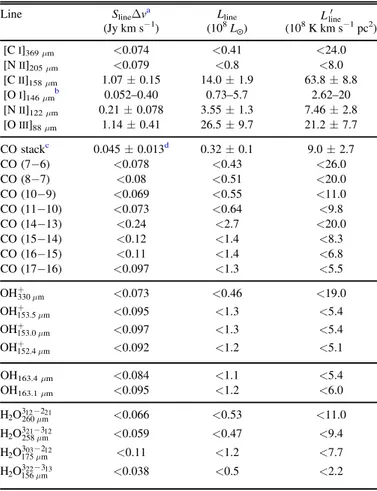
Fine Structure and Molecular Line Measurements in J1342+0928
Line SlineΔva Lline Lline¢
(Jy km s−1) (108 L☉) (108K km s−1pc2) [CI]369μm <0.074 <0.41 <24.0 [NII]205μm <0.079 <0.8 <8.0 [CII]158μm 1.07±0.15 14.0±1.9 63.8±8.8 [OI]146μmb 0.052–0.40 0.73–5.7 2.62–20 [NII]122μm 0.21±0.078 3.55±1.3 7.46±2.8 [OIII]88μm 1.14±0.41 26.5±9.7 21.2±7.7 CO stackc 0.045±0.013d 0.32±0.1 9.0±2.7 CO(7−6) <0.078 <0.43 <26.0 CO(8−7) <0.08 <0.51 <20.0 CO(10−9) <0.069 <0.55 <11.0 CO(11−10) <0.073 <0.64 <9.8 CO(14−13) <0.24 <2.7 <20.0 CO(15−14) <0.12 <1.4 <8.3 CO(16−15) <0.11 <1.4 <6.8 CO(17−16) <0.097 <1.3 <5.5 m + OH330 m <0.073 <0.46 <19.0 m + OH153.5 m <0.095 <1.3 <5.4 m + OH153.0 m <0.097 <1.3 <5.4 m + OH152.4 m <0.092 <1.2 <5.1 OH163.4μm <0.084 <1.1 <5.4 OH163.1μm <0.095 <1.2 <6.0 m -H O2 260 m312 221 <0.066 <0.53 <11.0 m -H O2 258 m321 312 <0.059 <0.47 <9.4 m -H O2 175 m 303 212 <0.11 <1.2 <7.7 m -H O2 156 m322 313 <0.038 <0.5 <2.2
Notes. Flux densities were measured inside a 2 6 diameter aperture, unless stated otherwise, and corrected for the residual. Upper limits correspond to 3σ of the local rms noise.
a
In all casesΔv=455km s-1, except for
m O I146 m
[ ] whereΔv=336km s-1
due to availability of fewer channels.
b
Given insufficient surface brightness sensitivity of the higher resolution map we report a 3σ upper limit on the aperture integrated emission, and a lower limit from the 3.9σ significant single beam measurement.
c
Stack of four CO lines in bands 3 and 4: CO(7−6), (8−7), (10−9), and (11 −10).
d
Peak surface brightness and rms is reported(it is consistent with aperture integration within the errors, but has a higher S/N).
Figure 3.Cutouts of J1342+0928 showing the emission line in the central panel. Left and right panels demonstrate the absence of the continuum emission due to its successful subtraction. Each panel containsflux integrated over a width of 455 km s−1(1.2×FWHM of the[C II]158 mm line), with the exception of[O I]146 mm where the central panel is 336 km s−1, due to its proximity to the sideband edge. Aperture used forflux integration is shown as the white dotted circle(diameter of 2 6). The synthesized beam is shown in the lower left corner of the middle panel. Full(dashed) contours represent the +(-) 2σ, 4σ and 8σ emission significance. The rms values in the middle panel are, from top to bottom: 35, 39, 85, 318, and 30 mJy beam-1. The cross marks the dust
continuum emission center in the high-resolution data(same as in Figure1). The bottom three panels show a stack of four CO lines in bands 3 and 4 (Jup=11, 10, 8, and 7).
extracted at the peak of the stacked emission.9Data in the higher frequency bands have higher noise or poorer resolution, and the expected CO brightness is lower for higher J transitions, therefore we do not include them in our CO stack(we stacked them separately, but no significant detection was recovered). For the sake of convenience, we will treat the four line stack as a tentative CO (9−8) detection, because this transition frequency corresponds to the mean frequency of the stacked lines. However, the effective frequency of the stacked emission is strongly dependent on the actual shape of the CO SED, which is presently unknown.
We stacked two water lines in band 4 (260 and 258 μm), resulting only in a 3σ upper limit on line flux density of 0.045Jy km s-1. The remaining two available water lines were observed at significantly different resolutions, and convolving all water lines to the same beam would result in a degraded signal quality.
3.3. Properties of the ISM
In the following sections we focus on specific lines and their ratios to derive various properties of the ISM in J1342+0928.
3.3.1. The FIR Line Deficit
An empirical observation showing a decrease in the
m
C II158 m
[ ] line-to-FIR continuum ratio with increasing dust temperature and IR luminosities is referred to as the line deficit (e.g., Malhotra et al.1997; Díaz-Santos et al.2013). The same
trend was observed in other fine structure lines, thanks to systematic studies with Herschel(e.g., Díaz-Santos et al.2017).
The ISM conditions leading to such results are still under investigation and several scenarios have been proposed. These include a change in the ionization parameter, various optical depth effects, or galaxy compactness (for details see, e.g., Graciá-Carpio et al. 2011; Herrera-Camus et al. 2018; Rybak et al.2019).
We report several fine structure line-to-FIR ratios of J1342 +0928 in Figure4, along with a recent study of local luminous infrared galaxies (LIRGs; LTIR=1010−11 L☉) performed by
Díaz-Santos et al. (2017). Measurements obtained on our
z=7.5 quasar host galaxy are consistent within the scatter with trends observed in the local LIRGs.
3.3.2. Photodissociation Regions(PDRs)
The type of radiationfield the ISM is subjected to divides its physical and chemical processes into two distinct regimes: the PDRs (also photon dominated regions) and the X-ray dissociation regions (XDRs; also X-ray dominated regions). The former implies the main source of energy are far-ultraviolet photons with energies between 6 and 13.6eV originating in O and B stars, and is therefore tied with star formation processes (see, e.g., Tielens & Hollenbach1985). In the latter regime, the
gas is illuminated by hard X-ray radiation (energies above 1 keV), which penetrates much deeper into the molecular clouds before being absorbed(see, e.g., Maloney et al. 1996).
Such hard radiation can originate in supermassive black hole accretion episodes and is therefore indicative of significant
AGN activity. In order to tie our observations to the underlying physical
properties, we make use of the PDR and XDR grid models developed by Meijerink & Spaans(2005) and Meijerink et al.
(2007). These models include various heating and cooling
Figure 4. Ratio between various fine structure lines and the FIR (42.5− 122.5μm) luminosities as a function of estimated dust temperature demonstrat-ing the line deficit. Our J1342+0928 measurements are shown with a red point. The accompanying red shaded area encompasses the considered dust temperature range in the horizontal direction and theflux density measurement error in the vertical direction. The blue line shows thefit to the local trend in LIRGs, while the dotted lines outline its 1σ dispersion (only the upper bound is constrained for the[O III]88 mm case), as reported in Díaz-Santos et al. (2017).
Figure 5.Constraints on the radiationfield intensity (in units of the Habing flux, G0=1.6×10⁻³ erg cm−2s−1) and the density of the ISM in J1342
+0928 based on the PDR model grid from Meijerink et al. (2007). Colored lines correspond to contours in the parameter space defined by specific line luminosity ratios, namely[C II]158 mm CO 7( -6)>33(yellow),[C II]158 mm
- >
CO 8( 7) 27(blue), <3 [C II]158 mm [O I]146 mm <19(red hatched area), and[C II]158 mm [C I]369 mm >34(black).
9
We note that this value is consistent with the aperture integration within the errors, but has a higher S/N.
processes and chemical reactions that reproduce emission line luminosities as a function of physical parameters, such as the radiation field and density of the ISM. For the PDR calculations, we may consider only emission arising in the neutral medium. The[C II]158 mm can originate in the ionized
medium as well; however, we will show in Section 3.3.5that this fraction can be constrained to less than 25%. Since we can only obtain an upper limit, we do not correct for the emission fraction arising in ionized medium, and assume that the entire
m
C II158 m
[ ] emission is dominated by the PDR.
The line luminosity ratio[C II]158 mm [C I]369 mm is useful for
discerning between the two main regimes(PDR and XDR) as the ratio is expected to be below 6 in XDRs regardless of ISM density or the radiationfield (see Figure 6 in Venemans et al.
2017c). Although we do not detect the[C I]369 mm line, its upper
limit sets a lower limit on the line luminosity ratio >
m m
C II158 m C I369 m 34
[ ] [ ] , which rules out XDR as the
dominant regime in J1342+0928. We can therefore assume pure PDR models for the subsequent analysis. In PDRs, the ratio of [C II]158 mm and CO emission lines is strongly
dependent on the density, and we can use our limits listed in Table2 to define an area in the density versus radiation field parameter space, which J1342+0928 occupies. As shown in Figure 5, PDR model parameters, which are derived from our limits, suggest densities of 5×104cm−3 and radiation field intensity of 103G
0, where G0 is the Habing flux
(G0=1.6×10⁻³ erg cm−2s−1). For comparison, similar
ISM studies performed in five different z>6 quasars (see Wang et al. 2016; Venemans et al. 2017a, and Yang et al.
2019) find densities higher than 105cm−3, and radiationfield intensities of the order of∼103G0. On the other hand, several
studies based on CO excitation ladders suggest densities in the range of 104-5cm−3 (see Weiß et al. 2007; Riechers et al.
2009).
3.3.3. Carbon Mass
The measured upper limit of the[C I]369 mm emission line can
provide constraints on the atomic carbon content of the galaxy. Following Weiß et al.(2003,2005) we can estimate the mass of
the neutral carbon as
= ´ - ¢ -m M M Q T e L 4.566 10 1 5 K km s pc , 8 T T C I 4 ex C I 1 2 2 ex 369 m ( ) ( ) [ ] [ ] whereQ T =1 +3e-T T +5e-T T ex 1 ex 2 ex
( ) is the partition
func-tion, excitation energies of two different carbon transitions are T1=23.6 K and T2=62.5 K, and the excitation temperature
is assumed to be Tex=30 K (see Walter et al.2011). Resulting
atomic carbon mass limit is M[C I]<5.3´106M. Walter et al.(2011) derived an atomic carbon to molecular hydrogen
abundance of X C I X H[ ] [ 2]=M[C I] (6MH2)=(8.43.5)´
-10 5 using a sample of z>2 submillimeter and quasar host galaxies. If we apply the same scaling relation to J1342+0928 we obtain MH2<1010M implying a gas-to-dust ratio upper
limit of<250.
For completeness, we mention here the ionized carbon mass of M[C II]=4.9´106M as reported by Venemans et al. (2017b), emitted from the outer layers of the PDR assuming
Tex=100 K (temperature range from 75 to 200 K would give a
20% difference on the estimated mass). 3.3.4. Gas Mass
In this section we constrain the total molecular gas mass of J1342+0928 employing a variety of methods. They are listed in Table 3 and explained below. The most common approach involves using the CO molecule as an H2 tracer. In order to
obtain the gas mass from the CO line emission, we must assume a CO-to-H2(light-to-mass) conversion factor αCO(see Bolatto
et al. 2013). The scaling is linear with line luminosity and
is defined as MH2[M☉]=aCOLCO 1 0¢ ( - )[K km s-1pc2]. We employ a value of aCO =0.8M☉(K km s-1pc2)-1(see Downes & Solomon 1998), which is often used. However, we note
that a broader range of aCO=0.3-2.5M☉(K km s-1pc2)-1 is recommended for ULIRGs(see Bolatto et al.2013). The αCO
factor is highly uncertain largely due to unknown average surface density of the giant molecular clouds and the kinetic temperature of the gas. To use this scaling relation, wefirst need to estimate the(unobserved) luminosity of the CO transmission of the rotational ground state.
One approach in estimating the CO(1−0) emission would be to use its empirical correlation with the FIR continuum,
¢ - - ~
L L L
log( FIR[ ] CO 1 0( )[K km s 1pc2]) 2 with a scatter of 0.5 dex, as shown in Figure 7 of Carilli & Walter(2013). This
correlation would imply LCO 1 0¢ ( - ) ~100´10 K km s8 -1pc2, and thus a high gas-to-dust mass ratio of∼230.
Table 3
The Total Gas Mass of J1342+0928 Estimated Using Different Proxies (see Section3.3.4for Details)
Proxy and Extrapolation Gas Mass Gas-to-dust (108M
) ratio
CO to FIR continuum correlation 80 230 CO(7−6) with J1148+5251 SLED <35 <100
CO stack with Class III SLED 11 30
m C II158 m
[ ] calibration 420 1200
Note.Conversion factor of aCO=0.8M☉(K km s-1pc2)-1is used for all CO measurements.
Figure 6.Constraints on the CO spectral line energy distribution of J1342 +0928 as a function of the rotational quantum number. The dotted black line shows the mean trends observed in local ULIRGs(see Rosenberg et al.2015), scaled to our stacked measurement(gray shaded area shows the scatter). The dashed orange line shows the CO SLED model of a z=6.4 quasar (Stefan et al.2015) scaled to our CO(7−6) upper limit.
We have a significant number of CO upper limits as well as a tentative stack detection, as shown in Figure6. If the CO(9−8) is thermalized it would implyLCO 1 0¢ ( - ) = ¢LCO 9 8( - ). A correc-tion to this simplified model involves usage of a CO spectral line energy distribution (SLED) of a high-redshift quasar. Stefan et al.(2015) employed large velocity gradients to model
the CO SLED of J114816.64+525150.3, a z=6.4 quasar, using four observed CO transitions up to Jup=7. This model
is also shown in Figure6, scaled to our CO(7−6) upper limit. The model extrapolation beyond Jup 8 is consistent with
our stacked measurement within 2σ and predicts ¢LCO 1 0( -) <
´
-44 10 K km s8 1pc2, M < ´ M
35 10
H2 8 , and a
gas-to-dust ratio of<100, based on our CO(7−6) upper limit. We can also consider the CO(SLEDs) of the local ULIRGs. In Figure 6 we show the Class III CO SLED, which has a turnover at higher J levels, as reported by Rosenberg et al. (2015), scaled to our stack measurement. If we employ the CO
SLED of ARP299, a merger induced starburst belonging to the abovementioned Class III group, the lineflux of the CO(1−0) transition is ∼50 times weaker than the CO(9−8) transition, which from Equation (7) implies ¢LCO 1 0( - ) ~1.5LCO 9 8¢ ( - ) =
´
-13.5 10 K km s8 1pc2, M = 113 ´10
H2 ( ) 8 M☉ and a
somewhat small gas-to-dust mass ratio of ∼30.
Zanella et al.(2018) suggests to use the[C II]158 mm emission
as a tracer of molecular gas mass via the conversion factor of
a
= ~
m
MH2 L[C II]158 m [C II] 30M L, with a standard
devia-tion of 0.2 dex, based on a sample of main-sequence galaxies at z∼2. These authors report that the calibration is largely independent of the phase gas metallicity and the starburst behavior of the galaxy. When applied to J1342+0928 we obtain molecular mass of MH2~4´1010M. This would
imply very large gas-to-dust ratios of ∼1200 and is not consistent with our nondetection of neutral carbon (see Section 3.3.3). Although large uncertainties are involved in
the estimates, our upper limits and the tentative stack detection, paired with different models of the CO SLEDs, do not favor such a large dust ratio. For comparison, standard gas-to-dust ratios observed in nearby galaxies are around∼100 (e.g., Sandstrom et al. 2013).
3.3.5. Ionized Gas
Due to different ionization energies of thefine structure lines (for C+, O+, N+, and O++they are 11.3, 13.6, 14.5, and 35 eV
respectively), and their critical densities,10 line ratios can further constrain the properties of the ISM, specifically the HII regions. The [N II]205 mm lines originate exclusively in the
ionized medium due to its ionization energy being higher than that of hydrogen (13.6 eV). The model provided by Oberst et al. (2006), see their Figure 2, which assumes an electron
impact excitation and electron temperature of 8000 K, allows us to use our measurement of[N II]122 mm [N II]205 mm >4.4to
set a lower limit on the electron density of ne>180 cm−3,
hence the N+emission is dominated by the HIIregions and not the diffuse ISM.
Carbon has a lower ionization energy than hydrogen allowing the [C II]158 mm emission line to arise in neutral and ionized
medium. Both transitions [C II]158 mm and [N II]205 mm have similar critical densities, 40 cm−3 and 44 cm−3, respectively, implying that their line luminosity ratio will depend solely on
their abundance ratio. This fact allows us to use their line ratio in order to disentangle the fraction of emission arising in different phases of the ISM. At the limit obtained above for the electron density (ne>180 cm−3), the expected value of the carbon to
nitrogen line ratio inside the ionized medium, according to Oberst et al. (2006), is 3 [C II]158 mm [N II]205 mm <4.3.
From this ratio, and our [N II]205 mm luminosity limit of
<0.8×10⁸ L
e, we can derive an upper limit on the m
C II158 m
[ ] emission arising from the ionized medium of < ´
m L
C II158 mion 3.4 108
[ ] . This accounts for less than 25%
of the entire14´108L
observed[C II]158 mm emission.
Following Ferkinhoff et al. (2011), assuming high density
and high temperature limit so that all nitrogen is singly ionized (valid around B2 to O8 stars), we can calculate the minimum H+mass required to produce the observed N+luminosity as
n c = + + m M L A h m H N , 9 g g N II 21 21 H t 122 m 2 ( ) ( ) ( ) [ ]
where parameters are statistical weight of the emission line g2=5, partition function gt=9, Einstein coefficient A21=
7.5×10⁻⁶s−1, relative abundance of nitrogen compared to hydrogen χ(N+)=9.3×10⁻⁵ (taken from Savage & Sem-bach1996), hydrogen atom mass mH, Planck constant h, and
the frequency of the 122μm line transition ν21. Inserting the
luminosity value ofL[N II]122mm=3.55´108L(from Table2)
yields Mmin(H+)=1.8´108M. When compared to the
molecular gas mass derived from the CO(7−6) upper limit we obtain a lower limit on the gas ionization percentage M(H+)/M(H2)>4%, while the estimate from the CO stack
measurement would yield an even greater value of∼16%. For comparison, the ionized gas fraction is observed to be less than <1% in nearby galaxies (see Figure 3 in Ferkinhoff et al.2011
based on Brauher et al. 2008 data), while larger ionization percentages point to the increased SFR surface density (~100 1000– M yr-1pc-2
).
A similar approach can be utilized for the O++ line, as described by Ferkinhoff et al. (2010). We can insert
into Equation(9) values valid for the[O III]88 mm line, namely
= ´
m
L[O III]88 m 26.5 108L, g2=3, gt=9, A21 =2.7´
-
-10 5s 1, χ(O++)=5.9×10⁻⁴ (from Savage & Sembach
1996), thus obtaining Mmin(H+)=0.7´108M. We do not expect all oxygen to be in the doubly ionized state (see Ferkinhoff et al.2010), so the minimum ionized gas we report
here is strictly a lower limit and it can easily be an order of magnitude higher.
Further investigation of ISM physical properties via emis-sion line ratios is available with the Cloudy spectral synthesis code(Ferland et al.2017). The model computes line strengths
on a grid of changing ISM conditions and we defer the details of the simulation and its setup to an upcoming paper by R. Decarli et al. 2019,(in preparation). Intensity of the radiation field can be estimated from the observed line ratio
=
m m
O III88 m N II122 m 7.5 4.0
[ ] [ ] . This is possible due to
the fact that both ions have similar critical densities, but different ionization energies. Assuming that stars with effective temperature of ∼40,000 K are responsible for the ionization radiation, the model predicts intensity of the radiationfield of
~
-U
log 2.5, where U is the ionization parameter defined as a ratio between the ionizing photon density and the total
10
De-excitation emission rates are equal to collision rates at the critical density.
hydrogen density (see, e.g., Draine 2011): U=n(hν>
13.6 eV)/nH. An equivalent way to write the ionization
parameter is U=Φ/(nH c), where Φ is the flux of the
hydrogen ionizing photons, and c is the speed of light. Assuming that the star formation is the main driver of observed atomic line emissions, we can usefindings reported in De Looze et al. (2014) to calculate the SFR of J1342+0928
using FIR fine structure lines. For high-redshift galaxies (z>0.5) these authors report the following calibration:
b a
= +
M L L
log SFR( ) log( line ), (10) where the parameters are α=1 and β=−6.89 for the
m
O III88 m
[ ] emission line, with a dispersion of 0.46 dex. This calibration yields SFR=340M yr-1
. Similarly, for
m
C II158 m
[ ] (α=1.18 and β=−8.52, dispersion 0.4 dex) we obtainSFR=180M yr-1
. Both of these values agree within the uncertainties with the SFR inferred from the dust continuum.
As is evident from Figure 3, the peak of the [O III]88 mm
emission is offset by 0 6 from the peak of the underlying continuum and peaks of other detected lines. Although this might be attributed to possible outflows (see, e.g., Bischetti et al.2017), the low S/N of our detection, and the fact that the
separation is less than one resolution element, does not allow for a robust interpretation. Theoretical studies performed by Katz et al.(2017,2019) predict that[O III]88 mm would be at an
offset from[C II]158 mm , because it arises from a medium with
higher temperatures and ionization parameter. They also predict that [N II]205 mm emission would be slightly more
extended compared to the[C II]158 mm emission. Deeper data,
preferably at higher resolution comparable to the [C II]158 mm
data, is required to investigate this potential offset further. Finally, we report oxygen-to-carbon line luminosity ratio of
=
m m
O III88 m C II158 m 1.9 0.7
[ ] [ ] , similar to other recent
high-redshift observations(see Hashimoto et al. 2018; Walter et al.2018).
3.3.6. Water
Water line emission originates in the warm dust (40–70 K) regions where densities are of the order of 105-6cm−3, and higher rotational CO lines(Jup>8) are also common (see Liu
et al. 2017). We do not detect any significant emission from
H2O, OH, and OH+species within 10 possible line candidates
that lie inside our observed frequency ranges. Water lines 312–221 at 260μm and 303–212 at 175μm show tentative
detections; however, the first one could be dominated by the neighboring CO(10−9) line, while the second one shows an excess in the spectrum, but a prominent negative peak at the required central frequency (see Appendix B). Our PDR
measurements(see Section3.3.2) point toward lower densities,
thus nondetection of water lines is consistent with ourfindings determined from CO nondetections.
3.3.7. Metallicity
Due to the high dust content and large SFRs, we expect that the ISM of J1342+0928 has already been enriched by the yields of supernovae. The metallicity of a galaxy is usually determined from optical line ratios, which are severely affected by dust extinction, and are not accessible to ground instruments for high-redshift objects. The FIR emission lines can provide an alternative method to measure metallicity, once it is properly
calibrated (see, e.g., Pereira-Santaella et al. 2017). The N++
and O++ ions are especially interesting for this study due to their similar ionization structure. We use the calibration reported by Rigopoulou et al. (2018), see their Figure 5, and
assume that the ionization parameter is logU= -2.5. From the [O III]88 mm [N II]122 mm =7.54 line ratio we derive
gas-phase metallicities in the HII region of Zgas=1.3-+0.10.3Z☉, where Z☉is the value for the solar neighborhood. A range of
U
log between −2 and −3 would yield metallicities of 0.7–2.0 Z☉, with line flux errors folded inside.
Multiple studies of high-redshift quasars performed using the optical spectra derive metallicities consistent with values observed in the solar neighborhood (see, e.g., Kurk et al.
2007; De Rosa et al. 2011; Mazzucchelli et al. 2017). These
measurements were obtained from the MgII / FeII line ratio measured in the broad line region, at spatial scales of1 kpc. On the other hand, our measurements, also pointing to solar like metallicities, are averaged across the entire galaxy host.
Rémy-Ruyer et al.(2014) have shown that the metallicity is
an important contributor to the observed gas-to-dust ratio. These authors report that the observed gas-to-dust ratio in their sample is around ∼100 for metallicities around solar, with a clear negative correlation between the two. Ourfindings of the rich metal content in the host galaxy of J1342+0928 are therefore in agreement with the low estimates on its gas-to-dust ratio derived from the CO limits(or the CO stack).
4. Conclusions
We have presented ALMA observations of the dust continuum and the ISM of the host galaxy J1342+0928, the most distant quasar known to date. The quasar was observed at z=7.54 when the universe was only 680 millions years old. With eight spectral setups positioned between 93.5 and 412 GHz, we constrain the Rayleigh–Jeans tail of the dust continuum and show that a modified blackbody with the canonical dust temperature of 47 K fits the data well. At the same time we narrow the dust spectral emissivity coefficient to β=1.85±0.3, derive the dust mass of Mdust=0.35×
108M☉and a high SFR of ~150M yr-1
.
With detections of atomic fine structure lines [C II]158 mm , m
N II205 m
[ ] , [O III]88 mm ; limits on [C I]369 mm , [N II]205 mm ,
m
O I146 m
[ ] ; and multiple CO lines (with a tentative stack detection) we derived the following main results. Observed line deficits in J1342+0928 are comparable to local ULIRGs. We do not see evidence of X-ray dominated regions, and photodissociation region-only model implies low gas densities (5×104cm−3) and strong radiation fields (103G
0). The
CO data hints at lower gas-to-dust ratios, less than 100. The[C II]158 mm emission originates predominantly inside the
neutral medium, and there is evidence of possible spatial offset between[C II]158 mm and[O III]88 mm emission. However, deeper
data is required to confirm and interpret this offset. A limit on the ratio of the two N++ emission lines imply high electron densities of ne>180 cm−3. We also find high percentages
(>4%, possibly ∼16%) of ionized to molecular hydrogen, indicating large SFR surface densities. We detect no water lines consistent with upper limits on CO lines and the derived density of the medium. Finally, we estimate that the metallicities are consistent with solar values, supporting the view of J1342+0928 as a galaxy extremely rich in dust and metals, despite the early epoch it is located in.
In this study of the ISM of a galaxy in the epoch of reionization, we demonstrate the wide range of investigations that are possible with ALMA observations of FIR emission lines. We have shown that such an analysis benefits greatly from observations of multiple lines arising in different states of the ISM. The coming years will provide more high-redshift candidates, and ALMA follow-ups targeting several FIR emission lines in these objects will lead to a deeper understanding of the ISM at the epoch of reionization.
We thank Dominik Riechers for helpful discussions and suggestions. Ml.N., F.W., B.V., and Ma.N. acknowledge support from the ERC Advanced Grant 740246 (Cosmic Gas). This paper makes use of the following ALMA data: ADS/JAO.ALMA#2017.1.00396.S. ALMA is a partnership of ESO(representing its member states), NSF (USA) and NINS (Japan), together with NRC (Canada), NSC and ASIAA (Taiwan), and KASI (Republic of Korea), in cooperation with the Republic of Chile. The Joint ALMA Observatory is operated by ESO, AUI/NRAO, and NAOJ. This research made use of Astropy,11a community-developed core Python package for Astronomy (Astropy Collaboration et al. 2013; Price-Whelan et al.2018), and Matplotlib (Hunter 2007).
Appendix A
Measuring Resolved Emission in Interferometric Maps The difficulty of properly interpreting the area of the synthesized beam in interferometric maps can have a detrimental effect on the accuracy of the measured flux density, especially for significantly resolved emission. A Fourier transform of measured visibilities is called a dirty map, where each pixel has a unit of jansky per dirty beam. The integral under the entire dirty beam is zero, because an integral of a single sine wave is zero, and the dirty beam is just a sum of various sine waves. During the cleaning process, the dirty beam is deconvolved from the map and replaced with a Gaussian beam with a properly defined integral. The cleaning process progresses down to some chosen threshold, and the final cleaned interferometric map is then a combination of the residual given in original units of jansky per dirty beam, and a cleaned component in units of jansky per clean beam (chosen to be a Gaussian). The end result is that units in the map are ill defined, and if the observed source is spread over multiple beams, the cumulative effect can be significant.
Several choices are available to tackle this problem. Thefirst one is to model the source using visibilities directly, without invoking the Fourier transform and going into the image plane. This works well for objects exhibiting some sort of symmetry, but is less useful for morphologically complex systems such as mergers, where a lot of details are hidden in the data coming from high-resolution/longer baselines. The second choice is to
clean very deep, which comes at a cost of treating every noise peak(both positive and negative) as emission. The third choice, which we employ in this paper, involves estimating the proper area of the dirty beam in the region of interest, as the dirty beam area is zero when integrated across all space, but is different from zero in a smaller region. This method is called the residual scaling and is outlined in Appendix A.2 of Jorsater & van Moorsel(1995), see also Walter & Brinks (1999) and
Walter et al.(2008). We summarize it here briefly.
We can consider the true flux G of a source as a sum of cleanedflux C in proper jansky per beam units, and the residual R, which has to be scaled to proper units in order to make the sum viable: G=C+ò R. The parameter ò corresponds to the clean beam to dirty beam area ratio. If the same map is cleaned down to two different thresholds, we have G=C1+ò
R1=C2+ò R2, because the true flux must be recovered
independent of the cleaning threshold. We can also choose not to clean, in which case C2=0 and R2is the dirty map. Solving
equations in this scenario yieldsò=C1/(R2−R1) and G=ò
R2. These calculations are performed within some aperture, and
use the dirty map R2, the clean flux map C1and the residual
map R1 to measure the flux density G. A drawback of the
residual scaling method arises in situations when R1≈R2, or
when there is not enough clean flux C1, and the solution
becomes numerically unstable.
In Figure 7 we demonstrate this method on our high-resolution (∼0 2) observations of J1342+0928 at 231.5 GHz and the[C II]158 mm line. The map was cleaned down to 2σ in a
2″ radius circle centered at the source. The flux density measured inside an aperture of r=1 3 from the usual map (clean components added on top of the residual) is 25% and 35% larger than the corrected one for the continuum and the line, respectively. The effect is more pronounced in sources with more extended emission and lower surface brightness, where a lot of flux remains in the residual. The numerical instability is evident in the continuum measurements at radii above 2″, as both the dirty map and the residual map measurements approach the same value.
In Figure8we show the residual scaling corrected aperture fluxes for different continuum bands and atomic fine structure lines. Here we motivate the aperture radius with a diameter of 2 6(radius of 1 3). The[C II]158 mm emission is detected at the
highest S/N and is the most extended, the flux density reaches a plateau at r=1 3. The chosen aperture size recovers the flux density measured at the plateau within the error bars in all of the maps. We therefore opt for the same aperture in all measurements for the sake of consistent interpretation of probed spatial scales of line ratios, despite observations being at different resolutions.
11
Appendix B
Spectra and Nondetections of J1342+0928
In order to properly constrain the width of a spectral line, at least 6σ is required in the central channel, so that the FWHM can be computed at a 3σ significance. All of our lines, except
m
C II158 m
[ ] , have less than 5σ in the moment zero map integrated over 455km s-1, and therefore have insufficient S/N
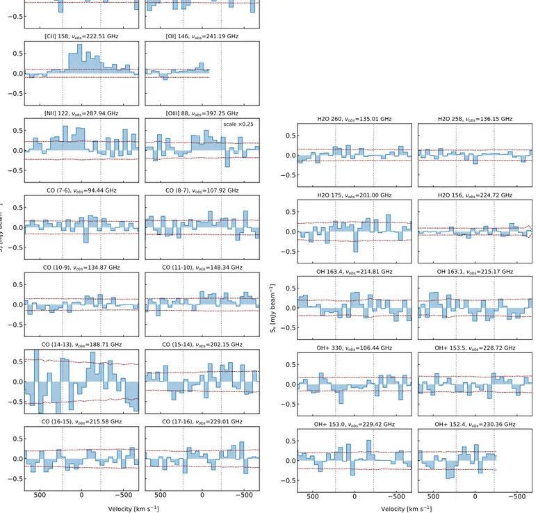
tofit a line profile in a meaningful way. However, since this work is a multiline spectral survey of an object, we show spectra of all considered lines in Figure 9 for completeness. The main goal of these spectra is to demonstrate the excess emission in individual channels. To maximize the S/N they are extracted from a single pixel.
Also for completeness, we show integrated moment zero maps of our emission line nondetections in Figures10and11. Figure 7.Apertureflux density of J1342+0928 observed with high resolution measured in various interferometric maps. Cleaning was performed down to 2σ in a 2″ radius circle. The clean beam size is used to convert from jansky per beam into jansky for all measurements. The green line representsflux density measured in the usual cleaned interferometric map. The red line demonstrates the effect of residual scaling correction. Left:continuum measurement at 231.5 GHz. Right:moment zero measurement of[C II]158 mm integrated over 455km s-1.
Figure 8.Flux density integrated inside an aperture as a function of its radius corrected with residual scaling. Left:continuum bands (see Table1). Right:atomic fine structure lines. The vertical line shows the aperture used throughout the paper.
Figure 9.Single pixel spectra of atomicfine structure lines and CO lines (left two columns) and H2O, OH, and OH+(right two columns) of J1342+0928, extracted
from the continuum subtracted cubes at the coordinate of the high resolution 231.5 GHz continuum peak. The red lines show the rms measured inside each, approximately 50 km s−1wide, channel. Vertical dashed lines encompass the 455 km s−1width used to measure the lineflux (see the text for details). Zero velocity corresponds to the redshifted line emission frequency(z=7.5413).
Figure 10.Nondetected atomicfine structure lines and CO lines in J1342+0928. Full (dashed) contours represent the +(-) 2σ, 4σ emission significance. The cross marks the dust continuum emission center in the high-resolution data(same as in Figure3).
ORCID iDs
Mladen Novak https://orcid.org/0000-0001-8695-825X
Eduardo Bañados https://orcid.org/0000-0002-2931-7824
Roberto Decarli https://orcid.org/0000-0002-2662-8803
Fabian Walter https://orcid.org/0000-0003-4793-7880
Bram Venemans https://orcid.org/0000-0001-9024-8322
Marcel Neeleman https://orcid.org/0000-0002-9838-8191
Emanuele Paolo Farina https://orcid.org/0000-0002-6822-2254
Chiara Mazzucchelli https://orcid.org/0000-0002-5941-5214
Chris Carilli https://orcid.org/0000-0001-6647-3861
Xiaohui Fan https://orcid.org/0000-0003-3310-0131
Hans–Walter Rix https://orcid.org/0000-0003-4996-9069
Feige Wang https://orcid.org/0000-0002-7633-431X
References
Astropy Collaboration, Robitaille, T. P., Tollerud, E. J., et al. 2013, A&A, 558, A33
Bañados, E., Novak, M., Neeleman, M., et al. 2019, ApJL, submitted
Bañados, E., Venemans, B. P., Decarli, R., et al. 2016,ApJS,227, 11 Bañados, E., Venemans, B. P., Mazzucchelli, C., et al. 2018,Natur,553, 473 Becker, G. D., Bolton, J. S., & Lidz, A. 2015,PASA,32, e045
Beelen, A., Cox, P., Benford, D. J., et al. 2006,ApJ,642, 694 Bischetti, M., Piconcelli, E., Vietri, G., et al. 2017,A&A,598, A122 Bolatto, A. D., Wolfire, M., & Leroy, A. K. 2013,ARA&A,51, 207 Brauher, J. R., Dale, D. A., & Helou, G. 2008,ApJS,178, 280 Carilli, C. L., & Walter, F. 2013,ARA&A,51, 105
Carniani, S., Gallerani, S., Vallini, L., et al. 2019, arXiv:1902.01413 Carniani, S., Maiolino, R., Pallottini, A., et al. 2017,A&A,605, A42 Chabrier, G. 2003,PASP,115, 763
da Cunha, E., Groves, B., Walter, F., et al. 2013,ApJ,766, 13 Daddi, E., Dannerbauer, H., Liu, D., et al. 2015,A&A,577, A46 De Looze, I., Cormier, D., Lebouteiller, V., et al. 2014,A&A,568, A62 De Rosa, G., Decarli, R., Walter, F., et al. 2011,ApJ,739, 56 De Rosa, G., Venemans, B. P., Decarli, R., et al. 2014,ApJ,790, 145 Decarli, R., Walter, F., Venemans, B. P., et al. 2018,ApJ,854, 97 Díaz-Santos, T., Armus, L., Charmandaris, V., et al. 2013,ApJ,774, 68 Díaz-Santos, T., Armus, L., Charmandaris, V., et al. 2017,ApJ,846, 32 Downes, D., & Solomon, P. M. 1998,ApJ,507, 615
Draine, B. T. 2011,ApJ,732, 100
Dunne, L., Eales, S. A., & Edmunds, M. G. 2003,MNRAS,341, 589 Fan, X., Strauss, M. A., Becker, R. H., et al. 2006,AJ,132, 117
Figure 11.Nondetected H2O, OH, and OH+emission lines in J1342+0928. Full (dashed) contours represent the +(-) 2σ and 4σ emission significance. The cross
Ferkinhoff, C., Brisbin, D., Nikola, T., et al. 2011,ApJL,740, L29 Ferkinhoff, C., Hailey-Dunsheath, S., Nikola, T., et al. 2010,ApJL,714, L147 Ferland, G. J., Chatzikos, M., Guzmán, F., et al. 2017, RMxAA,53, 385 Fischer, J., Sturm, E., González-Alfonso, E., et al. 2010,A&A,518, L41 Gallerani, S., Ferrara, A., Neri, R., & Maiolino, R. 2014,MNRAS,445, 2848 González-Alfonso, E., Fischer, J., Bruderer, S., et al. 2013,A&A,550, A25 Graciá-Carpio, J., Sturm, E., Hailey-Dunsheath, S., et al. 2011,ApJL,728, L7 Hashimoto, T., Inoue, A. K., Mawatari, K., et al. 2019,PASJ,70, psz049 Hashimoto, T., Inoue, A. K., Tamura, Y., et al. 2018, arXiv:1811.00030 Herrera-Camus, R., Bolatto, A., Smith, J. D., et al. 2016,ApJ,826, 175 Herrera-Camus, R., Sturm, E., Graciá-Carpio, J., et al. 2018,ApJ,861, 95 Hunter, J. D. 2007,CSE,9, 90
Jiang, L., McGreer, I. D., Fan, X., et al. 2016,ApJ,833, 222 Jorsater, S., & van Moorsel, G. A. 1995,AJ,110, 2037
Katz, H., Galligan, T. P., Kimm, T., et al. 2019,MNRAS,487, 5902 Katz, H., Kimm, T., Sijacki, D., & Haehnelt, M. G. 2017,MNRAS,468, 4831 Kennicutt, R. C., & Evans, N. J. 2012,ARA&A,50, 531
Kennicutt, R. C. J. 1998,ARA&A,36, 189
Kurk, J. D., Walter, F., Fan, X., et al. 2007,ApJ,669, 32 Liu, L., Weiß, A., Perez-Beaupuits, J. P., et al. 2017,ApJ,846, 5 Malhotra, S., Helou, G., Stacey, G., et al. 1997,ApJL,491, L27
Maloney, P. R., Hollenbach, D. J., & Tielens, A. G. G. M. 1996,ApJ,466, 561 Marrone, D. P., Spilker, J. S., Hayward, C. C., et al. 2018,Natur,553, 51 Matsuoka, Y., Strauss, M. A., Kashikawa, N., et al. 2018,ApJ,869, 150 Mazzucchelli, C., Bañados, E., Venemans, B. P., et al. 2017,ApJ,849, 91 McMullin, J. P., Waters, B., Schiebel, D., Young, W., & Golap, K. 2007, adass
XVI, 376 ed. R. A. Shaw, F. Hill, & D. J. Bell, 127 Meijerink, R., & Spaans, M. 2005,A&A,436, 397
Meijerink, R., Spaans, M., & Israel, F. P. 2007,A&A,461, 793 Oberst, T. E., Parshley, S. C., Stacey, G. J., et al. 2006,ApJL,652, L125 Pereira-Santaella, M., Rigopoulou, D., Farrah, D., Lebouteiller, V., & Li, J.
2017,MNRAS,470, 1218
Price-Whelan, A. M., Sipőcz, B. M., Günther, H. M., et al. 2018,AJ,156, 123 Rémy-Ruyer, A., Madden, S. C., Galliano, F., et al. 2014,A&A,563, A31
Riechers, D. A., Bradford, C. M., Clements, D. L., et al. 2013,Natur,496, 329 Riechers, D. A., Walter, F., Bertoldi, F., et al. 2009,ApJ,703, 1338 Rigopoulou, D., Pereira-Santaella, M., Magdis, G. E., et al. 2018,MNRAS,
473, 20
Rosenberg, M. J. F., van der Werf, P. P., Aalto, S., et al. 2015,ApJ,801, 72 Rybak, M., Calistro Rivera, G., Hodge, J. A., et al. 2019,ApJ,876, 112 Sandstrom, K. M., Leroy, A. K., Walter, F., et al. 2013,ApJ,777, 5 Savage, B. D., & Sembach, K. R. 1996,ARA&A,34, 279
Sijacki, D., Vogelsberger, M., Genel, S., et al. 2015,MNRAS,452, 575 Solomon, P. M., Downes, D., Radford, S. J. E., & Barrett, J. W. 1997,ApJ,
478, 144
Stefan, I. I., Carilli, C. L., Wagg, J., et al. 2015,MNRAS,451, 1713 Tadaki, K.-I., Iono, D., Hatsukade, B., et al. 2019,ApJ,876, 1 Tielens, A. G. G. M., & Hollenbach, D. 1985,ApJ,291, 722 van der Vlugt, D., & Costa, T. 2019, arXiv:1903.04544
van der Werf, P. P., Berciano Alba, A., Spaans, M., et al. 2011,ApJL,741, L38
Venemans, B. P., Walter, F., Decarli, R., et al. 2017a,ApJ,845, 154 Venemans, B. P., Walter, F., Decarli, R., et al. 2017b,ApJL,851, L8 Venemans, B. P., Walter, F., Decarli, R., et al. 2017c,ApJ,837, 146 Volonteri, M. 2012,Sci,337, 544
Walter, F., & Brinks, E. 1999,AJ,118, 273
Walter, F., Brinks, E., de Blok, W. J. G., et al. 2008,AJ,136, 2563 Walter, F., Riechers, D., Novak, M., et al. 2018,ApJL,869, L22
Walter, F., Weiß, A., Downes, D., Decarli, R., & Henkel, C. 2011, ApJ, 730, 18
Wang, R., Wagg, J., Carilli, C. L., et al. 2013,ApJ,773, 44 Wang, R., Wu, X.-B., Neri, R., et al. 2016,ApJ,830, 53
Weiß, A., Downes, D., Henkel, C., & Walter, F. 2005,A&A,429, L25 Weiß, A., Downes, D., Neri, R., et al. 2007,A&A,467, 955
Weiß, A., Henkel, C., Downes, D., & Walter, F. 2003,A&A,409, L41 Willott, C. J., Bergeron, J., & Omont, A. 2015,ApJ,801, 123 Yang, J., Venemans, B., Wang, F., et al. 2019, arXiv:1907.00385 Zanella, A., Daddi, E., Magdis, G., et al. 2018,MNRAS,481, 1976