The 2015-2016 Outburst of the Classical EXor V1118 Ori

2017

Publication Year

2021-02-22T11:28:01Z

Acceptance in OA@INAF

The 2015-2016 Outburst of the Classical EXor V1118 Ori

Title

GIANNINI, Teresa; ANTONIUCCI, Simone; LORENZETTI, Dario; MUNARI, Ulisse;

LI CAUSI, Gianluca; et al.

Authors

10.3847/1538-4357/aa6b56

DOI

http://hdl.handle.net/20.500.12386/30500

Handle

THE ASTROPHYSICAL JOURNAL

Journal

839

The 2015

–2016 Outburst of the Classical EXor V1118 Ori

T. Giannini1, S. Antoniucci1, D. Lorenzetti1, U. Munari2, G. Li Causi1,3, C. F. Manara4, B. Nisini1, A. A. Arkharov5, S. Dallaporta6, A. Di Paola1, A. Giunta1, A. Harutyunyan7, S. A. Klimanov5, A. Marchetti8, G. L. Righetti6, A. Rossi9, F. Strafella10, and V. Testa1

1

INAF—Osservatorio Astronomico di Roma, via Frascati 33, I-00078, Monte Porzio Catone, Italy;teresa.giannini@oa-roma.inaf.it

2_{INAF—Osservatorio Astronomico di Padova, via dell’ Osservatorio 8, I-36012, Asiago (VI), Italy} 3

INAF—Istituto di Astrofisica e Planetologia Spaziali, via Fosso del Cavaliere 100, I-00133, Roma, Italy

4_{Scientific Support Office, Directorate of Science, European Space Research and Technology Centre (ESA/ESTEC),}

Keplerlaan 1, 2201, AZ Noordwijk, The Netherlands

5

Central Astronomical Observatory of Pulkovo, Pulkovskoe shosse 65, 196140, St.Petersburg, Russia

6

ANS Collaboration, Astronomical Observatory, I-36012, Asiago(VI), Italy

7

Fundación Galileo Galilei—INAF, Telescopio Nazionale Galileo, E-38700, Santa Cruz de la Palma, Tenerife, Spain

8

INAF—Osservatorio Astronomico di Brera, Via Brera 28, I-20122, Milano, Italy

9

INAF—Osservatorio Astronomico di Bologna, via Ranzani 1, I-40127, Bologna, Italy

10

Dipartimento di Matematica e Fisica, Universitá del Salento, I-73100 Lecce, Italy Received 2017 February 1; revised 2017 March 31; accepted 2017 March 31; published 2017 April 24

Abstract

After a quiescence period of about 10 years,the classical EXor source V1118 Ori has undergone an accretion

outburst in 2015September. The maximum brightness (DV4 mag) was reached in2015Decemberand was

maintained for several months. Since 2016September, the source is in a declining phase. Photometry and low/

high-resolution spectroscopy were obtained with MODS and LUCI2 at the Large Binocular Telescope, with the facilities at the Asiago 1.22 and 1.82 m telescopes, and with GIANO at the Telescopio Nazionale Galileo. The

spectra are dominated by emission lines of HIand neutral metallic species. From line and continuum analysis we

derive the mass accretion rate and its evolution during the outburst. Considering that extinction may vary between 1.5 and 2.9 mag, we obtain ˙Macc=0.3–2.0 10−8Myr−1in quiescence and ˙Macc=0.2–1.9 10−6Myr−1at the

outburst peak. TheBalmer decrementshape has been interpreted by means of line excitation models, finding that

from quiescence to outburst peak, the electron density has increased from ∼2 109cm−3 to∼4 1011cm−3. The

profiles of themetallic lines are symmetric and narrower than 100 km s−1, while HIand HeIlines show prominent wings extending up to±500 km s−1. The metallic lines likely originate at the base of the accretion columns, where

neutrals are efficiently shielded against the ionizing photons, while faster ionized gas is closer to the star.

Outflowing activity is testified by the detection of a variable P Cyg-like profile of the Hα and HeI1.08μm lines. Key words: accretion, accretion disks – infrared: stars – stars: formation – stars: individual (V1118 Ori) – stars:

pre-main sequence– stars: variables: T Tauri, Herbig Ae/Be

1. Introduction

EXors are pre-main sequence objects showing eruptive

variability that iscaused by intermittent events of

magneto-spheric accretion(Shu et al.1994). Because of its relevance in the overall star formation process, the unsteady mass accretion phenomenon is a theme that has been largely investigated in the past decade, and a comprehensive review of the

phenomen-ological aspects hasrecently beengiven by Audard et al.

(2014). What is observed is essentiallya sequence

ofshort-duration outbursts (typically months) occurring at different

timescales(years) and showing different amplitudes. EXors are

believed to share the same triggering mechanism asFUors

objects (Hartmann & Kenyon 1985), but they present

substantial differences such as shorter and more frequent outbursts, spectra dominated by emission lines instead of absorption lines, and lower values of the mass accretion rate. Since a detailed model of the disk structure and its evolution

does not yetexistfor EXor stars, their phenomenology has so

farbeeninterpreted by adoptingthe theoretical approaches that

have beendeveloped forstudyingFUor events (e.g., Zhu

et al. 2009). In this framework, D’Angelo & Spruit (2010) provided quantitative predictions for the episodic accretion of piled-up material at the inner edge of the disk.

Although the details of the mechanism responsible for the onset of EXor accretion outbursts are not known, two main

scenarios have been proposed, which involve(1) disk

instabil-ity, and(2) perturbation of the disk by an external body. The

first group of models considers gravitational, thermal, or magnetospheric instabilities. While gravitational instabilities (e.g., Adams & Lin 1993) do not predict the observed short

timescale of the photometric fluctuation, thermal instabilities

(Bell & Lin 1994) offer a more acceptable explanation. They occur when the disk temperature reaches a value of about

5000 K and the opacity becomes a strong function of any(even

very small) temperature fluctuation. Thermal models, however,

present some difficulties and limitations that aremainly related to the unrealistic constraints on the disk viscosity. Alterna-tively, outbursts might be indirectly triggered by stellar dynamo cyclesviaradial diffusion of the magnetic field across the disk

(Armitage 2016). Inthe second group of models, several

relevant mechanisms have been considered, such asa massive

planet that opens up a gap in the disk(Lodato & Clarke2004) thatis thenable to trigger thermal instabilities at the gap itself.

Alternatively, accretion bursts can be causedby an external

trigger such as a close encounter in a binary system(Bonnell & Bastien1992; Reipurth & Aspin2004).

The lack of specific models is also related to adescription of the onset phase that is not detailed enough. Hence a monitoring that continuously follows the pre-outburst and the outburst evolution is fundamental in order to provide the variations of

both the photometric (lightcurve, colors) and spectroscopic

properties (line excitation, ionization, dynamics). Remarkable

efforts in this sense have been made by Sicilia-Aguilar et al. (2012) and Hillenbrand et al. (2013), who give details of the last outburst of EX Lup, the prototype of the class, and the

more embedded V2492 Cyg. Another classicalfrequently

monitored EXor is V1118 Ori (aJ 2000.0 =05 34 44. 745h m  , dJ 2000.0= -  ¢ 05 33 42. 18): its flare-upsin the past 40 years have been photometrically documented in the optical bands (e.g., Parsamian et al. 1993, 1996, 2002; Garcia Garcia &

Parsamian 2000, 2008; Audard et al. 2005, 2010;

Jurdana-Šepić et al. 2017a), andin particular, we followed different

phases of activity during the past 10 years (Lorenzetti

et al. 2006, 2009, 2015a, hereafter Paper I), while Audard

et al. have performed a detailed photometric monitoring of the

2005 outburst thatspanneda wide interval of frequencies

fromnear- and mid-IRtoX-rays. In the framework of our

monitoring program EXORCISM(EXOR optiCal and Infrared

Systematic Monitoring, Antoniucci et al. 2014), we have

discovered a new outburst of V1118 Ori in September 2015(Lorenzetti et al. 2015b; Giannini et al.2016, hereafter PaperII).

In this work we present the optical and near-IR follow-up observations of this last outburst. Our aim is to provide a global picture of all the outburst phases (rising, peak, and declining) from an observational point of view. Photometric and

spectroscopic observations are presented in Section 2and

areanalyzed and discussed in Section 3. Our concluding

remarks are given in Section4.

2. Data

2.1. Literature and Archival Photometry

To have a complete view of the photometric activity of V1118 Ori, we have searched the literature and public archives to construct its multiwavelength historical lightcurve. This is

depicted in Figure1(where our new data are alsoshown) and

commented in Section3.1.1. We collected data since 1959 for

the bands UBVRIJHK (references are in the figure caption),

WISE/1–3 (at 3.4/4.6/12 μm), Spitzer/IRAC (3.6/4.5/5.8/

8.0μm), and Spitzer/MIPS (24 μm). Spitzer data are published

in Audard et al. (2010), while Wide-field Infrared Survey

Explorer (WISE) data are reported here for the first time

(Section 2.2.3). For completeness, we alsoaccountfor a few

data before the 1960s, which indicate a remarkable level of

activity (mpg ~14.0) in 1939, 1956, and 1961 (Paul

et al.1995).

2.2. New Photometry

The new photometry covers the period 2015 December–

2016 December. Together with the photometryreported in

Figure 1.Historical lightcurve of V1118 Ori. Optical/near-IR and mid-IR magnitudes are represented with filled and open circles, respectively. Magnitudes in differentfilters are depicted with different colors, as indicated UBVRIJHK photometry was taken fromAudard et al. (2005,2010), Garcia Garcia et al. (1995,2006),

Garcia Garcia & Parsamian(2000,2008), Gasparian & Ohanian (1989), Jurdana-Šepić et al. (2017b), Hayakawa et al. (1998), Hillenbrand (1997), Parsamian &

Gasparian(1987), Parsamian et al. (1993,1996,2002), PapersI,II, Verdenet et al. (1990), andWilliams et al. (2005). We have also retrieved data from the

catalogsAAVSO (BVRI), 2MASS (JHK ), DENIS (IJK ), WISE (3.4/4.6/12 μm, W1–W3), Spitzer/IRAC (3.6/4.5/5.8/8.0 μm, I1–I4), and Spitzer/MIPS (24 μm, M1).

PapersI,IIit follows the evolution of the 2015–2016 outburst

fromquiescence to the post-outburst phases. In Figure 2 we

show the lightcurve from 2015 January–2016 December,

where we have empirically identified fivephasesto which we

refer in the analysis: (1) quiescence: up to 2015 March; (2)

rising: 2015 October; (3) peak: 2015 November–2016 April;

(4) declining: 2016 September; and(5) post-outburst: since 2016 December.

2.2.1. Optical Photometry

BVR IC Coptical photometry of V1118 Ori has been obtained

with the Asiago Novae and Symbiotic stars(ANS)

Collabora-tion telescopes 36 and 157, 0.3 m f/10 instruments located in

Cembra and Granarolo (Italy). Technical details and

opera-tional procedures of the ANS Collaboration network of

telescopes are presented by Munari et al. (2012), while

analyses of the photometric performances and multi-epoch

measurements of the actual transmission profiles for all the

photometric filter sets are discussed by Munari & Moretti

(2012). The same local photometric sequence was used at both

telescopes in all observing epochs, ensuring a high consistency of the data. The sequence was calibrated from APASS survey data (Henden et al.2012; Henden & Munari 2014) using the

SLOAN-Landolt transformation equations calibrated in Munari

(2012) and Munari et al. (2014a, 2014b). Reduction was

achieved by using standard procedures for bad-pixel cleaning,

bias and dark removal, andflat fielding. All measurements were

carried out with aperture photometry, the long focal length of

the telescopes, and withoutnearby contaminating stars, which

meant that we werenot requiredto revert to point-spread

funtion(PSF-) fitting.

The BVR IC C photometry of V1118 Ori is given in Table1

and shown in the top panel of Figure 2. The source has

remained bright(with daily variations ofup to 0.4 mag in V )

throughoutthe monitoring period until 2016 April, when

observations had to be momentarily halted for solar conjunc-tion. They restarted in 2016 August, and at that time, the visual

magnitudedropped byabout 1 mag. Since 2016 August,

V1118 Ori has continued to rapidly fadeto V»16.5 mag,

even ifit has not reachedthe magnitude (V≈17–18 mag)

typical of its quiescent state at present.

2.2.2. Near-infrared Photometry

JHK aperture photometry was achieved with the 1.1 m

AZT-24 telescope at Campo Imperatore (L’Aquila, Italy)

with the SWIRCAM camera (D’Alessio et al. 2000). Data

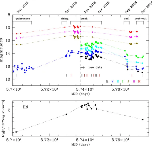
Figure 2.Top panel: optical and near-IR lightcurve in the period 2015 January–2016 December. Colors indicate the same bands as in Figure1. Data taken after the date marked with a dashed vertical line are reported in this paper for thefirst time, while those before that date are taken from the literature. These are shown to have a global view of the 2015–2016 outburst. Different temporal phases are labeled: (1) quiescence: up to 2015 March; (2) rising: 2015 October; (3) peak: 2015 November– 2016 April;(4) declining: 2016 September; and(5) post-outburst: since 2016 December. Vertical black andred segments indicate the dates when optical andnear-IR spectra were taken. Bottom panel:flux of the Hβ line as a function of time.

reduction was performed by using standard procedures for

bad-pixel cleaning,flat fielding, and sky subtraction.

Calibra-tion was achieved on the basis of 2MASS photometry of

severalbright starsin the field. We present in Table 2 and

Figure 2 (top panel) the data obtained between 2015

December and 2016 November, which follow those provided in PapersIandII. The peak of the infrared activityoccurred between 2015 December and 2016 February. No data are available between 2016 March and September; after this period, the source has faded and reached the quiescence value in all the near-IR bands(see PaperI).

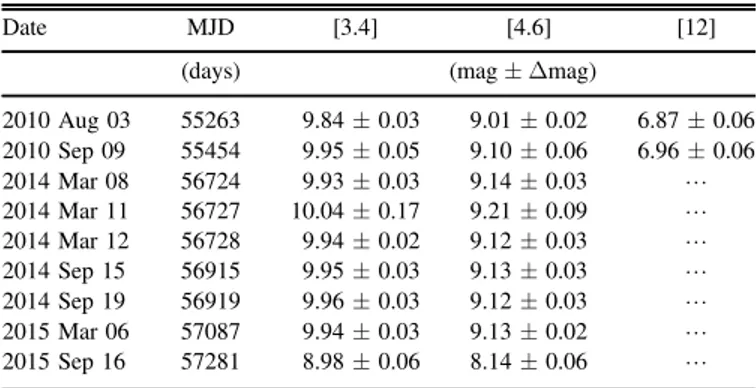
2.2.3. WISE Photometry

V1118 Ori was also observed in its quiescent phase byWISE

(Wright et al.2010)during both the cryogenic (2009 December–

2010 August) and the three-band (2010 August–September)

surveys(see Table3). Average values of the WISE magnitudes

are [3.4]=9.9, [4.6]=9.0, and[12]=6.9, [22] > 3.4 mag.

More recent observations have been collected in the first two

bands during the ongoing Neowise-R survey. Measurements

taken on 2015 September 16 are [3.4]=8.9 and [4.6]=8.1,

with a brightness increase of≈1 mag in both bands with respect to the quiescence values.

2.3. Spectroscopy

V1118 Ori has been spectroscopically observed in low- and

high-resolution configurations at optical and near-IR

wave-lengths. A journal of the spectroscopic observations is given in Table4.

2.3.1. Optical Spectroscopy

Four optical low-resolution spectra have been collected on

2016 January 12, 26, and 31 and 2016 December 4with the

8.4 m Large Binocular Telescope(LBT) using the Multi-Object

Double Spectrograph (MODS—Pogge et al. 2010). All

observations have been taken with the dual grating mode(blue

+ red channels) and integrated 1500 s in the spectral range

3200–9500Å using a 0 8 slit ( ~R 1500). Data reduction was

Table 1 Optical Photometry Date MJD B V Rc Ic Tel. (days) (mag) 2016 Jan 06 57393.412 14.59 13.83 13.24 12.51 036 2016 Jan 13 57400.420 14.59 13.92 13.28 12.56 036 2016 Jan 14 57401.371 14.66 14.08 13.39 12.68 157 2016 Jan 16 57403.251 14.51 13.89 13.18 12.53 157 2016 Jan 17 57404.352 14.79 14.01 13.38 12.63 036 2016 Jan 20 57407.357 14.81 14.14 13.51 12.76 036 2016 Jan 26 57413.230 14.43 13.75 13.09 12.41 157 2016 Jan 26 57413.245 14.51 13.78 13.18 12.43 036 2016 Feb 01 57419.427 L 14.08 13.48 12.74 036 2016 Feb 06 57424.234 14.96 14.28 13.52 12.83 157 2016 Feb 06 57424.253 14.89 14.26 13.56 12.82 036 2016 Feb 12 57430.236 14.89 14.32 13.63 12.95 157 2016 Feb 19 57437.242 14.97 14.49 13.86 13.09 157 2016 Feb 20 57438.243 14.84 14.17 13.40 12.74 157 2016 Feb 21 57439.296 14.53 13.72 13.06 12.47 036 2016 Feb 21 57439.312 14.26 13.74 13.17 12.49 157 2016 Feb 21 57439.362 L 13.71 L 12.46 036 2016 Feb 22 57440.259 14.59 14.09 13.20 12.55 157 2016 Feb 22 57440.364 14.45 13.75 12.97 12.42 036 2016 Feb 24 57442.249 14.46 13.85 13.14 12.48 157 2016 Mar 02 57449.244 14.72 13.98 13.36 12.63 157 2016 Mar 02 57449.319 14.59 14.00 13.38 12.61 036 2016 Mar 15 57462.257 14.18 13.53 12.84 12.17 157 2016 Mar 15 57462.281 14.23 13.58 12.88 12.19 036 2016 Mar 18 57465.256 14.28 13.56 12.93 12.26 157 2016 Mar 19 57466.258 14.38 13.72 13.01 12.29 157 2016 Mar 19 57466.316 14.43 13.67 13.00 12.30 036 2016 Mar 24 57471.301 14.55 13.79 L 12.41 036 2016 Mar 30 57477.284 14.42 13.75 13.08 12.39 157 2016 Apr 12 57490.279 14.58 13.80 13.06 12.36 157 2016 Apr 16 57494.285 14.65 13.84 13.14 12.42 157 2016 Aug 25 57625.622 L 14.50 L 13.59 036 2016 Sep 06 57637.619 15.97 15.64 14.94 14.16 157 2016 Sep 09 57640.637 16.51 16.10 15.28 14.31 157 2016 Oct 27 57688.675 L 15.99 L 14.35 036 2016 Oct 29 57690.455 16.42 16.34 15.36 14.45 157 2016 Nov 11 57699.466 16.81 16.54 15.41 14.64 157 2016 Nov 30 57723.435 16.97 16.41 15.52 14.64 157 2016 Dec 05 57728.473 L 16.28 L 14.43 036

Note.Typical errors are smallerthan 0.02 mag.

Table 2 Near-IR Photometry Date MJD J H K (days) (mag) 2015 Dec 18 57374.474 11.34 10.63 9.83 2016 Feb 02 57442.356 11.45 10.69 9.89 2016 Feb 24 57442.366 11.46 10.68 L 2016 Sep 21 57652.574 12.49 11.41 10.57 2016 Sep 23 57654.600 12.53 11.47 10.71 2016 Sep 25 57656.616 12.58 11.51 10.76 2016 Sep 27 57658.612 12.56 11.51 10.74 2016 Sep 28 57659.597 12.55 11.51 10.75 2016 Sep 30 57661.580 12.46 11.41 10.62 2016 Oct 01 57662.667 12.57 11.50 10.67 2016 Oct 29 57690.548 12.42 11.33 10.67 2016 Oct 31 57692.598 12.46 11.41 10.65 2016 Nov 02 57694.504 12.47 11.39 10.61

Note.Typical errors are smallerthan 0.03 mag.

Table 3 WISE Photometry

Date MJD [3.4] [4.6] [12]

(days) (mag ± Δmag)

2010 Aug 03 55263 9.84±0.03 9.01±0.02 6.87±0.06 2010 Sep 09 55454 9.95±0.05 9.10±0.06 6.96±0.06 2014 Mar 08 56724 9.93±0.03 9.14±0.03 L 2014 Mar 11 56727 10.04±0.17 9.21±0.09 L 2014 Mar 12 56728 9.94±0.02 9.12±0.03 L 2014 Sep 15 56915 9.95±0.03 9.13±0.03 L 2014 Sep 19 56919 9.96±0.03 9.12±0.03 L 2015 Mar 06 57087 9.94±0.03 9.13±0.02 L 2015 Sep 16 57281 8.98±0.06 8.14±0.06 L

performed at the Italian LBT Spectroscopic Reduction

Center11by means of scripts optimized for LBT data. Steps

of the data reduction of each two-dimensional spectral image

arecorrection for dark and bias, bad-pixel mapping,

flat-fielding, sky background subtraction, and extraction of one-dimensional spectrum by integrating the stellar trace along the spatial direction. Wavelength calibration was obtained from the

spectra of arc lamps, whileflux calibration was achieved using

the ANS Collaboration telescopes photometry, taken within one day from the spectroscopic observations.

Seven additionalspectra (3300–8050 Å) at R~2400 were

obtained with the 1.22 m telescope+B&C spectrograph operated in Asiago by the University of Padova. The slit has been keptfixed at a width of 2″and wasalways aligned with the parallactic angle for optimal absoluteflux calibration.

Finally, six high-resolution spectra in the range of 3600–7300Å were taken with the REOSC Echelle spectrograph mounted on the 1.82 m telescope operated in Asiago by the National Institute

of Astrophysics (INAF). The spectrograph covers the whole

wavelength interval in 32 orders without interorder gaps. The slit width was set to provide a resolving power of 20,000, and—as for the 1.22 m—the slit was always aligned with the parallactic angle for optimal absoluteflux calibration.

The spectra fromthe twoAsiago telescopes were reduced

within IRAF12following all the stepscited above for the

reduction of the MODS spectra. Flux calibration was achieved by means of standards observed at similar airmass before and after V1118 Ori. While this ensures an excellent correction of

the instrumental response, the zero-point of the flux scale

wassometimes affected by the unstable sky transparency.

Check(and correction whenever necessary, always „30%) of

the zero-point has been performed by integrating on the

spectrum the flux through the B, V, and R-band profiles and

comparing to values from the photometric campaign.

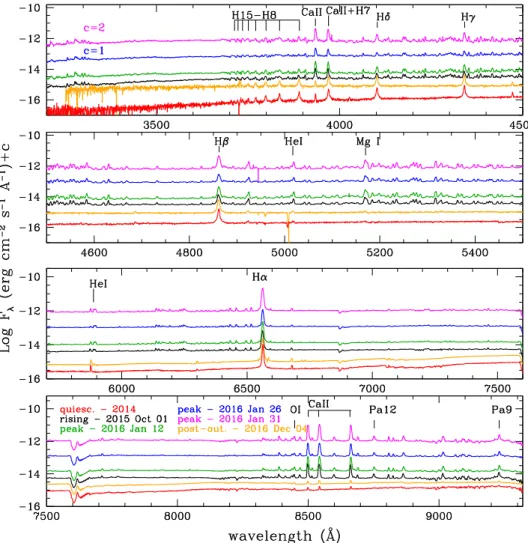
In Figure 3 the four MODS spectra are depicted in

comparison with the quiescence spectrum (Paper I) and that

obtained during the rising phase(PaperII). The same forest of

lines asobserved in the 2015 October spectrum is present in

the burst spectra, but further increased in brightness. The large majority are recombination lines or lines of neutral and ionized metals (HI, HeI, CaII, FeI, andFeII), most of them blended

with each other. We give in Table5the linefluxes of bright and unblended lines that are used in the spectral analysis. Theirflux is computed by integrating the signal belowthe spectral profile.

The FWHM is compatible with the instrumental one

becau-sethe lines arenot resolved in velocity at the adopted

resolution. The associated uncertainty is estimated by evaluat-ing the rms in a wavelength range close to the line, and then multiplying it by the FWHM.

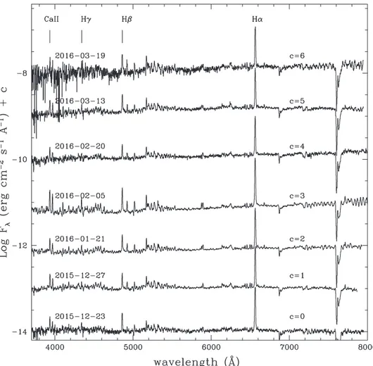
The low-resolution Asiago spectra are shown in Figure 4.

Together with HI and CaII lines, other features of metallic

lines are prominent in the spectrum, but they result from blends

of two or more lines, so their flux is notuseful for the line

analysis.

Most of the permitted lines that appear blended in the optical

low-resolution spectrum are clearly identified at the spectral

resolution achieved in the echelle spectra. A list and comments on these lines are provided in AppendixAand in Section3.2.4, respectively. Profiles of the most interesting lines (in particular theBalmer lines) are presented in Section3.3.

Table 4

Journal of Spectroscopic Observations

Date MJD Telescope/Instrument _Dl R rms Exp Time

(Å) (10−16_{erg s}−1_cm−2_Å−1_{) (s)} 2015 Dec 23 57379 1.22 m/B&C 3300–8050 2400 7–12 1800 2015 Dec 23 57379 1.82 m/ECH 3600–7300 20,000 7–20 1800 2015 Dec 27 57383 1.22 m/B&C 3300–8050 2400 4–7 3600 2015 Dec 27 57383 1.82 m/ECH 3600–7300 20,000 7–25 1800 2015 Dec 29 57385 1.82 m/ECH 3600–7300 20,000 4–13 3600 2016 Jan 10 57397 TNG/GIANO 9500–24 500 50,000 – 3000 2016 Jan 12 57399 LBT/MODS 3200–9500 1500 0.9–1.2 1500 2016 Jan 21 57408 1.82 m/ECH 3600–7300 20,000 15–38 3600 2016 Jan 21 57408 1.22 m/B&C 3300–8050 2400 3–6 3600 2016 Jan 25 57412 LBT/LUCI2 10,000–24,000 1000 0.7–1.6 1200 2016 Jan 26 57413 LBT/MODS 3200–9500 1500 0.9–1.1 1500 2016 Jan 31 57418 LBT/MODS 3200–9500 1500 0.7–1.0 1500 2016 Feb 05 57423 1.22 m/B&C 3300–8050 2400 4–7 3600 2016 Feb 20 57438 1.22 m/B&C 3300–8050 2400 2–6 5400 2016 Feb 20 57438 1.82 m/ECH 3600–7300 20,000 12–41 3600 2016 Mar 02 57449 LBT/LUCI2 10,000–24,000 1000 1.1–2.2 1200 2016 Mar 13 57460 1.22 m/B&C 3300–8050 2400 10–20 900 2016 Mar 19 57466 1.82 m/ECH 3600–7300 20,000 12–42 1800 2016 Mar 19 57466 1.22 m/B&C 3300–8050 2400 8–20 2400 2016 Apr 05 57483 TNG/GIANO 9500–24 500 50,000 – 3000 2016 Oct 04 57665 LBT/LUCI2 10,000–24,000 1300 0.7–2.0 1200 2016 Dec 04 57726 LBT/MODS 3250–9500 1500 0.7–1.0 1500 11 http://www.iasf-milano.inaf.it/Research/lbt_rg.html 12

IRAF is distributed by the National Optical Astronomy Observatory, which is operated by the Association of the Universities for Research in Astronomy, inc. (AURA) under cooperative agreement with the National Science Foundation.

Fluxes of unblendedbright lines observed with the Asiago telescopes are listed in Table6. The sensitivity limit is about a factor of ten lowerthan the limit of MODS, therefore reliable fluxes can be given only for some permitted lines (not reported in Table6), along with theBalmer and CaIIH lines. Whenever both a low- and a high-resolution spectrum is available at a

certain date, thefluxes agree each other within 20%, with the

exception of theflux of Hα, which shows prominent wings that

are better resolved at higher dispersion. In Table 6 we

thereforegive the average of the two determinations, except

for Hα, for which we report the flux measured in the

high-resolution spectrum.

Finally, we note that many lines present a remarkable level of variability on timescales of days(see Tables 5 and 6). For

example, Hα and Hβ fluxes increase byabout a factor of two

from January 26 to 31. As we show as an example in the

bottom panel of Figure 2, the variation of F(Hβ) roughly

follows that of the continuum, although with a certain delay. In particular, thecontinuum fades faster than thelines. This is

evident for the last spectroscopic point(MJD 57726), when the

continuum level was close to that of quiescence (top panel),

while F(Hβ) was still about a factor of 5 brighter.

Thiscircumstance appears to be a common feature of EXor

variability(Paper I).

2.3.2. Near-IR Spectroscopy

Three near-infraredlow-resolution spectra have been

obtained with the LUCI2 instrument at LBT on 2016 January 25, March 2, and October 4. The observations were carried out with the G200 low-resolution grating coupled with the 1 0 slit

on thefirst two dates and with the 0 75 slit on October 4. The

standard ABB’A’ technique was adopted to perform the

observations using the zJ and HK grisms, for a total integration

time of 12 and 8 minutes, respectively. The final spectrum

covers the wavelength range 1.0–2.4 μm atR ~1000. Data

reduction was performed at the Italian LBT Spectroscopic

Reduction Center. The raw spectral images were flat-fielded,

sky-subtracted, and corrected for optical distortions in both the spatial and spectral directions. Telluric absorptions were removed using the normalized spectrum of a telluric standard star, afterfittingits intrinsic spectral features. Wavelength

calibration was obtained from arc lamps, whileflux calibration

was achieved through observations of spectrophotometric

standards, carried out inthe same night as the target. No

Figure 3.Optical(LBT/MODS) spectra of V1118 Ori taken in 2016 January (peak: green, blue, and pink) and 2016 December (post-outburst: orange), shown in comparison with the spectra taken in quiescence(red, PaperI) and during the rising phase (black, PaperII). For a better visualization a constant (indicated in the top

panel) was added to the spectra taken on January 26 and 31. Main emission lines are labeled.

intercalibration was performed between the zJ and HK parts of

the spectrum, since they wereoptimally aligned. We evaluated

possible flux losses by comparing the continuum level at the

JHK effective wavelengths (1.25, 1.60, and2.20 μm) with the

magnitudes of the closest photometric points, obtained within a

week from the spectroscopic observations. While for the first

two spectra(January 25 and March 2), the agreement is within

20%, significant flux losses, mainly due to the bad weather

conditions during the observation, are registered in the

spectrum of October 4. Thereforewe used the photometric

data of October 1 to calibrate this spectrum, whichin any case

ismuch fainter than the first two. No intercalibration was

applied between near-IR and optical spectra as they all were acquired on different dates.

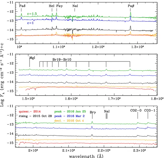
The three LUCI2 spectra are shown in Figure 5, in

comparison with the spectra taken in quiescence (Paper I)

and during the rising phase (Paper II). Fluxes of the main

unblended lines are listed in Table 7. In the peak phase the

most prominent lines are HI recombination lines of the

Paschen and Brackett series, HeI1.08μm, MgI, and NaIlines. CO 2-0 and 3-1 ro-vibrational bands are also observed in emission. Other metallic lines are likely present, but they are too faint or strongly blended to be clearly identified. In the last spectrum, taken during the declining phase, we detect the

brightest HI lines, HeI 1.08μm, and H22.12μm. Notably,

while HIlinefluxes are similar to those during the rising phase (PaperII), the continuum level is closer to the quiescence level.

This confirms what we have already noted about the optical

lines in Section2.3.1.

Near-IRhigh-resolution spectra were obtained on 2016

January 10 and 2016 April 05 with GIANO at the Telescopio

Nazionale Galileo (La Palma. Spain) during two Director

Discretionary Time (DDT) runs. GIANO

providessingle-exposure cross-dispersed echelle spectroscopy at a

resolu-tion of 50,000 (δv∼6 km s−1 at λ=1 μm) over the

0.95–2.45 μm spectral range. Since at longer wavelengths

the echelle orders become larger than the 2k×2k detector,

the spectral coverage in the Kband is 75%, with gaps, for

example, at the Brγ and CO 1-0 wavelengths. GIANO is

fiber-fed with two fibers of 1″ angular diameter at a fixed

angular distance of 3″ on sky. The science target is acquired

by nodding on fiber, namely alternatively acquiring target

and sky on fibers A and B, and viceversa. This allows an

optimal subtraction of the detector pattern and sky

back-ground. Data reduction was achieved by means of specific

scripts optimized for GIANO.13 In particular, observations

of a uranium-neon lamp were carried out to perform

wavelength calibration, while flat-fielding and mapping of

the order geometry were achieved through exposures with a tungsten calibration lamp. The reduced spectrum is rich in metallic lines that were barely detected in the low-resolution

spectrum, which we list in AppendixBand comment on in

Section3.2.4. Profiles of the most interesting lines (HIlines

and HeI1.08μm) are presented in Section3.3.

Table 5

Fluxes of Main Lines Detected with LBT/MODS

2016 Jan 12 2016 Jan 26 2016 Jan 31 2016 Dec 04

Line lair Flux±Δ Flux

(Å) (10−15_{erg s}−1_cm−2₎ H15 3711.97 10.5±1.8 L 15.8±2.0 L H14 3721.94 14.3±1.8 9.9±0.9 18.8±2.0 L H13 3734.37 18.7±1.8 12.2±1.1 23.9±2.0 L H12 3750.15 21.7±1.8 12.7±1.1 25.5±2.0 2.1±0.7 H11 3770.63 20.4±1.8 11.6±1.1 22.4±2.0 3.1±0.7 H10 3797.90 21.9±1.8 10.9±1.1 31.6±2.0 4.9±0.7 H9 3835.38 32.8±1.8 10.7±1.1 32.5±2.0 6.3±0.7 H8 3889.05 29.6±1.8 10.3±0.9 33.0±2.0 9.5±0.7 CaIIH 3933.66 105.92±1.7 73.3±1.0 170.3±2.0 3.5±0.7 CaIIK+ H7 3968.45/3970.07 99.2±1.7 55.3±1.0 152.4±2.0 14.1±0.7 HeI 4026.19 9.2±1.7 6.5±1.0 9.8±2.0 L Hδ 4101.73 50.4±1.7 28.3±1.0 75.7±2.0 17.15±0.4 Hγ 4340.46 71.9±1.7 42.0±1.0 96.8±2.0 20.3±0.4 Hβ 4861.32 186.11±1.7 112.6±1.0 231.3±2.0 31.1±0.2 HeI 5015.68 16.18±1.7 12.0±1.0 14.1±2.0 1.4±0.2 MgI 5168.76/5174.12 27.8±1.7 36.2±1.7 20.2±1.0 L MgI 5185.05 7.3±1.7 10.2±1.7 5.4±1.0 L HeI 5875.6 27.1±1.8 13.5±1.1 29.5±2.0 3.5±0.2 [OI] 6300.30 15.5±1.8 9.5±1.2 11.7±2.0 15.75±0.2 Hα 6562.80 1546.8±2.0 765.0±1.2 1635.5±2.0 149.4±0.2 HeI 6678.15 23.9±2.0 14.5±1.2 23.2±2.0 2.8±0.2 HeI 7065.2 15.8±2.0 10.3±1.2 14.3±2.0 L OI 8446.5 59.6±2.0 34.4±1.1 51.9±2.0 4.5±0.2 CaII 8498.03 572.8±2.0 372.3±1.0 526.8±2.0 9.1±0.2 CaII 8542.09 670.5±2.0 430.7±1.0 636.5±2.0 8.0±0.2 CaII 8662.14 584.9±2.0 370.6±1.0 546.2±2.0 8.4±0.2 Pa12 8750.47 97.0±2.0 64.3±1.3 75.4±2.0 L Pa9 9229.01 183.7±2.0 89.3±1.3 144.5±2.0 5.2±0.2 13

GIANO_TOOLS, available at the TNG webpage(http://www.tng.iac.es/

3. Analysis and Discussion 3.1. Photometric Analysis

3.1.1. Light Curve

The 2015–2016 outburst is the sixth documented during the

recent history (about 40 years) of V1118 Ori; previous events

(1983, 1989, 1992, 1997, and2005) are recognizable in the

lightcurve in Figure 1. Thisglobal view of the V1118 Ori

photometric behavior shows two facts:(1) the present outburst

is roughly at the same intensitylevel(Vpeak~13.5mag) and

duration (∼1 year) as the bursts thatoccurred between 1989

and 1997, whereas theoutburstin 2005 has been the brightest

(Vpeak~12mag) and maybe the longest(2 years); (2) in the course of time the monitoring improved progressively in both sampling cadence and spectral coverage. In particular, systematic observations have shown that V1118 Ori has

remained quiescent for about a decade (from 2006 to 2015).

Indeed, four out of the five previously known events have

occurred with a roughly regular cadence of 6–8 years, withthe only exception the outburstin 1992 (Garcia Garcia et al.1995),

which wasmuch fainter than all the others ( V 14.7 mag),

however. The evidence that the 2015 outburst is not in phase

with the previous outbursts does not supportperiodic

phenom-ena as the cause of the outburst triggering. Aquiescence period

of about 15 years(from 1966 to 1981) has alsobeen shownby

a recent analysis of historical plates (Jurdana-Šepić et al.

2017a).

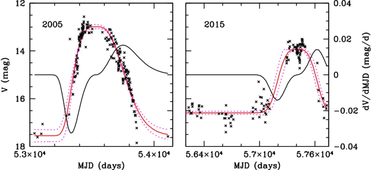
We have compared the present outburst with the outburstof

2005to understand whether they have followed a similar

evolution in time. In Figure 6the V lightcurves of the 2005

and 2015 outbursts are shown in the left and right panel, respectively. While the 2005 outburst has occurred as a sudden Figure 4.Optical low-resolution spectra of V1118 Ori taken with the 1.22 m Asiago telescope during the peak phase. For a better visualization a constant was added to theflux density. Main emission lines are labeled.

Table 6

Fluxes of Lines Detected with the Asiago Telescopes

Date Flux a_{±ΔFlux (10}−15_{erg s}−1_cm−2₎ a H b Hβ Hγ Hδ CaIIH 2015 Dec 23 1259±19 162±18 71±22 54±20 89±20 2015 Dec 27 1070±16 142±18 69±20 51±20 68±25 2015 Dec 29c _{1291±18 172±19 74±20 71±20 74±20} 2016 Jan 21 1129±19 197±20 97±24 50±20 84±20 2016 Feb 05d _{1076±12 177±12 58±17 L L} 2016 Feb 20 1051±18 118±18 64±20 L 86±25 2016 Mar 13d 1110±30 189±30 63±23 L L 2016 Mar 19 1056±18 115±18 52±20 L L Notes. a

Fluxes are the average of the values measured in the low- and high-resolution spectrum, unlessspecified otherwise.

b

Flux measured in the high-resolution spectrum(see text).

c

On this date, only a high-resolution spectrum is available.

d

On this date, only a low-resolution spectrum is available.

Figure 5.Near-IRLUCI2 spectra taken on 2016 January and March (peak: green, blue), and 2016 October (declining: orange) in comparison with spectra taken in quiescence(red, PaperI) and during the rising phase (black, PaperII). For a better visualization a constant (indicated in the top panel) was added to the spectra taken

on January 25 and March 2. Main emission lines are labeled.

Table 7

Fluxes of Main Lines Detected with LUCI2

2016 Jan 25 2016 Mar 02 2016 Oct 04

Line lair Flux±Δ Flux

(Å) (10−15_{erg s}−1_cm−2₎ Paδ 10049.37 238.1±2.0 181.5±2.0 40.0±2.0 HeI 10830.3 (−32.2) 79.8±2.0 (−18.0) 113.8±2.0 (−3.5) 7.2±0.3 Paγ 10938.09 274.9±2.0 196.2±2.0 65.3±1.0 NaI 11406.90 27.9±3.0 32.6±3.0 L Paβ 12818.08 362.5±2.0 282.8±2.0 71.8±1.0 MgI 15029/15051 75.6±4.0 52.3±3.0 L Br19 15264.71 26.8±4.0 23.4±3.0 L Br18 15345.98 27.7±4.0 26.8±3.0 L Br17 15443.14 34.3±4.0 34.0±3.0 L Br16 15560.70 31.2±4.0 36.8±3.0 L Br15 15704.95 41.0±4.0 37.4±3.0 L Br14+OI 15885/15892 111.4±4.0 97.3±3.0 L Br13 16113.71 51.1±4.0 47.6±3.0 L Br12 16411.67 72.0±4.0 72.0±3.0 L Br11 16811.11 73.4±4.0 75.1±3.0 15.6±3.0 Br10 17366.85 84.9±4.0 80.0±3.0 10.1±3.0 H21-0S(1) L L L 3.9±0.7 Brγ 21655.29 83.8±4.0 75.6±3.0 15.5±0.7 NaI 22062.4 17.5±4.0 10.0±3.0 L NaI 22089.7 10.9±4.0 9.9±3.0 L CO 2-0 22943 185.1±10.0 140.8±10.0 L CO 3-1 23235 161.7±10.0 117.9±10.0 L

event starting from a very faint level ( V 17.5 mag), the outburstof 2015 followed a long period that wascharacterized

by ahigher average brightness (á ñ ~V 16.5 mag) with daily

scale fluctuations of several tens of magnitude, presumably

unrelated with the accretion burst. Quantitatively, the two

lightcurves (covering about 1200 days each) have been fitted

with a single distorted Gaussian.14 This is depicted as a red

solid curve, while the fit uncertainty is represented with pink

dotted lines. The derivative to the fitted Gaussian (black line) allows us to account for the speed typical of the different outburst phases. In 2005, the rising speed has increased

monotonicallyto values (∼0.035 mag/day) about twicethe

decreasing speed(∼0.015 mag/day). Notably, the 2015

out-burst is characterized by a similar rising and declining speed (∼0.015 mag/day). This might indicate thatwhile triggering has occurred under different modalities, the relaxing phenom-enon has followed as similar evolution.

In conclusion, as also confirmed by spectroscopic data, see

Section 3.2.2, the 2015 outburst appears different from the

outburst in 2005, as far as intensity, duration, recurrence time,

and rising speed are concerned. Whetherthe observed behavior

is specific of V1118 Orior ismore in general a common

feature of the EXor variability, remains an open question. For the moment, the possible comparison is with the candidate EXor V2492 Cyg, which shows a slower rising than declining phase, although the variability of this source is not fully due to

disk-accretion phenomena(Hillenbrand et al. 2013).

3.1.2. Color Analysis

To investigate the origin of the photometricfluctuation, we

plot in the left panel ofFigure 7the optical[V-R versus]

-[R I colors of V1118 Ori measured during quiescence and]

recent outbursts (2005 and 2015). These are obtained by

combining the data of the present paper with those by Audard

et al. (2010). Quiescence and outburst phases areidentified

byV lower orgreater, respectively,than 15 mag. The data

points of the 2015 outburst follow a similar distribution as

those of 2005. As has beenshown by Audard et al. (their

Figure 11), colors become bluer with increasing brightness,

moving almost parallel to the reddening vector in the direction of a decreasing extinction. However, although a variable extinction certainly plays a role (see also Section 3.2.1), it cannot be the primary cause of the brightness enhancement typical of outbursts. Indeed, as shown in thefigure, the colors of an unreddened main-sequence star of the V1118 Ori spectral

type (M1–M3) are typically redder than the outburst colors.

Instead, and in agreement with previous studies on EXors (Audard et al. 2010; Lorenzetti et al. 2012), we interpret the blueing of the optical colors as mainly due to a hotter temperature component appearing during the outburst. Note that in this view the extinction may even increase during outburst, but not enough to compensate for the blueing of the color indices.

The near-IR [J-H] versus [H-K] color diagram

(Figure 7, right panel) is in agreement with the above

interpretation. Indeed, although colors of the different phases

(quiescence: H11, outburst: H<11) spread over a large

portion of the plot, they roughly segregate into two different portions of the plot, whose connecting direction does not follow that of the reddening vector.

3.2. Line Analysis

3.2.1. Extinction Estimate

As a first step of the line analysis, we have estimated the

extinction toward V1118 Ori. A common and powerful tool to

achieve thisis to use pairs of optically thin and bright

transitions coming from the same upper level, since in this

case the difference between observed and theoreticalflux ratio

Figure 6.Left panel: V lightcurve of the 2005 outburst. The red solid curve is the best distorted Gaussian through the data points, whose uncertainty is represented by the pink dotted lines. The black solid line is the derivative of the distorted Gaussian, which represents the velocity in magnitude variation. Right panel: the sameas in the left panel for the 2015 outburst. A large portion of the lightcurve before the outburst is plottedto show the quiescence level.

14_{Represented as y x( )~exp}-f x(, , ,ss k)2_{, with σ=standard deviation,}

s=skewness, andk=kurtosis.

depends only on the extinction value. We have considered pairs

of HI lines whose profiles do not seem affected by evident

opacity effects, such as self-absorption or flatted peaks (see

Section3.3). These arePaβ/Hγ, Paγ/Hδ, Pa9/H9, Pa12/H12,

and Brγ/Paδ. Considering all the available spectra, we estimate

AV in the range 1.5–2.9 mag, without any significant trend

between quiescence and outburst phases. Indeed, extinction fluctuations ofup to 1 mag are also recognizablein the color– color diagrams of Figure 7.

As analternative method, we estimate AVby modeling and

fitting the uv/optical MODS continuum (Section 3.2.2). In

good agreement with the range found from line ratios, the best

fit provides AV=2.9 mag in quiescence, rising, and at the

outburst peak, and AV=1.9 mag in the post-outburst phase.

For comparison, our AVestimate is also compatible with that

between 1.4 and 1.7 mag obtained by Audard et al.(2010) on

the basis of X-rayobservations during the outburst of 2005. Summarizing, since our analysis is largely based on the uv/ optical lines and continua, an AVintrinsic variability of about

1 mag might significantly reflect on the estimate of physical

parameters and mass accretion rate. Therefore, in the following

we consider conservativelythe two extreme values of AV,

namely 1.5 and 2.9 mag. This will give us an idea of how much the AVvariability influences the results.

3.2.2. Mass Accretion Rate

To determine the mass accretion rate( ˙Macc) we applied two

different methods (indeed not strictly independent) involving

both continuum and emission lines.

In the first method, described in Manara et al. (2013), we

fitted the observed MODS spectrum in various continuum

regions from ∼3200Å to ∼7500Å using the sum of a

photospheric template and a slab model to reproduce the continuum excess emission due to accretion. We adopted the reddening law by Cardelli et al.(1989) with RV=3.1. We first fitted the quiescence spectrum taking as free both the stellar parameters and the extinction value. The bestfit (Figure8, top panel)is obtained with a photospheric template of spectral type (SpT) M3 and for AV=2.9 mag (as anticipated in the previous section). These lead to *R =1.67 RandL =0.32Lwhen

a distance of 414 pc is adopted. By assuming the evolutionary

models of Baraffe et al. (2015), the fitted parameters

correspond toM_*=0.29 M. According to our working plan,

we alsofitted the quiescence spectrum adopting AV=1.5 mag

(not shown in the figure). The fit gives SpT=M3, *R =1.07

R, L_å=0.18 L_e, andM_*=0.29 M.

Fits of the subsequent phases (rising, peak, and

post-outburst, Figure8, second, third, and fourth panel) were made

by assuming the stellar parameters fitted in quiescence, and

keeping AV and SpTfixed. We varied the contribution of the

slab to the emission until a bestfit was found. This is the same

procedure as adopted tofit DR Tau by Banzatti et al. (2014).

The fit of the rising and peak spectra, in particular, is very

uncertain becausethe continuum emission is dominated by the

accretion shock. The ˙Macc derived with this“continuum” (C)

methodare listed in Table8,first and second column. As a second method, we applied the empirical relationships

derived by Alcalá et al. (2016) between line and accretion

luminosity(Lacc) for a sample of young active T Tauri stars in

Lupus. We assumed the same parameter values as for the

continuumfitting, which were also taken to recompute the mass

accretion rate in quiescence and rising phases(given in PapersI andII). This allows us to meaningfully compare the results. We applied the Alcalá et al. relationships to the brightest HIlines (those detected with a S/N10), which are the Balmer lines Figure 7.Left panel: optical two-color plot[V-R vs.] [R-I . Orange] /red crosses: quiescence data ( V 15) in the periods 2007–2010/2013–2015; teal-blue/blue crosses: 2005/2015 outbursts data ( <V 15). References: present paper; Audard et al. (2010). Dotted line: unreddened main-sequence. Colors of M1 and M3 stars are

indicated. Arrow: extinction vector corresponding to AV=1 mag (reddening law of Cardelli et al.1989). The average error is indicated with a black cross. Right

panel: the sameas in the left panel for the near-IR two-color plot[J-H vs.] [H-K . Quiescence and outburst are de] fined asH11 andH<11, respectively. References: present paper; PapersI,II; Audard et al.(2010). Dashed line: locus of the T Tauri stars (Meyer et al.1997).

in the MODS and Asiago spectra, and the Paschen and Brγ lines in the LUCI2 spectra.15 Finally, we converted Laccinto

˙

Maccbyapplying the relationship reportedby Gullbring et al.

(1998). The results are summarized in Table8, third and fourth

column (“Line” (L) method).

The ˙Maccvalues are also shown in Figure9, where different

colors are used to represent the adopted fitting method and

extinction value. M˙acc increased byabout two orders of

magnitude from quiescence to the outburst peak, going from 0.3–2.0 10−8Myr−1to 0.2–1.9 10−6Myr−1. The upper end

value is close to the estimate by Audard et al. (2010) at the peak of the 2005 outburst, obtained by means of spectral

energy distribution(SED) fitting. Given the higher brightness

attained by the 2005 outburst, its mass accretion rate should presumably be higher than for the 2015 event.

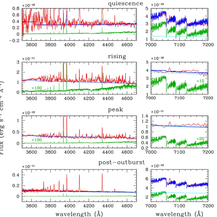
Figure 8.Top panel: dereddened spectrum(AV=2.9 mag) of V1118 Ori between 3500–4700Å and 7000–7200Åduring quiescence (red). The spectrum of an M3

star template is shown in green. The continuum excess emission of the slab model is plotted in cyan, while the bestfit with the emission predicted from the slab model added to the template is given by the blue line. Other panels: the sameas in the top panel for the rising, peak, and post-outburst phases. In this latter, the spectrum was dereddened for AV=1.9 mag. For a better visualization, the template spectrum has been multiplied by a constant where indicated.

15

We avoid usingthe Hα line, as suggested by Alcalá et al., because self-absorption features and multiple components, likely arising from gas that isnot strictly related with the accretion columns, strongly affect the observed profile (see Section3.3).

For a fixed AV, the ˙Macc derived with the two methods is

consistent within the uncertainties, withthe only exception that of the rising phase; conversely, differences ofup to a factor of

four are found between M˙acc derived under a different AV

assumption. Since these differences are due to the intrinsic short-timescale variability of V1118 Ori, and not to a poor

determination of AV, the extreme M˙acc values have to be

considered as the lower and upper end values that characterize the considered temporal phase.

Finally, it is also interesting to note that M˙acc

(post-outburst)≈ ˙Macc(rising), even if the continuum level is very

close to the quiescence value. This result is a direct

consequence of the slower decrease of the line fluxes, as we

have shown in Figure2for the case of the Hβ flux.

3.2.3. Hydrogen Physical Conditions

To derive the physical conditions of the gas thatemitsthe

HIlines, we have compared the observed Balmer decrements

(plots of flux ratios versus upper level of the transition) with the predictions of the local line excitation computation by Kwan &

Fischer (2011), who provide a grid of models in the range of

hydrogen density log [nH (cm−3)]=8–12 and temperature

Table 8 Mass Accretion Rate

Phase M˙acc(Myr−1)a C-1.5 C-2.9 L-1.5 L-2.9 Quiescenceb _{3.1±1.0 10}−9 _{2.0±0.7 10}−8 _{3.5±2.5 10}−9 _{1.6±1.1 10}−8 Risingc _{1.1±0.4 10}−7 _{6.8±2.4 10}−7 _{4.2±0.8 10}−8 _{3.1±0.5 10}−7 Peakd 3.2±1.1 10−7 1.9±0.7 10−6 2.0±1.0 10−7 9.6±3.1 10−7 Declininge L L 8.0±2.2 10−8 1.4±0.5 10−7 Post-outburstf 3.0±0.4 10−8 6.4±0.4 10−8 2.6±0.9 10−8 1.8±0.8 10−7 Notes. a

Column labels refer to the method(C: “continuum,” L: “lines”) and to the adopted AV(1.5 and 2.9 mag).

b

Derived from data of PaperI(taken in 2014).

c

Derived from data PaperII(taken in 2015 October).

d

Average of the determinations between 2015 December and 2016 March.

e

Measured on the LUCI2 spectrum taken in 2016 October.

f

Measured on the MODS spectrum taken in 2016 December.

Figure 9.Mass accretion rate as a function of time. With different colors we depict ˙Maccvalues derived under different assumptions for thefitting method or the

adopted extinction. Determinations of ˙Maccthat refer to 2014 August–December and 2015 October have been obtained from the spectra published in PapersIandII,

between 3750 K and 15,000 K. We have also examined the Paschen decrements for the few lines we observe, and

compared them with the models by Edwards et al. (2013).

We show the results in Figure10, where Balmer(from MODS

spectra) and Paschen (from LUCI2 spectra) decrements are

represented in the largepanels and the insets, respectively.

Since the Hα line can be severely contaminated by opacity

effects and chromospheric emission, we preferred to use the Hβ

as a reference line for the Balmer decrements(e.g., Antoniucci

et al. 2017). Furthermore, as the decrement shape may vary

depending on the adopted reference line, we have verified that

using lines with a higher nup as reference does not provide

significantly different results from thosereported here. The

Paschen decrements have been normalized to the Paβ line.

Balmer decrements during the quiescence phase are shown in the top panels, after they have been corrected for Figure 10.Balmer decrements(Hi/Hβ flux ratios vs. upper level of the transition) in quiescence (top panels), rising/peak (central panels), and post-outburst phases

(bottom panels). In the left and right panels the observed ratios are corrected for AV=1.5 mag and 2.9 mag, respectively. The fluxes have been normalized to the Hβ

flux. The observations have been fitted with the local line excitation models of Kwan & Fischer (2011). Models with different temperatures are depicted with different

colors, and the adopted density is labeled. In the insets, the Paschen decrements(normalized to the Paβ) are shown and compared with the relative predictions of Edwards et al.(2013).

AV=1.5 mag (left) and AV=2.9 mag (right). Regardless ofthe adopted extinction value, the decrement shape resembles the straighttype 2 shape cataloged by Antoniucci et al. (2017). To this class of decrements typically belong T Tauri sources with ˙Maccin the range −10.8<log [ ˙Macc(M yr−1)]<−8.8,

in good agreement with our estimates of Section3.2.2. Forthe twoAVvalues, wefind that models with log [nH(cm−3)]=9.4

are those that best fit the observed decrements, even if the

overall shape is not well reproduced. No significant constraint

can be placedon the hydrogen temperature from the Balmer

decrements alone. While lower temperatures seem favored

whenAV=1.5 mag is adopted, the opposite occurs for

AV=2.9 mag. The Paschen decrements, although not well

fitted by models16

, suggestT10,000 K.

In the central panels we show the Balmer decrements of the rising(triangles) and peak (circles) phases. The most important difference with respect to quiescence is the enhancement of the ratios of lines with nup10 of at least an order of magnitude.

Whencompared with the decrementclassification of

Anto-niucci et al., rising and peak decrements resemble the

L-shapetype4decrements, observed mostly in objects with log

[ ˙Macc(M yr−1)] > −8.8. Again, according to the Kwan &

Fischer models, the hydrogen density has increased by about two orders of magnitude with respect to quiescence, while temperatures between 8750 and 15,000 K are suggested by both the Balmer and Paschen decrements.

In the bottom panels we showthe Balmer decrements of the

post-outburst phase. Their shape is of type 3, or bumpy, accor-dingto the definition of Antoniucci et al., which is intermediate between types 2 and 4 (−9.8<log [ ˙Macc(M yr−1)]<−8.8).

A good agreement between models and data is found only for log[nH(cm−3)]=9.6, T 10,000 K and AV=1.5 mag.

We can conclude that the physical conditions of the gas

profoundly changedfrom quiescence to outburst, and this is

especially true forthe gas density. We can argue that this has led also to a similar enhancement in the accretion column density and consequently in the mass accretion rate.

3.2.4. Other Lines

The high-resolution Asiago (echelle) and TNG (GIANO)

spectra display a number of unblended emission lines of neutral atoms typical of M-type stars(e.g., Na, Ca, Fe, Ti, andSi, see AppendicesAandB). Because of their low-ionization potential (between 5 and 8 eV), these lines likely originate in neutral regions close to the disk surface, far enough from the central star and accretion columns to prevent their ionization, butstill reached by stellar UV photons able to populate energy levels

close to the continuum, however. In Table 9 we listfor each

metallic speciesthe energy of the most highly excited line, max (Eup), and the number of detected lines, Nlines. The reported

statistics is done considering only the optical lines (in the

3300–7300Å range covered at highresolution), since this

allows a meaningful comparison with the optical spectrum of EX Lup, taken during its 2008 outburst by Sicilia-Aguilar et al. (2012). As we show in the last two columns of Table9, the EX Lup spectrum is definitely richer inhigh-excitation lines. This suggests that in this source the accretion shock produces more energetic photons or that the radiation shielding is less efficient

in its environment. It isinteresting, however, thatin contrast to

this general trend, much more highly excited lines of TiIand

VIare detected in V1118 Ori. Very likely, both these species

are almost completely ionized in EX Lup, given their low-ionization potential(6.8 eV for TiIand 6.7 eV for VI). Finally,

we reportthe detection of LiI6707Å in emission (S/N ∼4), a feature that is alsopresent in the outburst of 2005 (Herbig 2008). This line is usually absent or seen in absorption in the spectra of classical T Tauri stars.

It is interesting to perform a more in-depth study of the FeI

lines thatdominate the emission spectrum during the outburst.

For this study we have considered all the FeI lines predicted

bytheory with λ between 4000 and 20000Å and inside the

atmospheric windows, but discarding those with A Einstein

coefficients „103s−1 or energy of the upper level

Eup…7.15 eV. The atomic data (Acoefficients, statistical

weights, and Eup values) are taken from “The atomic line

list,” v.2.05b21,http://www.pa.uky.edu/~peter/newpage/. In

Figure11we plot as black crosses the theoretical product gijAij (statistical weight timesEinstein coefficient) of the FeIlines as

a function of Eup. This product is proportional to the line

intensity, and therefore it gives an idea ofthe brightest lines depending on the level of the gas excitation. With red crosses we indicate the lines observed in V1118 Ori. Although with exceptions, we observe the lines having gijAij5 105s−1for Eup6.5 eV and gijAij107s−1for Eup6.5 eV. We do not

observe lines having Eup> 6.7 eV, a value in between the

maximum Eup of lines observed in DR Tau (in quiescence,

Beristain et al.1998) and in EX Lup (during outburst, Sicilia-Aguilar et al.2012).

Indications of the temperature and density of the line-emitting regions can be derived from theratios of bright lines.

The three CaII emission lines at λλ8498, 8542, and 8662Å

remained roughly constant throughoutthe outburst duration

with ratios close to unity, which are suggestive of optically Table 9

Statisticsa_{of the Optically Permitted Lines}

Element IPb V1118 Ori EX Lup

max(Eup)b Nlines max(Eup)b Nlines

LiI 5.39 1.8 2 L L NaI 5.13 2.1 2 4.9 3 MgI 7.64 5.1 1 7.6 10 SiI 8.15 5.1 1 7.5 7 SiII 16.34 10.1 2 14.8 6 CaI 6.11 4.5 15 5.7 27 CaII 11.87 3.1 2 10.0 3 TiI 6.82 6.0 15 3.9 6 TiII 13.57 5.6 21 5.6 43 VI 6.74 5.4 10 4.7 4 CrI 6.76 5.0 11 5.0 31 CrII 16.49 6.8 5 6.8 12 FeI 7.87 6.7 112 7.2 >400 FeII 16.18 5.9 39 8.2 ∼70 CoI 7.86 4.0 2 4.2 9 NiI 7.63 4.1 4 6.1 17 Notes. a

The comparison between V1118 Ori and EX Lup spectra has been made within the range 3300−7300Å covered with the echelle of the 1.82 m Asiago telescope.

b

Units are eV.

16

Note that we consider Paschen models at log[nH(cm−3)]=9.0 and log [nH

(cm−3_{)]=11.4 for quiescence and rising/peak, since models at the same}

thick environments. According to the analysis of a sample of Herbig stars, Hamann & Persson (1992) have estimated that CaIIoptically thick lines are produced for anelectron density of 1011cm−3 and ahydrogen column density …1021cm−2, if the temperature is between 4000 and 10,000 K. Indeed, we can set as upper limit the maximum hydrogen temperature of ∼15,000 K derived from the analysis of the Balmer lines

(Section 3.2.3), and as a lower limit the few thousandKelvin

(typically 4000 K) that are typically traced by the emission of

the CO ro-vibrational bands(see below).

Other remarkable lines are the OItriplet at 1.29μm, pumped

by the Lyβ (McGregor et al. 1988), and whose de-excitation

originates the 8446 Å, and the NaI 2.206, 2.207μm doublet.

Lorenzetti et al. (2009, their Figure 14) noted that in EXor

spectra the NaI doublet is detected both in emission and in

absorption following the same behavior of the CO bands. Usually, strong CO emission is seen during outburst phases, while a progressive fading, absence, or absorption is detected

as the outburst proceeds toward quiescence (e.g., Aspin

et al. 2008 and references therein; Biscaya et al. 1997;

Hillenbrand et al. 2013). This is alsoseenin V1118 Ori:

neitherquiescent nordeclining spectra showCO bands or the

NaIdoublet, while in outburst bothspecies are seen in

emission (Figure 5). The common origin of CO and NaI

emission is likely due to the very low-ionization potential of

neutral sodium(5.1 eV), which can survive only close to

low-mass late-type stars(like EXor, T Tauri, e.g., Antoniucci et al.

2008), andmore generally, in regions deep enough inside the

circumstellar disks where CO ro-vibrational bands are collisionally excited and shielding against photons that areable

to produce Na+ is efficient (McGregor et al. 1988). These

conditions require densities >107cm−3 and only moderately

warm temperatures, becauseCO iscompletely dissociated at

∼4000 K.

The [OI] 6300 Å line is the only forbidden optical line

present in the V1118 Ori spectrum(at an S/N∼6–8). In the

Asiago high-resolution spectra, the line presents a structured

profile that can be deconvolved into two components, one close

to the peak of the diffuse [OI] 6300 Å in the Orion nebula

(vhelio~ +30km s−1, García-Díaz & Henney 2007), and a blueshifted component centered atvhelio~ -15km s−1, likely

originating in an outflowing wind. The line was

alsodetec-tedduring the rising phase (PaperI), then increased by about a factor 4–5 in the peak spectra, and progressively faded in the

following months. Hence, although the outflowing activity is

not strictly connected with the accretion variability, it varies on the same timescales.

Finally, we signal the detection of a faint H2 v=1-0,

2.12μm line in the LUCI2 spectrum taken during the declining

phase on 2016 October 4. It was most likely confused inside the continuumfluctuation in the peak spectra, but it was barely detected during quiescence and rising phases(PapersIandII).

Moreover, the line is resolved in the high-resolutionGIANO

spectra, where it is detected at anS/N∼10. The heliocentric

line peak is locatedat ∼+36 km s−1, and the FHWM

is∼32 km s−1. Both these values are close to the peak and

FWHM of the diffuse[OI] 6300Å. This circumstance, added

to the fact that the 2.12μm flux does not increase with the

continuum(since the line was undetected in the peak spectra),

favors the hypothesis that the H2 emission is related to the

Figure 11.Einstein coefficients timesstatistical weight (gijAji) of FeIlines between 4000 and 20000Å as a function of the energy of the upper level (black dots).

Lines observed in V1118 Ori are represented in red. Blue lines indicate the energy of the line with the highest value of Eupobserved in DR Tau(Beristain et al.1998),

V1118 Ori, and EX Lup(Sicilia-Aguilar et al.2012).

diffuse cloud rather than to the local emission close to V1118 Ori.

3.3. Spectral Profiles

The kinematical evolution of the emitting gas during outburst was studied through the analysis of selected spectral profiles (those detected with the highest S/N). These have been

deconvolved in a number of Gaussiansusingthe curve-fitting

tool PAN within the package DAVE17 (Azuah et al. 2009).

Given the complexity of some profiles, for most of the lines the

deconvolution is not unique, since severalfits with comparable

c2 _{can be found by varying the number of Gaussians and/or}

their parameters. The most complex profiles are exhibited by

the Hα and Hβ lines. Their components change in intensity

with time but remain substantially constant in number. The

same is true for the other HI lines, whose profiles can be

accounted for with three or fewerGaussians.

Given the evidencedescribed above, we applied the

followingfitting procedure: (1) first, every line profile observed on thefirst date was fitted with the smallestpossible number of

Gaussians, letting free all the parameters (center, FWHM,

area); (2) for each line, the output relative to the first date was

taken as a guess solution for fitting the profile of the second

date, maintainingfixed the number of Gaussians and allowing

the parameters to vary within 30%;(3) the same procedure was

applied for all the dates of observations, considering as a guess

solution that fitted in the previous date. As a check of the

validity of the adopted procedure, we alsoverified that the

results didnot change whenlines with similar profiles, for

example Hα and Hβ, were fitted simultaneously at a fixed date.

Fits of selected lines are shown in Figures 12, 13 and in

Table10. Althoughfive Gaussians are required to fit the Hα

Figure 12.Hα and Hβ continuum-normalized profile (black). In red we showthe fit to the profile, obtained by adding multiple Gaussians (blue dotted lines, where a constant c=1 was subtracted fromthe fit forbetter visualization). The date of the observation is reportedas well.

17

and Hβ profiles, most of the observed flux is accounted for by two main components. These are a narrow component, slightly blueshifted of a few km s−1with aFWHM close to 200 km s−1, and a broad component, centered close to the rest velocity, with extended wings wider than±500 km s−1. Variable

self-absorp-tion features are recognizable on both sides of the profile,

andthe redshifted feature(centered at ∼+40 km s−1) isthe

most prominent. An outflowing wind is shownby a P Cyg-like

absorption (e.g., Edwards et al. 2003) at v∼−200 km s−1,

clearly visible in the Hα profile on2015 December 23. In

contrastto the observations of Herbig (2008), who noted a link between the source activity anda P Cyg absorption, our spectra reveal a more complex situation, since the P Cyg clearly faded in a few days while the outburst was in a stable and peak phase.

Similarly, the Hβ, although not presenting a prominent P

Cyg-like feature, exhibits a pronounced bluewing in the spectrum

of December 23that disappears in the following days. Such

sudden and brief wind enhancement is also shownby the shift

inthe broad velocity component peak of about −100 km s−1

(see Table10).

In contrast to the Balmer lines, other HIlines present more

symmetric profiles (Figure 13) composed of a narrow and a

broad component, which tend to become narrower with the increase innumber of the upper energy level (nup, Figure14).18 First, this might be explained in the framework of a temperature and density gradient in the emitting gas. For example, according to the Kwan and Fischer models of the Balmer decrements(Figure10), flux ratios involving lines with higher nupincrease with increasing temperature and density. Since this

hot and dense gas is probablyonly a portion of the total

hydrogen emitting gas, we expect that it is characterized by a Figure 13. Continuum-normalized profile of the brightest Paschen and

Brackett lines (black). In red we showthe fit to the profile, obtained by adding multiple Gaussians (blue dotted lines, where a constant c=1 was subtracted fromthe fit forbetter visualization). The date of the observation is reportedas well.

Table 10

Parameters of the Main Gaussians Fitting the HILines(Units Are km s−1)

Date Narrow Broad P Cygni

Center FWHM Center FWHM Center FWHM Hα 2015 Dec 23 −9 209 −101 449 −195 42 2015 Dec 27 −4 172 −3 339 −191 41 2015 Dec 29 −12 203 −7 387 −195 38 2016 Jan 21 −8 192 −37 383 −213 60 2016 Feb 20 −17 185 −25 341 −243 71 2016 Mar 19 −3 205 1 402 −259 61 Hβ 2015 Dec 23 3 197 −111 488 −159 65 2015 Dec 27 −4 174 −1 434 −176 69 2015 Dec 29 −5 203 −1 387 −177 83 2016 Jan 21 −5 182 −2 451 −212 83 2016 Feb 20 −5 174 −2 350 −212 83 2016 Mar 19 −5 172 −2 373 −212 83 Paβ 2016 Jan 10 −3 112 −5 282 L L 2016 Apr 05 10 109 −23 247 L L Paγ 2016 Jan 10 −14 112 2 234 L L 2016 Apr 05 −12 109 2 199 L L Br10 2016 Jan 10 3 81 6 177 L L Br11 2016 Jan 10 5 72 −2 183 L L 2016 Apr 05 4 78 −1 171 L L Br12 2016 Jan 10 4 86 3 273a _{L L} 2016 Apr 05 4 99 3 264a _{L L} Br13 2016 Jan 10 6 72 −4 192 L L Note. a

Contaminated by TiIand VIlines.

18

The only exception is the profile of the Br12 line, whose broad component is contaminated by TiIand VIlines.