FEM MODELLING AND
CHARACTERIZATION OF
ULTRASONIC FLEXTENSIONAL
TRANSDUCERS
Monica La Mura
UNIVERSITY OF SALERNO
DEPARTMENT OF INDUSTRIAL ENGINEERING
Ph.D. Course in Industrial Engineering
Curriculum in Electronic Engineering - XXXI Cycle
FEM MODELLING AND
CHARACTERIZATION OF ULTRASONIC
FLEXTENSIONAL TRANSDUCERS
Supervisor
Ph.D. student
Prof. Nicola A. Lamberti
Monica La Mura
Scientific Referees
Prof. Alessandro S. Savoia
Prof. Giosuè Caliano
Ph.D. Course Coordinator
List of publications
Journal articles
La Mura, M., Lamberti, N. A., Mauti, B. L., Caliano, G., & Savoia, A. S. (2017). Acoustic reflectivity minimization in Capacitive Micromachined Ultrasonic Transducers (CMUTs). Ultrasonics, 73, 130–139.
https://doi.org/10.1016/j.ultras.2016.09.001
Book chapters
Lamberti, N. A., La Mura, M., Apuzzo, V., Greco, N., & D’Uva, P. (2018). A Sensor for the Measurement of Liquids Density, 431, 30–36.
https://doi.org/10.1007/978-3-319-55077-0_5
Lamberti, N. A., La Mura, M., D’Uva, P., Greco, N., & Apuzzo, V. (2018). A New Resonant Air Humidity Sensor: First Experimental Results (pp. 79– 87).
https://doi.org/10.1007/978-3-319-66802-4_12
Lamberti, N. A., La Mura, M., Guarnaccia, C., Rizzano, G., Chisari, C., Quartieri, J., & Mastorakis, N. E. (2019). An ultrasound technique for the characterization of the acoustic emission of reinforced concrete beam. Lecture Notes in Electrical Engineering (Vol. 489).
https://doi.org/10.1007/978-3-319-75605-9_9
Conference proceedings
Lamberti, N. A., La Mura, M., Apuzzo, V., Greco, N., & D’Uva, P. (2016). Optimization of a piezoelectric resonant sensor for liquids density measurement. IEEE International Ultrasonics Symposium, IUS, 2016– Novem, 16–19.
Lamberti, N. A., La Mura, M., Greco, N., D’Uva, P., & Apuzzo, V. (2017). A resonant sensor for relative humidity measurements based on a polymer-coated quartz crystal. Proceedings - 2017 7th International Workshop on Advances in Sensors and Interfaces, IWASI 2017, 259–262.
https://doi.org/10.1109/IWASI.2017.7974266
La Mura, M., Lamberti, N. A., Caliano, G., & Savoia, A. S. (2018). An ultrasonic flextensional array for acoustic emission techniques on concrete structures. In 2018 IEEE International Ultrasonics Symposium (pp. 1–4). https://doi.org/10.1109/ULTSYM.2018.8580178
Table of contents
List of figures ... V List of tables ... XI Abstract ... XIII Introduction ... XVII Chapter I ... 1CMUT arrays for ultrasound imaging ... 1
I.1 Transducers for medical ultrasound imaging ... 1
I.1.1 1D arrays ... 2
I.1.2 2D arrays ... 2
I.2 History and state-of-art of CMUTs ... 5
I.2.1 CMUT devices ... 5
I.2.2 CMUT fabrication techniques ... 6
I.2.3 CMUTs for the next generation of US imaging ... 8
I.3 A Reverse-Fabricated 2D CMUT spiral array ... 8
Chapter II ... 13
Finite Element Modelling of CMUT devices ... 13
II.1 The need for Finite Element Analysis in the study of CMUTs ... 13
II.2 The infinite transducer model ... 15
II.2.1 2D axisymmetric model in ANSYS ... 16
II.2.2 3D model in ANSYS ... 22
II.3 Mesh optimization process ... 24
II.4 FEM Model validation ... 28
II.5 The sparse array element model ... 31
II
II.5.2 The device model in ANSYS® ... 34
Chapter III ... 35
Electroacoustic performance of RF-CMUT devices ... 35
III.1 FEA-based CMUT design tool ... 35
III.2 Structural analysis ... 36
III.2.1 Resonant modes of the circular membrane ... 37
III.2.2 Mechanical impedance in vacuum of the circular membrane ... 37
III.2.3 First mode frequency dependence on the device geometry ... 38
III.3 Static characterization ... 40
III.3.1 Collapse voltage computation ... 42
III.3.2 Membrane deflection profile computation ... 44
III.3.3 Static capacitance computation ... 45
III.3.4 Spring-softening effect ... 46
III.4 Dynamic behaviour analysis ... 47
III.4.1 Transient analysis in fluid-coupled condition ... 47
III.4.2 CMUT dynamics relation to structural parameters variation ... 51
III.4.3 Bias voltage influence on the CMUT array dynamic behaviour ... 58
III.4.4 Backing effect on the CMUT array performance ... 61
Chapter IV ... 67
Performance analysis of a RF-CMUT sparse array ... 67
IV.1 Pressure radiation from an acoustic transducer array ... 67
IV.2 FEA of the Fermat’s spiral-based RF-CMUT sparse array ... 72
IV.2.1 Static analysis ... 72
IV.2.2 Element factor analysis ... 74
IV.3 Substrate effect on the sparse array performance ... 76
IV.4 Comparison with measurements ... 78
Chapter V ... 79
Flextensional piezoelectric transducers ... 79
V.1 Transducers for NDT and acoustic emission techniques ... 79
V.2 Finite Element model of circular flexural transducers ... 80
V.2.1 3D FEM model of a flexural transducer ... 81
V.3 Design of a broadband flextensional transducer for acoustic
emission techniques on concrete structures ... 82
V.3.1 The device structure ... 83
V.3.2 FEM model of the proposed device ... 84
V.3.3 Front plate design ... 85
V.3.4 Piezoelectric disk design ... 86
V.3.5 Rails thickness design ... 89
V.3.6 Back plate thickness design ... 92
Conclusions ... 95
List of figures
Figure I.1 An example of a traditional sacrificial-release fabrication process,
as described in [50]. The frames show: (a) the starting Silicon wafer, (b) the Silicon oxide growth, (c) the LPCVD Silicon Nitride deposition, (d) the Au metallization deposition, (e) the membrane etching, (d) the sacrificial layer etching. ... 6
Figure I.2 The steps for the fabrication of a CMUT device by reverse
fabrication process: (a) LPCVD SiN deposition, (b) top Al metallization deposition by evaporation, (c) passivation by PECVD SiN, (d) Chromium sacrificial layer deposition, (e) passivation by PECVD SiN, (f) bottom Al metallization deposition, (g) passivation and etching of the Nitride, (h) sacrificial layer etching, (i) base PECVD SiN deposition. Legend in (j). Images from [44]. ... 7
Figure I.3 RF-CMUT spiral array (a) dice on 6" wafer and (b) single die. . 10 Figure I.4 Optical microscopy view of (a) one 19-cells 1.0λ-wide hexagonal
element and (b) the RF-CMUT spiral array. ... 10
Figure I.5 Probe head prototype including the multi-chip module
comprising the RF-CMUT spiral array transducer flip-chip bonded to the analog front-end ASIC by means of an acoustically optimized integration technique. ... 10
Figure II.1 One TRANS126 element, applied across two nodes I and J and
lying on the y-direction. The nodal displacement determines the gap, which is related to the capacitance associated to the considered element. Image taken from ANSYS Mechanical APDL Element Reference [88]. ... 17
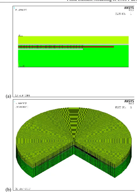
Figure II.2 The 2D axisymmetric ANSYS model of a RF-CMUT cell in (a)
an unmeshed 2D view and (b) a meshed 3/4 expansion showing the
equivalent 3D structure. ... 19
Figure II.3 The 2D axisymmetric ANSYS model of a RF-CMUT cell with
the propagating fluid coupled to the structural model in (a) an unmeshed 2D view and (b) a meshed 3/4 expansion showing the equivalent 3D structure.21
Figure II.4 The modelling of the volumes of the spatial period of an
RF-CMUT array composed of circular membranes arranged by (a) square tiling and (b) hexagonal tiling... 24
VI
Figure II.5 The 3D ANSYS model of the spatial period of RF-CMUT array
of circular cells arranged by (a) square tiling and (b) hexagonal tiling. The model includes the propagating fluid coupled to the structural model and the acoustic backing below the transducer device. ... 24
Figure II.6 The geometry modelled by (a) the axisymmetric model and (b)
the 3D model of the hexagonally tiled membranes. ... 25
Figure II.7 The first mode mechanical resonance frequency for the
RF-CMUT device described in Table II.1, computed by performing the modal analysis on the 3D model by varying the meshing elements size. The dashed line represents the result obtained by using the 2D axisymmetric model of the same device. ... 26
Figure II.8 The model complexity, described by the equation count, for
different mesh sizes applied to the 3D model of the RF-CMUT described in Table II.1. ... 27
Figure II.9 The first mechanical resonance frequency plotted against the
model total equation count. ... 27
Figure II.10 Comparison between the mechanical impedance curves
computed by varying the mesh size... 28
Figure II.11 Electrical impedance simulated (a) real part and (b) imaginary
part compared to the measured (c) real part and (d) imaginary part of the 1st
device. Simulations and measures were performed by varying the bias voltage. ... 29
Figure II.12 Electrical impedance simulated (a) real part and (b) imaginary
part compared to the measured (c) real part and (d) imaginary part of the 2nd
device. Simulations and measures were performed by varying the bias voltage. ... 30
Figure II.13 Comparison between (a) the simulated transmission transfer
function and (b) the measured impulse response for both the described devices. ... 31
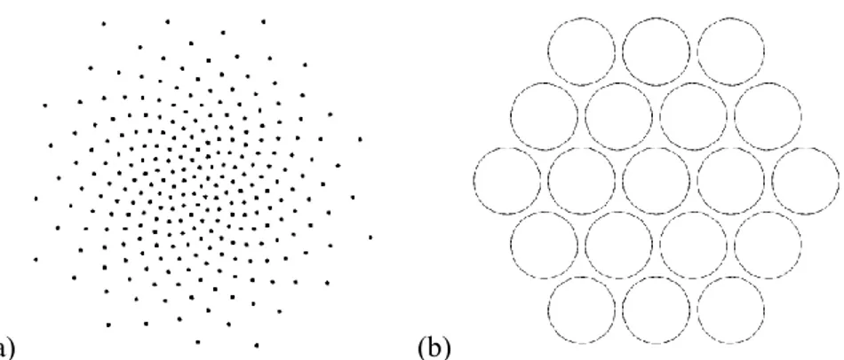
Figure II.14 The investigated 256-elements RF-CMUT sparse array with a
Fermat’s spiral-based layout. (a) The elements spatial arrangement and (b) the membrane pattern of each element. ... 32
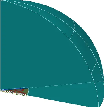
Figure II.15 The model of a 30° sector of the sparse array element modelled
in AutoCAD, (a) in an x-rays view and (b) in a side view. ... 33
Figure II.16 An x-rays view of the 30° sector of the sparse array element
modelled in AutoCAD. ... 33
Figure III.1 The modal shapes of the RF-CMUT membrane (a) at the first,
(b) at the second and (c) at the third resonant mode frequency, computed by the modal analysis (ANSYS). The colours represent the displacement along the direction normal to the radiating surface plane, ranging from the
minimum (blue) to the maximum (red). ... 37
Figure III.2 The mechanical impedance of the RF-CMUT device described
Figure III.3 The first axisymmetric mode frequency of the RF-CMUT
described in Table III.1 computed by varying the membrane radius, obtained by performing a modal analysis on the 2D axisymmetric FEM model
(ANSYS). ... 39
Figure III.4 The first axisymmetric mode frequency of the RF-CMUT
described in Table III.1 computed by varying the membrane thickness, obtained by performing a modal analysis on the 2D axisymmetric FEM model (ANSYS). ... 39
Figure III.5 The first axisymmetric mode frequency of the RF-CMUT
described in Table III.1 computed by varying the cavity height, obtained by performing a modal analysis on the 2D axisymmetric FEM model (ANSYS). ... 40
Figure III.6 Collapse voltage value computed by a finite element nonlinear
static analysis (ANSYS) by varying the membrane radius of the device described in Table III.1 from 20 μm to 50 μm. ... 43
Figure III.7 Collapse voltage value computed by a finite element nonlinear
static analysis (ANSYS) by varying the membrane thickness of the device described in Table III.1 from 1 μm to 2 μm. ... 43
Figure III.8 Collapse voltage value computed by a finite element nonlinear
static analysis (ANSYS) by varying the cavity height of the device described in Table III.1 from 0.1 μm to 0.3 μm. ... 44
Figure III.9 The membrane deflection profile computed by varying the bias
voltage Vdc = αVcoll, with α varying from α = 0.05 to α = 0.95. ... 44
Figure III.10 The membrane maximum displacement computed by varying
the bias voltage Vdc = αVcoll, with α varying from α = 0.05 to α = 0.95. ... 45
Figure III.11 The static capacitance value of the RF-CMUT cell described
in Table III.1, computed by ANSYS by varying the bias voltage Vdc = αVcoll,
with α varying from α = 0.05 to α = 0.95. ... 46
Figure III.12 The first mode resonance frequency fm0 computed by the
modal analysis (ANSYS), performed by varying the bias voltage Vdc =
αVcoll, with α varying from α = 0.05 to α = 0.95. ... 47
Figure III.13 The voltage across the electrodes, the membrane average
displacement and the pressure propagating in the fluid in the time domain, computed by a transient analysis (ANSYS). ... 50
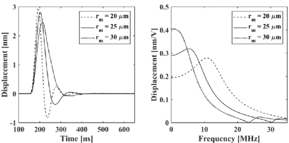
Figure III.14 The membrane average displacement in the time domain (left)
and in the frequency domain (right), in response to a broadband raised cosine voltage pulse, computed by varying the membrane radius. ... 52
Figure III.15 The membrane average displacement in the time domain (left)
and in the frequency domain (right), in response to a broadband raised cosine voltage pulse, computed by varying the membrane thickness. ... 52
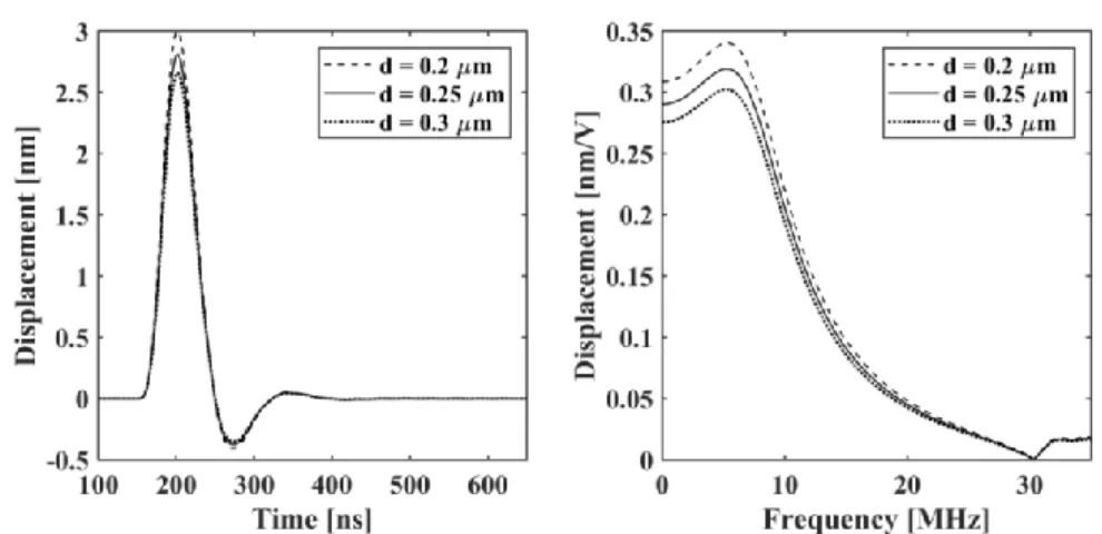
Figure III.16 The membrane average displacement in the time domain (left)
and in the frequency domain (right), in response to a broadband raised cosine voltage pulse, computed by varying the cavity height. ... 53
VIII
Figure III.17 The transmitted pressure in the time domain (left) and in the
frequency domain (right) computed by varying the membrane radius... 54
Figure III.18 The transmitted pressure in the time domain (left) and in the
frequency domain (right) computed by varying the membrane thickness. .. 54
Figure III.19 Normalized Transmission Transfer Function (TTF) computed
by varying the membrane radius. ... 55
Figure III.20 Normalized Transmission Transfer Function (TTF) computed
by varying the membrane thickness. ... 55
Figure III.21 The transmitted pressure in the time domain (left) and in the
frequency domain (right) computed by varying the cavity height. ... 56
Figure III.22 The voltage echo in the time domain (left) and in the
frequency domain (right) computed by varying the membrane radius... 57
Figure III.23 The voltage echo in the time domain (left) and in the
frequency domain (right) computed by varying the membrane thickness. .. 57
Figure III.24 The voltage echo in the time domain (left) and in the
frequency domain (right) computed by varying the cavity height. ... 58
Figure III.25 The membrane average displacement in the time domain (left)
and in the frequency domain (right), computed by varying the bias voltage. ... 59
Figure III.26 The transmitted pressure in the time domain (left) and in the
frequency domain (right) computed by varying the bias voltage. ... 59
Figure III.27 The voltage echo in the time domain (left) and in the
frequency domain (right) computed by varying the bias voltage. ... 60
Figure III.28 The TTF computed by varying the bias voltage in pulse-echo
behaviour simulation. ... 60
Figure III.29 The RTF computed by varying the bias voltage in pulse-echo
behaviour simulation. ... 61
Figure III.30 The membrane average displacement in the time domain (left)
and in the frequency domain (right), computed by varying the backing acoustic impedance. ... 63
Figure III.31 The transmitted pressure in the time domain (left) and in the
frequency domain (right) computed by varying the backing acoustic
impedance. ... 63
Figure III.32 Transmission Transfer Function (TTF) computed by varying
the backing acoustic impedance. ... 64
Figure III.33 Reception Transfer Function (RTF) computed by varying the
backing acoustic impedance. ... 64
Figure III.34 The voltage signal generated by the first echo received from
the load, in the time domain (left) and in the frequency domain (right), computed by varying the backing acoustic impedance. ... 65
Figure III.35 The voltage signal generated by the second echo received
from the load (first reverberation signal), in the time domain (left) and in the frequency domain (right), computed by varying the backing acoustic
Figure III.36 The reverberation level (RL), computed as the ratio between
the second and the first received voltage echoes, computed by varying the backing acoustic impedance. ... 66
Figure IV.1 Geometry of an arbitrary source observed from a generic point
P(r,θ,ϕ) ... 67
Figure IV.2 The directivity of a circular aperture a vibrating with a uniform
normal velocity, radiating pressure with ka = 10. The radiated pressure field is null for θ = 22.5° and θ = 44.5°. ... 69
Figure IV.3 The radiation pattern of a linear array of rectangular elements:
(a) the repetition of the array factor according to the elements spacing, (b) the element factor modulating the grating lobes, (c) the steered beam within the main lobe of the element directivity. ... 71
Figure IV.4 Contour plot of the z-component of the displacement, obtained
by a static analysis (ANSYS) performed by biasing the sparse array element with Vdc = 157 V. ... 73
Figure IV.5 Contour plot of the z-component of the displacement, obtained
by a static analysis (ANSYS) performed by biasing the sparse array element provided with the BCB backing layer with Vdc = 0.9 Vcoll. ... 73
Figure IV.6 Average transmitted pressure computed by harmonic analysis
(ANSYS) at f = 7 MHz. ... 74
Figure IV.7 Different frames showing the pressure wave traveling from the
transducer surface through the acoustic medium at f = 7 MHz. ... 75
Figure IV.8 Different frames showing the displacement along the z-axis (the
pressure wave propagation direction) at f = 7 MHz. ... 75
Figure IV.9 Acoustic radiation pattern obtained from the pressure computed
at a distance R = 500 μm from the radiating surface of the transducer. ... 76
Figure IV.10 Comparison between the array element beam pattern in the
case of clamped substrate with the beam pattern of the backed device. For this latter case, three different boundary conditions are applied to the outer edge of the element. ... 77
Figure IV.11 The simulated beam pattern (ANSYS) computed by assuming
the array element included in a continuous structure, to reproduce the
boundary conditions of the measured device. ... 78
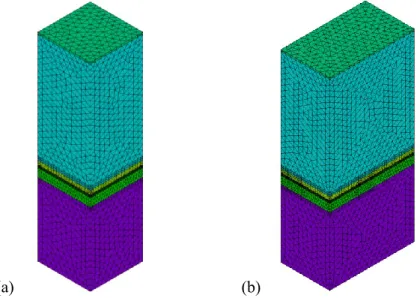
Figure V.1 3D FEM structural model of a circular piezoelectric unimorph,
meshed with (a) hexahedral elements and (b) tetrahedral elements. ... 81
Figure V.2 a) 2D axisymmetric structural model of a circular piezoelectric
unimorph and (b) the model 3D expansion. ... 82
Figure V.3 The structure of the proposed device in (a) an exploded view of
the array and (b) an assembled single cell section. ... 83
Figure V.4 2D axisymmetric FEM model of the complete transducer
flexural cell. The cell includes the steel front plate (grey), the piezoelectric layer (yellow), the epoxy rails (green), the brass back plate (orange) and the thin glue between the front plate and the piezoceramics (non-visible). ... 84
X
Figure V.5 Measurement setup for the evaluation of the average longitudinal
propagation velocity of the acoustic waves in a sample of concrete. ... 84
Figure V.6 The radius and thickness design curve for a steel plate resonating
at its first flexural mode at f0 = 110 kHz. ... 86
Figure V.7 The amplitude of the resonant device mechanical impedance,
computed by FEA on the structural model of the transducer by varying the thickness of the piezoelectric disk underlying the front plate. ... 87
Figure V.8 The amplitude of the resonant device mechanical impedance,
computed by FEA on the structural model of the transducer by varying the radius of the membrane. ... 88
Figure V.9 The amplitude of the resonant device mechanical impedance,
computed by FEA on the structural model of the transducer by varying the thickness of the membrane. ... 88
Figure V.10 The amplitude of the transducer RTF, computed by FEA by
varying the thickness of the piezoelectric disk underlying the front plate. .. 89
Figure V.11 The amplitude of the transducer RTF, computed by FEA by
varying the thickness of the epoxy layer patterned with the cavities, clamped at the lower edge... 90
Figure V.12 The amplitude of the displacement along the normal direction
(y-axis) computed at the frequency of the maximum RTF amplitude by varying the rail layer thickness. ... 91
Figure V.13 An example of flexural deformation of the membrane
supported by the rails moving (a) upwards and (b) downwards in time. The frames were taken from a time-harmonic animation of the device with tr = 1.6 mm at the frequency fMAX = 186 kHz, where the RTF is maximum. 91
Figure V.14 The amplitude of the transducer RTF, computed by FEA by
varying the thickness of the brass back plate. ... 93
Figure V.15 The amplitude of the transducer RTF, computed by FEA, on
List of tables
Table II.1 Geometrical parameters of the modelled RF-CMUT device ... 25 Table II.2 Geometrical parameters of the simulated and measured devices 29 Table II.3 Geometrical parameters of the RF-CMUT cells composing the
sparse array element ... 32
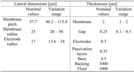
Table III.1 Geometrical parameters of the simulated device and their
variation range ... 36
Table III.2 Material parameters used in the simulations ... 36 Table III.3 Measured material properties of the backing compounds. ... 62 Table IV.1 Material parameters used in the sparse array element simulation.
... 72
Table V.1 Material properties of the structural layers used for the
simulation. ... 85
Table V.2 Material constants used for the PZT5-H material. ... 85 Table V.3 Variation range of the geometrical parameters of the FEM model.
Abstract
This work describes the finite element modelling and characterization of ultrasonic flextensional transducer arrays. Flexural acoustic transducers can be piezoelectrically actuated plates or capacitive devices based on the electrostatic attraction between a moving electrode and a substrate. Due to the limited miniaturization allowed by the piezoceramic fabrication process, piezoelectric flexural devices based on bulk ceramics are able to work in the low-frequency ultrasonic range. Capacitive flexural devices, instead, can take advantage of the Silicon micromachining techniques to be fabricated to reach higher frequencies.
Capacitive Micromachined Ultrasonic Transducers (CMUTs) are MEMS devices consisting of miniaturized metallized membranes, forced into flexural vibration by an electric signal during transmission, and vice versa generating a voltage signal when actuated by an incident acoustic signal. Due to their low acoustic impedance, CMUT arrays have given excellent results in ultrasound imaging applications.
The most recent frontier of ultrasound imaging is real-time volumetric imaging. 3D images have been originally obtained by means of linear phased arrays mechanically titled along the elevation plane. More complex structures like 2D arrays allow electronic beam steering and dynamic focusing in both azimuthal and elevation planes, thus achieving better performance. In order to increase the achievable frame rate, though, part of the front-end transceive and beamforming operations must be performed in probe. Therefore, 2D arrays should be small-sized and easily interfaced with the front end. Nevertheless, 2D arrays with good radiation characteristics require wide apertures with a small pitch between elements, therefore a great number of elements and many channels to wire and control individually. To overcome these issues, much attention is being focused on the design of sparse arrays, which try to achieve comparable performance by counting a lower element number.
For the design of optimized CMUT devices, accurate modeling is mandatory: the propagation of the acoustic wave produced by a source made of multiple vibrating membranes radiating into a fluid-like medium cannot be fully described by analytical models, thus CMUT devices must be simulated by Finite Elements Models (FEM). In this work, a simplified model of a wide
XIV
aperture multicell CMUT device was used to develop a tool to support the design process. The model was used to investigate the design parameters variation effect on the static and dynamic performance of CMUT arrays composed of circular cells. The collapse voltage, the membrane deflection profile and the static capacitance of Reverse-Fabricated CMUT devices (RF-CMUTs) were computed by varying the membrane radius and thickness and the cavity height. Since devices fabricated by the Reverse Fabrication Process are built from top to bottom, the Silicon Nitride base can be made very thin, and the devices can be backed by arbitrarily designed backing layers. The backing material effect on the pulse-echo behavior of immersed CMUT devices was investigated, and the reverberation phenomenon reduction was observed by matching the backing material acoustic impedance to the acoustic impedance of the propagating medium.
In order to investigate the performance of a sparse CMUT array, a 3D FEM model is needed, since there is no axial symmetry in a sparse array layout. For this reason, a full model of a reverse CMUT cell was implemented, tested and experimentally validated. Due to the long simulation time required by the FE analysis of a finite transducer element, a mesh optimization study was carried out on a simpler structure, i.e. an infinite transducer. The results of this optimization process were used to mesh a CAD-imported model of a sparse array element.
The studied array element is part of a multi-chip module (MCM) comprising a CMUT array based on a density tapered Fermat’s spiral and an analog front end (AFE) ASIC wafer-bonded to the transducer array by means of a Benzocyclobutene (BCB) layer. The 10-mm array is designed for broadband operation around 7 MHz in immersion operation, and is made by 256 1.0λ-wide elements consisting of 19 hexagonally tiled circular cells.The proposed model was used to perform a harmonic analysis in ANSYS, in order to compute the element factor that modulates the array radiated pressure field. The study of the array element directivity is important to assess the beam steering capabilities of the device.The beam pattern was computed by varying the mechanical boundary conditions applied to the array element, in order to investigate the effects of an acoustic isolation of the array element, achievable by performing trenches in the BCB layer or in both the BCB and the structural nitride. The results obtained for the device included in an infinitely extended structure are in good agreement with the measurement performed on the probe head prototype featuring the MCM, though some differences in the main lobe and side lobe level exist, probably due to the incorrect compensation for the hydrophone directivity applied.
The FEM model of the wide aperture multicell CMUT was used as a basis to model a flextensional array of circular membranes actuated by piezoelectric disks, housed inside the cavity and glued to the rear of the membrane. The transducer array was designed for broadband reception operation in concrete-coupled condition, in order to perform efficient acoustic emission
measurements for the monitoring of concrete structures. The piezoelectric flextensional array design process was based on the computation of the device reception transfer function, obtained in concrete-coupled conditions by varying the geometrical parameters of the elastic plate, of the structural layer and of the backing. The resulting device has a 200 kHz wide -6 dB reception sensitivity bandwidth around the center frequency of 112 kHz, thus is suitable for acoustic emission techniques applied to concrete structures.
Introduction
This work is a study on ultrasonic acoustic transducers based on plates moving by flexural vibration. The applications considered are ultrasound imaging and acoustic emission techniques for the monitoring of concrete structures.
In this kind of devices, the generation and reception of acoustic waves is obtained by the vibration of membranes with fixed rim, which bend and extend along the direction normal to their surface. Ultrasonic transducers based on flexural plates are devices able to convert energy from the electrical to the mechanical domain, and vice versa. The operating principle can be piezoelectric or capacitive. In the case of piezoelectric flextensional transducers, the flexural vibration and normal extension of an elastic membrane is obtained by exciting a piezoelectric element coupled to a bending plate. The deformation of the piezoceramic bends the membrane causing the flexural deformation that originates the transmission of an acoustic wave. In the case of capacitive transducers, a hollow cavity is obtained inside an elastic structure, and two electrodes are placed on top and at the bottom of the gap. By applying a static voltage across the electrodes, the electrostatic force causes the bending of the top plate towards the substrate. Providing an alternate voltage signal makes the suspended membrane move by flexural vibration, generating an acoustic wave. The main characteristics of flextensional devices is that their mechanical impedance is much lower than the mechanical impedance of thickness mode piezoelectric transducers, which makes them particularly suitable for broadband operation when coupled to low-to-medium acoustic impedance propagating media.
The broadband sensitivity of flexural membranes is centred around the frequency of the first resonant mode of the membrane. The first resonance frequency is inversely proportional to the square of the membrane size, therefore the maximum frequency of operation achievable by an ultrasonic device is determined by the miniaturization level allowed by the fabrication process. The techniques for the fabrication of piezoelectric bulk ceramic plates and disks do not allow miniaturization below the mm-scale. For this reason, piezoelectric flexural devices based on bulk piezoceramics can be used for sensing and non destructive testing applications, which require frequencies of
XVIII
operation below the MHz. Ultrasound imaging, instead, is performed at frequencies above 1 MHz an up to 20 MHz, therefore flexural devices for imaging must have apertures of tens-to-hundreds of microns. Piezoelectric devices with dimensions in the sub-mm scale can only be obtained by film deposition. On the contrary, capacitive transducers can be fabricated as MEMS devices by taking advantage of the well-known Silicon micromachining techniques, and therefore can work at high frequency with a reduced technological effort. These devices are known as CMUTs – Capacitive Micromachined Ultrasonic Transducers. CMUTs can reach high performance in the medical ultrasound imaging application. In particular, the CMOS-compatible fabrication technique of CMUTs makes these devices very appealing for critical imaging applications, such as real-time volumetric imaging. In fact, in order to perform successfully a high frame-rate volumetric imaging, the front-end electronics should be placed in probe; therefore, the transducer array must be small-sized and directly coupled to the transceiver electronic and the beamforming circuits.
The investigation of the propagative behaviour of such ultrasonic devices involves a coupled-field analysis that requires multiphysical PDEs solution, unless strong simplifications are assumed. A reliable prediction of the devices electroacoustic behaviour, which is necessary for an accurate application-specific design, requires simulation by finite element analysis. In this work an ANSYS FEM model for the simulation of ultrasonic transducer arrays is developed. The FEM model of CMUT devices is used to investigate the performance of dense and sparse 2D arrays for medical imaging. Wide aperture multicell devices are simulated by means of a 2D axisymmetric model, and a sparse array element is simulated by a 3D model with finite dimensions. FEA is also used to support the design of a piezoelectric device for acoustic emission techniques for the structural monitoring of concrete structures.
Chapter I introduces CMUT devices for ultrasound imaging, describing the most common types of probes and focusing on a new 2D sparse array of Reverse-Fabricated CMUTs based on a Fermat’s spiral pattern.
Chapter II thoroughly describes the developed FEM models for the simulation of multicell CMUTs, such as 2D dense arrays or wide aperture single element transducers, and for the simulation of the directivity pattern of a sparse array element.
The effect of the variation of the structural dimensions and of the bias voltage on the static and dynamic transmission and reception performance of immersed CMUT devices is analysed in Chapter III, thus showing how FEM can support the design process by leading to the CMUT device optimization.
Chapter IV is dedicated to the performance analysis of the 2D spiral array element, whose one-way beam pattern is compared to the measured directivity of the fabricated prototype.
Finally, the design of a flextensional transducer, based on piezoelectric disks activating the flexural vibration of an array of membranes, is carried out in Chapter V. Such piezoelectric flextensional array is optimized for the application to acoustic emission techniques applied to concrete structures, for the structural health monitoring.
Chapter I
CMUT arrays for ultrasound
imaging
I.1 Transducers for medical ultrasound imaging
Ultrasound (US) imaging is the preferred technique for the investigation of human body tissues, such as organs, muscles, tendons and vessels. In fact, US imaging offers several advantages over other available imaging techniques: it is completely harmless and non-invasive, provides real-time images and is cost-effective. Images of anatomic structures are obtained by transmitting and receiving ultrasonic acoustic waves propagating through the human body, by means of an electroacoustic transducer device. The fabrication technology of transducer arrays for ultrasound imaging based on piezoelectric materials is nowadays very mature and therefore hardly improvable. During the last two decades, excellent results were obtained by new MEMS devices, fabricated by silicon micromachining technology and based on the electrostatic cell working principle. These devices are known as CMUTs, which stands for Capacitive Micromachined Ultrasonic Transducers. Transducer arrays fabricated by CMUT technology have reached top-level performance.
The use of arrays instead of solid apertures for medical imaging can be easily justified by the numerous advantages arrays grant with respect to single-crystal transducers [1], [2]. For instance, using multiple active elements allows for electronic beam steering and focusing. Besides, the use of arrays enables the adjustment of the lateral resolution and the beam shaping by the electronic aperture apodization, which means that the active aperture can be changed dynamically by exciting only a part of the available array elements. Moreover, a dynamic focusing can be obtained in receive mode, so that the highest resolution achievable can be maintained through the entire scan depth. It should also be noticed that all of these features can be obtained without mechanically tilting the probe, therefore reducing the needs for mechanical maintenance.
Chapter I
2
I.1.1 1D arrays
1D arrays, such as linear arrays, curvilinear arrays and phased arrays, are made by several elements arranged along a line and controlled independently from one another. Let us suppose the elements are arranged along the
x-direction on the xy plane, and the propagation of ultrasonic waves takes
place along the z-direction. These kinds of transducer arrays generate images of planar sections of the human body, and allow dynamic focusing in the azimuthal (xz) plane. The focus in the elevation plane (yz) is fixed by an acoustic lens.
Linear arrays are usually made by up to 256 elements, but only a small number of elements are excited at the same time. The resulting image has a rectangular shape, with a constant density of scan lines.
Convex arrays, also called curvilinear arrays, are essentially linear arrays arranged on a curved convex structure. Due to the natural divergence of such shape, the sequential excitement of a small number of adjacent elements allows the scanning of a wider sector of the azimuthal plane, hence returning an annular sector of the scanned plane with a line density decreasing by increasing the depth.
Phased arrays count up to 128 elements, as they are designed to have a smaller footprint in order to investigate parts of the body with small access areas. As for linear arrays, the number of elements excited at the same time can be varied, but the fired elements are always centred at the centre of the array. Moreover, by exciting the elements with a different amplitude (electronic aperture apodization), the active area of the transducer can be electronically reduced to have a wider main lobe of the radiation pattern, or the array can be excited by signals whose amplitude is modulated by a Hanning window, in order to reduce the side lobe level. By providing phased input signals, instead, the transmitted beam can be steered in order to focus at different depths on the propagation direction, on a wide angular range of the azimuthal plane. In this way, a wider part of the body in front of the transducer surface can be investigated by a small aperture, obtaining a trapezoidal shaped image of the investigated area. This feature is particularly useful for cardiac imaging applications, where the probe head must fit in between the ribs in order to reach the heart without any shading caused by the bones. Also in this case, the line density decreases at the bottom of the image.
I.1.2 2D arrays
2D arrays are made by elements arranged along rows and columns. By controlling the array elements individually along both directions, the input signals can be tuned in order to have the beam steered and focused at different depths on the elevation plane as well as on the azimuthal plane, thus granting much more flexibility with respect to 1D arrays. The dynamic focusing in an
arbitrary point of the half space facing the transducer made available by 2D arrays has moved increasing attention towards the imaging of volumes. The steep improvement in the computational power of modern architecture also fostered the development of volumetric imaging performed in real-time, in order to observe moving volumes with an acceptable frame rate. This feature is particularly interesting for the diagnosis of cardiac diseases.
With respect to traditional probes for volumetric US imaging, the capability of 2D arrays to steer the beam electronically in both azimuthal and elevation direction eliminates the need for mechanical rotation and tilting of the probe, with a consequent increase of the achievable frame-rate. In fact, volumetric imaging has been traditionally performed by means of mechanical 3D probes: such probes are based on 1D linear or convex arrays, moved under computer control or by freehand translation to collect the 2D frames used to render the volume of the investigated region. The rotation and tiling of the conventional 1D transducer array is performed either by an external fixture (rather bulky and heavy) or by an in-probe integrated positioning system [3], [4]. Although this technique is effective for the rendering of the observed volume, the mechanical scan is inevitably too slow to allow real-time imaging of moving volumes. Moreover, it is strongly subject to errors and uncertainty, due to the necessity of position-sensing devices and tracking systems. 2D arrays do not require this increased complexity, as they rely on electronic scanning, which is undoubtedly faster. The first attempts at volumetric imaging by means of 2D arrays date back to 1991, when a preliminary real-time 3D scan with 8 frames/s was demonstrated by means of a 289-elements piezoelectric transducer array [5], [6]. Developing fully sampled matrix arrays, though, introduced new issues to deal with. Due to the spatial repetition of elements across the array surface, grating lobes can arise in the radiation pattern. Grating lobes cause dispersion of the radiated energy, and are responsible for the formation of artefacts on the ultrasound image. In order to avoid the formation of grating lobes in the directivity pattern of the radiated pressure field, the distance between adjacent cells (pitch) should be less than half wavelength. On the other side, large apertures are required for a good lateral resolution. Therefore, having a wide aperture and small elements means dealing with a very high number of elements, and each of them must be controlled individually. The consequences are a high difficulty in the channel wiring, a great complexity of the front-end electronics, a strong power dissipation and, finally, a high cost. For this reason, the first 3D scan system based on 2D transducers, proposed in 2002 by Philips, reduced the data coming from about 3000 acoustic elements to just 128 signals according to the method described in [7], which could then be processed by a conventional ultrasound system. Soon after, a fully sampled 2D array made by CMUT technology was proposed, though the first volumetric images obtained by means of a CMUT probe were produced by a small 16x16 elements sub-array [8]. Even now, the only way to use fully-sampled arrays to perform real-time
Chapter I
4
volumetric imaging is to scale down the channel number to a maximum of 256 [9], [10].
One possible solution to reduce the number of channels to be wired and connected to the external ultrasound system is to implement μ-beamforming techniques for the beam formation and received signal processing [11], [12]. The beamformer is the system in charge of controlling the ultrasonic beam characteristic in transmission and reception. The transmit beamformer generates the delay pattern of the input signals, in order to steer and focus the beam. The receive beamformer delays the signals received from different depths and sums the realigned signals, in order to provide the data for the image reconstruction. The beamforming in reception is usually performed according to delay-and-sum (DAS) algorithms, even though non-linear algorithm such as the delay-multiply-and-sum (DMAS) have also been proposed for a higher dynamic range in B-mode images [13]. The beamforming can be performed digitally [14] or analogically [15]. Analog beamforming is not suitable for 2D arrays, as it does not allow dynamic focusing and requires a considerable area to include all the needed components. Digital beamforming, nonetheless, also requires space on the ASIC for the analog-to-digital converters (one for each element), and is therefore not suitable for high element counts. In the case of a high element number, the μ-beamforming is a valid solution to reduce the number of cables connected to the external imaging system. The μ-beamforming is a two-steps beamforming technique, where the transducer array is divided into sub-apertures. The echo signals from the elements of each sub-aperture are processed by an in-probe ASIC, which performs a preliminary realignment of the echoes and returns one output signal for each sub-aperture into which the array is divided. In this way, only one cable per sub-aperture is routed to the main beamformer in the external imaging system, which combines the signals pre-processed by the μ-beamformers into one final output signal used for the image reconstruction [16]. This method is currently used in commercial real-time 3D imaging systems.
In order to overcome the issues related to the connection of a high element number, much attention is also being focused on the design of sparse arrays, which try to maintain acceptable performance while counting a lower element number. Lessening the element count also increases the achievable frame rate of volumetric imaging, since it reduces the amount of data that must be processed. For this reason, sparse arrays have become even more appealing with the increasing interest for volumetric imaging. Removing elements from the array, though, intrinsically lowers the array sensitivity, and at the same time degrades the acoustic beam pattern, as the energy missing from the main lobe reappears in the form of grating lobes or by increasing the side lobe level. The issues related to sparse array design were already faced in the early 1990s [17]–[19], and new methods are still under investigation [20]–[24]. Grating lobes can be avoided by breaking the spatial periodicity of the remaining
active elements, but improving the sparse array performance over a wide range of steering angles requires a strong effort in the design optimization. Recently, good results were obtained by arranging the elements outside of the rows and columns of a grid, by following a spiral pattern [25]. In particular, a method for the design of a sparse array realized by arranging cell clusters according to a Fermat’s spiral pattern has been proposed [26]. Simulation results encourage the study of this particular array topology in order to obtain good performance with a limited number of active elements. The improvement in 2D array design are particularly important for the outcome in real-time volumetric cardiac imaging, which is undoubtedly the critical application for ultrasound imaging.
I.2 History and state-of-art of CMUTs
I.2.1 CMUT devices
Capacitive Micromachined Ultrasonic Transducers (CMUTs) are MEMS devices consisting of metallized Silicon membranes suspended over a cavity, with the outer edge clamped onto a conductive substrate. The membranes are set into flexural vibration by an electric signal during transmission, and vice versa generate a voltage signal when actuated by an incident acoustic signal. A multitude of electrostatic cells represents a CMUT array.
CMUTs were firstly developed in the mid-1990s [27], mainly pushed by the idea of obtaining high-frequency ultrasonic transducers for air-coupled operations. In fact, technological issues do not allow the use of piezoelectric devices at high frequencies in air. The acoustic impedance mismatch between the piezoceramic and the air requires the interposition of matching layers between the two materials; though, finding low-loss materials with the needed acoustic impedance is not a simple task. Moreover, the thicknesses required for operation in the MHz range are unachievable for such materials. On the contrary, CMUTs have an intrinsically low mechanical impedance, so they have been soon recognized as suited for coupled operation. Efficient air-coupled transmission was soon demonstrated [28], [29], and shortly followed by the demonstration of broadband water-coupled transmission [30]–[32]. As the first results proved CMUTs could compete with piezoelectric devices for immersion operation [33], the first CMUT-based devices for medical ultrasound imaging appeared: fully functional 1D linear [34] and phased arrays [35], 2D dense arrays [36] and annular arrays [37] were fabricated and characterized. Soon after, the first ultrasound images obtained by means of CMUT devices were demonstrated [38]–[41]. Since then, several other CMUT arrays for imaging applications were proposed [42], [43] before Hitachi Medical Corp. came out with the first commercial CMUT probe in 2009. Later, research has moved great steps towards the optimization of CMUT arrays for high-performance ultrasound imaging [44]–[48]. Finally,
Chapter I
6
during the last years, CMUT technology became consolidated and is currently transforming from a research topic to a commercial reality.
I.2.2 CMUT fabrication techniques
CMUT arrays are fabricated by surface micromachining techniques [49]. The traditional approach to CMUT fabrication starts from a Silicon wafer, where a sacrificial layer is deposited and covered by the Silicon Nitride membrane layer by Low-Pressure Chemical Vapor Deposition (LPCVD). In the first reported technique, the sacrificial layer was an oxide layer, removed by a selective wet etching process through vias created in the membrane. In this way, a vibrating freestanding structure is created [50], [51]. Figure I.1 describes the steps for the fabrication of CMUT devices by the classic sacrificial-release technique.
(a) (d)
(b) (e)
(c) (f)
Figure I.1 An example of a traditional sacrificial-release fabrication process,
as described in [50]. The frames show: (a) the starting Silicon wafer, (b) the Silicon oxide growth, (c) the LPCVD Silicon Nitride deposition, (d) the Au metallization deposition, (e) the membrane etching, (d) the sacrificial layer etching.
In the early years of CMUT technology development, also examples of CMUT-on-CMOS were reported [52]. The deposition technology quickly switched to Plasma-Enhanced Chemical Vapor Deposition (PECVD), in order to keep the temperature below 400°C, and the use of Chromium as sacrificial layer was described [35]. Since the classical fabrication technique requires to make vias through the membrane to empty the cavity, which can affect the acoustic performance of the device, different techniques for the transducer fabrication were investigated. One example is the transducer assembly by wafer bonding [53]. Another solution was proposed by Roma Tre University [54], [55], where a technique named Reverse Fabrication Process was developed. The steps for the fabrication of CMUTs by reverse technology are described in Figure I.2. By reverse fabrication, CMUTs are built from top to bottom, starting from a Silicon wafer already covered by a layer of LPCVD
Silicon Nitride. The top electrode is realized by Aluminum evaporation, and then covered by a passivation Silicon Nitride layer, deposited by PECVD. On top of the Nitride layer, the sacrificial layer of Chromium is deposited. Chromium is then removed from the areas that must be filled with another deposition of the structural Silicon Nitride, in order to shape the cell. Afterwards, the second electrode and the last Silicon Nitride layer are deposited. Finally, vias are made through the structural layer to reach the remaining Chromium, which is etched by a selective wet etch process to create the cavity. In this way, the holes are drilled into the bottom layers of the device, so that they do not affect the acoustic behavior of the membranes. An arbitrarily shaped backing layer made of a sound-absorbing material, such as epoxy resin, can be attached to the back surface of the CMUT array, in order to provide mechanical support and also improve the device performance by absorbing the incoming pressure signals. At this point, the device can be flipped upside down, and the silicon wafer is etched up until the LPCVD Silicon Nitride, thus releasing the membrane.
(a) (f)
(b) (g)
(c) (h)
(d) (i)
(e) (j)
Figure I.2 The steps for the fabrication of a CMUT device by reverse
fabrication process: (a) LPCVD SiN deposition, (b) top Al metallization deposition by evaporation, (c) passivation by PECVD SiN, (d) Chromium sacrificial layer deposition, (e) passivation by PECVD SiN, (f) bottom Al metallization deposition, (g) passivation and etching of the Nitride, (h) sacrificial layer etching, (i) base PECVD SiN deposition. Legend in (j). Images from [44].
Chapter I
8
I.2.3 CMUTs for the next generation of US imaging
After the development of fully functional CMUT based probes for ultrasound imaging, the technology was pushed forward by developing different kinds of CMUT-based probes for advanced applications. For example, side-looking catheters [56], for intravascular guidance and navigation, and forward-looking catheters [57], for intravascular therapy delivery and lesion assessment, were proposed and demonstrated to be feasible. The first in-vivo intravascular ultrasound image obtained with a CMUT array was obtained in 2012 [58]. Much more recently, an example of intravascular array for volumetric imaging in intracardiac echography was also proposed [59], in the view of a next generation of high-performing devices enabling improvements in life-saving technologies.
Some recent developments also concern the optimization of high-frequency CMUT arrays [60] and criss-cross arrays for biplane imaging [61].
For what concerns classical ultrasound imaging, the next frontier is high frame rate volumetric imaging, especially interesting for cardiac investigation. As previously outlined, volumetric imaging can be performed by 2D arrays, but a high frame rate can only be achieved by reducing the element count, hence by using sparse arrays. For this reason, there is currently a great interest in the development of 2D sparse arrays for fast, real-time 3D imaging. It should also be noticed that, by means of one single probe, whole-body imaging can be performed, since the wide bandwidth of CMUTs allows working at different frequencies and the aperture can be dynamically modified to suit the desired application.
Furthermore, CMUT devices can be more easily interfaced to the CMOS in-probe electronics with respect to traditional piezoelectric transducers. The feasibility of coupling the transducer array and the front-end ASIC (CMUT-on-ASIC) by flip-chip bonding techniques was investigated [62]–[64], and the coupling was successfully obtained for some of the available channels. The scope is the realization of integrated modules for miniaturized, low-weight, low-cost and energy efficient portable imaging systems. The peculiarity of these systems is that the transmit and receive beamforming is performed entirely by the ASIC device coupled to the CMUT array, and the data is processed in-probe. This will allow the development of all-in-one portable devices for point-of-care ultrasound, that can perform ultrasound imaging by simply connecting to a mobile device, such as a smartphone or a tablet, and can also send the data in the cloud to be shared. An example of such device was recently announced by Butterfly Network, Inc.
I.3 A Reverse-Fabricated 2D CMUT spiral array
The reasons behind the increasing attention towards sparse array configurations were introduced in Section I.1.2. Various random and
deterministic layouts of sparse arrays have been studied since the early 1990s. One deterministic pattern that prevents a periodicity in the spatial sampling of elements is the spiral pattern. Among all different spiral patterns, the Fermat’s spiral pattern for the arrangement of transducer array elements was considered in [65]. In a N-elements Fermat’s spiral based array, the position of the n-th element in polar coordinates is given by the couple
n n (I.1) 1 n n a N r R (I.2)
where α is the divergence angle, which determines the number of branches of the spiral, and Ra is the aperture radius.
The configuration obtained by using a divergence angle α equal to the golden angle
5 1
(I.3)
is also known as the “sunflower” pattern. The main characteristic of this pattern is that the spatial density of the elements is kept constant but there are no elements with the same angular position, hence any kind of spatial periodicity is prevented. For this reason, this particular spiral pattern was investigated for the design of a sparse CMUT array [66]. Spatial density tapering according to a Blackman tapering function was also introduced to reduce the side lobes level without introducing electronic apodization. Fabricating non-gridded array configurations with the fabrication approach used for piezoelectric transducers is particularly complicated. The fabrication of CMUT devices is much more suitable to the construction of these non-periodic structures. Reverse fabrication technology, in particular, has the advantage of allowing easy access to the connection pads, placed on the back of the device.
For this reason, a RF-CMUT spiral array was realized to be inserted in a Multi-Chip Module (MCM) comprising the transducer array and an ASIC, interconnected by means of a flip-chip bonding technique, according to the procedure described in [64], [67]. The RF-CMUT spiral array is designed for broadband operation in immersion around 7 MHz, with a two-way -6 dB fractional bandwidth of 100%. The array elements are 1.0λ wide (220 μm-wide aperture), arranged according to a sunflower pattern on a 10-mm quasi-circular area. Figure I.3 shows (a) the 6” wafer of the MEMS dice and (b) a close-up on the array die before the packaging operation.
Each element has a hexagonal shape and features 19 circular CMUT cells packed by hexagonal tiling with a centre-to-centre distance of 53 μm. Figure I.4 shows an optical microscopy view of (a) one array element and of (b) the CMUT spiral array.
Chapter I
10
(a) (b)
Figure I.3 RF-CMUT spiral array (a) dice on 6" wafer and (b) single die.
(a) (b)
Figure I.4 Optical microscopy view of (a) one 19-cells 1.0λ-wide hexagonal
element and (b) the RF-CMUT spiral array.
Figure I.5 Probe head prototype including the multi-chip module comprising
the RF-CMUT spiral array transducer flip-chip bonded to the analog front-end ASIC by means of an acoustically optimized integration technique.
The ASIC is a 256-channel analog front end (AFE), featuring unipolar pulsers and low-noise amplifier for the transceive operation, together with a programmable transmit beamformer. The channel pads layout was specifically optimized for the interface with the spiral transducer array. Figure I.5 shows a probe head prototype mounting the flip-chip bonded MCM.
Chapter II
Finite Element Modelling of
CMUT devices
II.1 The need for Finite Element Analysis in the study of CMUTs
The earlier models for the simulation of CMUT cells were based on the assumption of piston-like displacement of the membrane (uniform displacement along one axis, normal to the transducer surface), leading to the acoustic behaviour of a piston radiator and the electrical behaviour of a moving parallel plate capacitor. This theory is easily described by 1D models, usually linearized around a bias point, and since the early days of CMUT simulation transposed in a lumped parameter equivalent circuit [31], [50], [68]. Equivalent circuit models, featuring standard electrical components that represent mechanical, acoustic and electrical elements, allow the use of electrical network analysis to predict easily the behaviour of a complex vibrating system. Lumped parameters circuit always involve the presence of a transformer, which represents the energy conversion from the electrical domain to the mechanical domain and vice versa [69]. During the years, this kind of models have been expanded and improved in order to include the effects of other parameters, such as the electrode size [70], the atmospheric pressure [71], the air in the cavity (if present) [72], the interaction with nearby membranes [73] and some of the higher order modes [74].Another approach for the time-domain simulation of the nonlinear behaviour of CMUTs relies on the numerical solution of the simplified differential equations that describe the multiphysical system. These nonlinear models take into account the intrinsic nonlinearities of the electromechanical coupling (the electrostatic force depends on the square of the applied voltage, as will be explained in Section III.3), thus allowing the simulation of the effect of large signals applied across the electrodes. Nonlinearities are also figuring in equivalent circuit models in form of controlled sources [75].
Even if these models give accurate results around the first resonance frequency of the membrane, they fail in simulating the high frequency
Chapter II
14
behaviour of the transducer, where higher order modes intervene and determine a variation of the transmitted pressure. An analytical method for the simulation of higher order modes based on the mode superposition analysis was proposed in [76], but gives accurate results only after extracting the system parameters from measurements.
Consequently, the only reliable method for the time-domain simulation of the behaviour of CMUT devices that takes into account the acoustic fluid loading, the electromechanical coupling, the transducer non-linearity, the higher order resonant modes, the membranes cross-talk and the diffraction phenomenon is the Finite Element Method (FEM). Though very time consuming and computationally expensive, the Finite Element Analysis (FEA) is still the most complete tool for the accurate design of acoustic transducers.
By taking advantage of a circular CMUT cell rotational symmetry, a simple and light 2D axisymmetric FEM model of a CMUT cell was firstly presented in [77]. Originally, this model was used for the computation of the electromechanical coupling coefficient in conventional polarization [78] and in collapse-snapback regime [79], and then for the computation of the device electrical impedance in vacuum [80]. The axisymmetric FEM model was improved with the possibility to simulate the device propagative behaviour in [81], where the modelling of a fluid medium infinitely extended in the lateral directions by means of a cylindrical waveguide of fluid coupled to the transducer structural model was introduced. This acoustic coupling FEM model was then extensively used for the evaluation of the transmitted pressure in conventional operation and collapse-snapback operation [82], [83], and allowed the study of an impedance-matched backing effect on the CMUT arrays performance [82], [84]. 3D FEM models were also proposed for the simulation of different membrane geometries [85] and for the study of the cross-talk between near membranes [43]. These more accurate models were key-enablers for the design of high-performance CMUT dense arrays [42], [44], [86].
FEM simulation is the only simulation technique that can predict accurately also the performance of sparse arrays, where the directivity function of a small radiating element depends on the solution of the diffraction integral, and is strongly influenced by the acoustic interaction of a small number of membranes close to each other. The implementation of a FEM model of a dense array was then considered a preliminary step for the realization of a more complex model of a Fermat’s spiral-based sparse array element.
The next section introduces the infinite transducer model, a simplified model that represents a wide aperture device made by closely packed, regularly spaced circular membranes, implemented in ANSYS (ANSYS Inc, Canonsburg, PA) by means of a 2D axisymmetric model and a 3D model. The infinite transducer model was used to compute the mesh size that was applied
in the meshing of the Fermat’s spiral sparse array element described in the last section of this chapter.
II.2 The infinite transducer model
Large, regular arrays, where a high number of membranes are arranged in a grid-like fashion and are all operated in parallel for maximum output pressure, allow the exploitation of symmetry for the implementation of reduced-order FEM models. Such lighter models have the invaluable advantage of requiring shorter times for the simulation of time-domain signals propagation, without losing results accuracy.
By assuming the array lateral extension is large enough compared to the signal wavelength at the operating frequency, we can consider the transducer as if it were an infinite source radiating plane waves into the half space. Symmetry boundary conditions applied at the edge of one single cell create the model of an unbounded transducer, which extends infinitely on a plane orthogonal to the wave propagation direction. In such situation, the membranes composing the array would be all vibrating in phase, in a fluid of real acoustic impedance. For this reason, the assumption of wide aperture allows to simulate one single cell radiating plane waves, and then extend the results to the entire dense array made of several identical cells.
In order to support plane wave propagation, the semi-space of fluid can be represented by a cylindrical rigid-walled acoustic waveguide having a cut-off frequency higher than the maximum frequency involved in the analysis, in order to avoid the excitation of guided propagation modes. In fact, below the cut-off frequency of the first nonplanar mode of a rigid-walled waveguide with circular section, only plane waves can propagate, as if the signal were radiated in an infinitely extended medium [87]. The diffraction phenomenon gives an upper frequency limitation to the validity of such model. By increasing the frequency, the plane waves travel along the propagation direction with an increased angle θ with respect to the longitudinal axis [1]. At high frequencies, angled plane waves are reflected by the lateral rigid walls of the fluid waveguide, originating stationary waves that invalidate the model results.
As a consequence of this consideration, a dense array of regularly spaced identical cells can be modelled, in a reasonably wide frequency range around the first resonance mode of the device, by a single CMUT cell replicated along both lateral directions, radiating in a cylindrical column of fluid. The fluid waveguide radius matches half the centre-to-centre distance of the membranes, thus taking into account the spatial periodicity of the array.
If the cell has a circular geometry, the first resonance mode around which the sensitivity bandwidth in centred is an axisymmetric mode, and therefore the cell and the fluid waveguide can be represented by a 2D model of a half of the cross-section of the transducer and fluid medium.