Three Essays on Policy Evaluation

(1)

Three Essays on Policy Evaluation

Francesco Ingino

matr. 8880100067

Coordinatore:

(Sergio Destefanis)

Supervisor:

(Giovanni Pica)

Dottorato in Economia del Settore Pubblico

C

ICLO

XIV

a.a. 2015/2016

Dipartimento di Scienze Economiche e Statistiche (DiSES)

(2)

(3)

List of Figures

1.1 Medical Marijuana Law in U.S. States (1994-2012). . . 22

1.2 Crime trend (average county) between 1994-2012 . . . 30

1.3 Crime trend treated and control group (average county) between 1994-2012 . . . 31

1.4 Anticipation effect test . . . 48

2.1 Hiring and conversions in small firms relative to large firms. . . 68

2.2 Dynamics of the impact of the reform on open-ended contracts . . . 71

2.3 Heterogeneity of effects by age . . . 73

3.1 Hiring and conversions of apprentices in smaller firms relative to larger firms.. . . . 92

3.2 Hiring and conversions of over-50 relative to under-50 . . . 93

3.3 Timing of impact for apprentices . . . 103

(6)

List of Tables

1.1 Timing of Medical Marijuana State Laws (1994-2012) . . . 26

1.2 Treatment Variables (descriptive analysis) . . . 27

1.3 Crime Variables by U.S. County (descriptive analysis) . . . 32

1.4 Crime mean by treated and control counties group (in pre-treatment 1994-1996) . . 33

1.5 Impact of Marijuana Medical Law on Crime . . . 38

1.6 Heterogeneous impact of Marijuana Medical Law . . . 40

1.7 Test on linear relationship assumption between MMLs dimensions . . . 43

1.8 Full coverage test . . . 44

1.9 Zeros test . . . 45

1.10 Placebo Test: fake years . . . 47

1.11 Randomize treatment assignment (test on 1000 trials) . . . 49

1.12 Poisson regression model (test) . . . 52

1.13 Year disribution of Medical Marijuana Laws by U.S. State . . . 55

1.14 Medical Marijuana Laws by U.S. State . . . 58

1.15 Dimensional decomposition of Medical Marijuana Law (1994-2012) . . . 59

2.1 Employee and firm characteristics available in the data . . . 65

2.2 Non-parametric impact of reform. . . 67

2.3 Effect of reform on permanent employment in large firms relative to small firm . . . 69

2.4 Effect of reform on permanent employment in large firms relative to small firms . . . 70

2.5 Heterogeneity of policy effects (open-ended contracts) . . . 72

2.6 Robustness check: effect of reform with regional and industrial specific time trend . . 74

2.7 Effect of reform on permanent employment: different bandwidths . . . 75

2.8 Robustness check: difference-in-difference-in-difference . . . 76

3.1 Reform’s intervention: changes in apprenticeships and for older workers . . . 84

3.2 Employee-firm characteristics. . . 88

3.3 Apprenticeships: non-parametrics impact of reform (mean differences) . . . 90

3.4 Over-50: non-parametrics impact of reform (mean differences) . . . 91

3.5 Effect of reform on apprentices and on older workers. . . 95

3.6 Effect of reform on male older workers . . . 97

3.7 Apprentices: effects of reform with regional and industrial specific time trend . . . . 99

(7)

3.9 Effect of reform on apprentices and older workers: sensitivity of the bandwidth choice 100

3.10 Apprentices: dynamic of policy (quartly analysis) . . . 101

3.11 Older male workers: dynamic of policy (quartly analysis) . . . 102

(8)

(9)

Overview

Over the last two decades there has been a proliferation of literature on program evalua-tion. Many researches in economics look at the causal effect of exposure of units to programs on some outcomes through econometric and statistical analysis. The units are typically eco-nomic agents such as individuals, households, markets, firms, counties, states or countries. The programs can be job search assistance programs, educational programs, vouchers, laws or regulations, drug therapies, environmental exposure or technology shocks.

Rubin potential outcomes framework seems to be the dominant framework in which the aim is to compare the two potential outcomes for the same unit when he or she is exposed and not exposed to the program (or treatment)1_{. However, each unit can be only exposed to one}

levels of program: an individual may enrol or not in a training program or he (or she) may be subjected or not to policy. We can refer to this as the fundamental problem of causal inference (Holland,1986;Imbens and Wooldridge,2008).

The impossibility to compare the same individual at different treatment status induces to resolve the issue thinking in term of counterfactual.

We need to compare distinct units at different levels of treatment. This means to compare different physical units or the same physical unit observed at different times. But each individual or unit who chooses to enrol in a program is (by definition) different from that who chooses not to enrol. These differences may invalidate causal comparison of outcomes by treatment status. Indeed, the fear in this econometrics literature is traditionally related to endogeneity, or self-selection, issues2_.

The simplest case for analysis is when assignment to treatment is randomized, and thus independent from the covariates as well as the potential outcomes. It is straightforward to obtain attractive estimators for the average effect of treatment in randomized experiments

1_{Starting from the seventies,}_Rubin₍₁₉₇₄_,₁₉₇₇_,₁₉₇₈_{) proposed to interpret the causal effect as comparison of} so-called potential outcomes, namely pairs of outcomes define for the same unit given different levels of exposure to the treatment. This represent the dominant approach to the analysis of causal relationship in observational studies known with the label of Rubin Causal Model.

2_{Many of the initial theoretical studies focused on the use of traditional methods for dealing with endogeneity,} such as fixed effect methods from panel data analyses and instrumental variables methods. Subsequently, the econo-metrics literatures has developed new approaches, requiring fewer functional form and homogeneity assumptions (Imbens and Wooldridge,2008).

(10)

Overview

(e.g. the difference in means by treatment status). Although there have been some example of experimental evaluations, they remain relatively rare in economics.

More common is the case where economists analyse data from observational studies. Obser-vational data generally create challenges in estimating causal effects referred to unconfound-edness, exogeneity, conditional independence, or selection on observable characteristics3. Estimation and inference of causal effect under unconfoundedness assumption requires that conditional on observed covariates there are no unobserved factors that are associated both with the assignment and with the potential outcomes4_{. Without unconfoundedness}

assumption there is no general approach to estimating treatment effects and various methods have been proposed (for a review, seeImbens and Wooldridge 2008).

Where additional data are present in the form of samples of treated and control units before and after the treatment comparisons can be made through a difference-in-difference approach. The simplest setting is one where outcomes are observed for units observed in one of two groups (i.e. treated and control) and in one of two time periods (i.e. pre-treatment and post-treatment). Only units in one of the two groups, in the second time period, are exposed to a treatment. There are no units exposed to the treatment in the first period, and units from control group are never observed to be exposed to the treatment.

To estimate the causal effect, the average change over time in the outcomes of control group is subtracted from the change over time in the outcomes of treated group. This double differencing removes biases in second period comparisons between the treatment and control group, that could be the result from permanent differences between those groups, as well as biases from comparisons over time in the treatment group, that could be the result of time trends unrelated to the treatment.

Where the assignment of treatment is a deterministic function of covariates, comparisons can be made exploring continuity of average outcomes as a function of covariates. This setting, known as the regression discontinuity design, has a long tradition in statistics though only recently it has attracted much attention in the economics literature5.

The basic idea is that assignment to the treatment is determined, either completely or partly, by the value of a predictor (i.e. an individual’s observable characteristic) being on either side of a common threshold. This generates a discontinuity in the conditional probability of receiving the treatment as a function of this particular predictor. Any other characteristic, between elected and unelected individual, is assumed to be smooth.

As a result, any discontinuity of the conditional distribution of the outcome, as a function of this covariate at the threshold, is interpreted as evidence of a causal effect of the treatment6.

3_{For a review on this literature, see}_{Imbens and Wooldridge}₍₂₀₀₈_).

4_{Unconfoundedness implies that we have a sufficiently rich set of predictors for the treatment indicator, such} that adjusting for differences in these covariates leads to valid estimates of causal effect.

5_{For recent review in the economics literature, see}_{Van der Klaauw}₍₂₀₀₈_),_{Imbens and Wooldridge}₍₂₀₀₈_{) and}

Lee and Lemieux(2010).

6_{It may be useful to distinguish between two general setting, the sharp and the fuzzy regression discontinuity} design. In the sharp regression discontinuity design, the assignment to treatment is a deterministic function of one of

(11)

This thesis presents three essays of policy evaluation using the above quasi-experimental approaches. The research covers two different type of policies. On the one hand, we assess the effects on crime induced by a marijuana decriminalization policy exploiting the reforms still ongoing in the United States, on the other hand, we evaluate the impacts of the labour market reforms on labour market outcomes by using the recent changes in Italy occurred after the law 92/2012 (the so-called Fornero reform) like identification tool.

Depending on the specific subject, the analysis is carried out from a specific empirical point of view.

The first essay sheds light on the relationship between Medical Marijuana Laws and crimes in United States using counties level data. The set of judicial rules on the therapeutic consumption, production and distribution of cannabis at State level — started since 1996 in the United States — is known as Medical Marijuana Law (MML). It recognises the medical value of marijuana and provides a legal defence for patients who used and possessed mari-juana under recommendation of a physician.

The purpose of policy was the pain reduction for which the States allow doctors to prescribe marijuana as a pain killer also for general complaints related to pain, such as migraines, back pain and other pathologies. But, since the list of illness is quite broad, de facto, MML allows wide possibility for recreational use of marijuana masked like therapeutic consumptions (Chu,2012). Hence, the assessment of policy on crime seems suitable.

The research closely examining the importance of policy dimensions and the timing of the core elements of MMLs. In the U.S. States there have been three main actions that have involved the cannabis use for medical purpose: the mere decriminalization of marijuana, the permission of home cultivation for patients and caregivers, the licence for selling marijuana in authorized dispensaries.

We interpret dimensions as design choices of policy maker on legal marijuana market by distinguishing between demand side approach, aimed to merely decriminalize cannabis, and supply side approach, directed to provide legal sources of supply for marijuana. This permits to explain the possible transmission channel trough which Medical Marijuana State Laws can affect crime.

We test three possible links between drugs liberalization reforms and crime (i.e. pharmaco-logical, economic, and systemic channels) finding evidence for only one of them (i.e. systemic channel).

The analysis uses the Uniform Crime Reporting Program Data (UCR,2013) which reports the number of arrests by type of offence from 1994 to 2014 at the U.S. county level.

Since we have data of treated and control counties before and after the implementation of MML, we employ difference-in-difference approach by considering several types of crime such

the observable covariates. In the fuzzy regression discontinuity design the probability of receiving the treatment need not change from zero to one at the threshold. The design only requires a sufficiently large discontinuity in the probability of assignment to the treatment at the threshold.

(12)

Overview

as violent and property crimes, and also felonies for narcotic possession (i.e. cocaine, heroine etc.).

We exploit the assessment of Medical Marijuana Law to highlight an important question in program evaluation concerning the heterogeneity of treatment effect. Even if the average treatment effect is zero, it may be important to establish whether a targeted implementation of intervention or different levels of treatment across the population could affect average outcome.

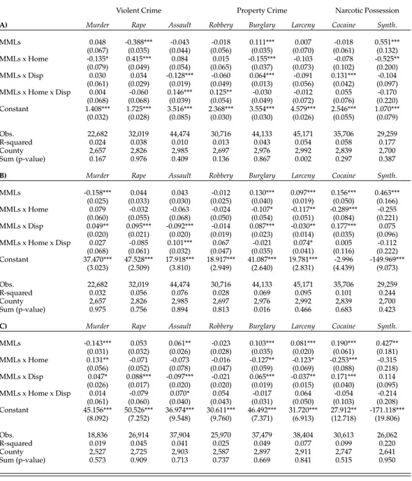
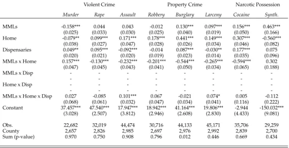
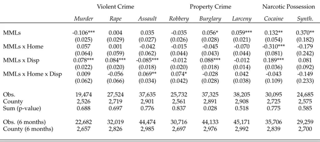
We find that a simple dichotomous indicator of Medical Marijuana Law (i.e. the average treatment effect on all the U.S. States that passed the policy) may mask crucial dynamics underlying the relationship between policy and crime. Assuming a homogeneous impact of policy on crime, regardless the action implemented, the dichotomous indicator of MML captures only the net effect of the regulatory tools put in place by the legislator. On the contrary, the policy decomposition in key dimensions allows to discover different results which suggests a heterogeneous effects on crime according to the specific regulatory actions put in place by the legislator.

In detail, for burglaries, larcenies, and cocaine drug possession, the mere application of demand side approach increases the crime in counties that passed the policy compared to counties without MML. While, the joint application of demand and supply approach — which establish legal sources for supply marijuana — may be able to realize a crowding-out effect on these offences. The findings support the idea that the licit competition on the marijuana market, triggered by the policy, could push out the illegal trade decreasing the crime. Finally, we find a net reduction in murders and a net increase in synthetic drug possession for the U.S. counties subject to the Medical Marijuana Law relatively to counties never passed the policy.

The second and the third essays assess the impact of law 92/2012, implemented in Italy in 2012 (the so-called Fornero reform), on different labour market outcomes. The law 92/2012 in-troduced numerous changes regarding employment relationships amending past discipline. First. It substantially changed the discipline concerning the dismissals in firms above 15 employees. The reform established that in case of unfair dismissal, the dismissed worker has no longer the right to be reinstated as in the pre-reform period and receives a monetary compensation that ranges between 12 and 24 months pay. Thus the reform significantly reduces the firing cost borne by large firms.

Second. Starting from January 2013, the Fornero reform also changed the discipline on ap-prenticeships concerning to the minimum duration of contract (no less than six months), the maximum number of apprentices that an employer can hire per each skilled worker (passed from 1:1 to 3:2), and the minimum number of apprentices that an employer must stabilize into permanent contracts for hiring a new apprentice (at least the 30% of apprentices hired in the last 12 months).

Third. The Fornero reform implemented a new incentive program in favour of employers that recruit (on fixed-term or open-ended contracts) or stabilize into permanent agreements a worker aged 50 or more years.

(13)

The second essay (carried out with Giovanni Pica) estimates the effect of employment protection legislation on the flow of monthly hirings on open ended contracts using the aforesaid labour market reform passed in Italy in 2012.

Much empirical research has focused on the effects of dismissal costs on labour market outcomes. The evidence suggests that EPL decreases employment inflows and outflows with little effect on employment and unemployment stocks. The reason is that firing costs act, in expected discounted value, as hiring cost reducing the willingness of the firms to both fire and hire workers (Bentolila and Bertola,1990;Blanchard and Portugal,2001).

The most recent studies identify the causal impact of employment protection on labour mar-ket outcome exploiting within-county variation in EPL either across firms (e.g. of different size) or workers (e.g. of different age and/or tenure). The essay presented is in the line with within-county approach which allows to better control for time-varying unobserved characteristics that may affect labour market outcomes (act as confounding factors) compared to cross-country analyses.

The presence of both treated and control firms observed before and after the policy — where the assignment of treatment depends in deterministic way from the number of workers employed — allows to implement a difference-in-difference approach jointly to a regression discontinuity design. We thus exploit the differential law change between firms with more and less than 15 workers comparing hirings in firms just above and below the 15 employee threshold before and after the reform (July 2012).

The analysis is based on monthly data drawn from Italian Social Security (INPS) record for the period 2012 and 2014. The data provide information on the number of newly hired workers by firms size, province, sector, contract type, age and gender at a monthly frequency. The findings suggest that the reform raises monthly hirings on open-ended contracts by about 5.1 percentage points. The quantification of results reveals that the reduction of dismissal costs after the reform have induced about 4000 hirings per month in firms with more than 15 workers relative to firms with less than 15 workers. The effect of the reduction in EPL is not homogeneous across workers’ types. The increase seems to be more pronounced for full-time, young, and blue-collar workers. Conversely, we find no significant effect on the number of conversions of temporary contracts into permanent ones.

The third essay evaluates the impact of labour policies aimed to improve the job possi-bilities for workers categorized as vulnerable (particularly in labour markets with stringent employment protection)7.

Given the increasingly complicated transition from school to works, the youth appear a group more vulnerable compared to the past. Here the apprenticeship contract performs a crucial role by improving the job possibility and the stability of young workers (Berton et al.,

2007;Casale et al.,2014).

7_{Evidences suggest that labour market prospects for youth and other marginal groups seem to worsen as a} consequence of stringent EPL (Allard and Lindert,2007;Bertola et al.,2007;Skedinger,2010).

(14)

Overview

At the same time, the low employment rates for older workers pushed most OECD countries to experiment specific employment protections with the purpose to protect them from unem-ployment or/and to improve their job finding rates (Chéron et al.,2011).

The Fornero reform intervenes by changing the discipline of apprenticeship in Italy and imple-menting a new incentive program for workers aged 50 or more years.

The reform asymmetrically acted on the apprenticeships by changing the discipline in firms with more than 10 employees leaving the rules for firms below 10 unchanged.

Likewise, the new incentive program for workers aged 50 or more years, passed with the Fornero reform, cut the hiring costs in firms that recruit workers over-50, leaving unaffected the costs for hiring workers under-50.

These discontinuities in the regulation as well as the simultaneous presence of treated and control groups observed before and after the policy allow to implement a difference-in-deference method jointly to a regression discontinuity design. This quasi-experimental method permits to evaluate the causal effect of reform on the monthly hirings of apprentices and workers over-50.

We thus exploit the differential law change in apprenticeships between firms with more and less than 10 employees, comparing the hirings and the conversions into open-ended contracts of apprentices in firms just below and above the 10 employees threshold before and after the reform (January 2013). Similarly, we compare the recruitments and the conversions into permanent contracts of workers with more and less 50 years before and after the reform. Also this analysis uses monthly data draw from Italian Social Security (INPS) record for the period 2012 and 2014.

The findings suggest that the change in apprenticeships increase the stabilization of appren-tices into open-ended contracts by about 3.9 percentage points in firms with more than 10 employees relative to firms with less than 10. We also find a positive association between law 92/2012 and the new recruitments of apprentices by about 7.1 percentage points in firms with more than 10 employees relative to firms with less than 10 employees.

The employer incentives for hiring and stabilizing the workers aged 50 or more years posi-tively affect the recruitments into open-ended contracts of workers over-50 relative to workers under-50 by about 1.6 percentage point. We also find a positive association between the incentive program and the hirings into fixed-term contracts of workers over-50 relative to workers under-50. Conversely, we don’t find effects for the conversions into open-ended contracts of workers aged 50 or more years.

The rest of thesis is organised as follow. Chapter1evaluates the impact of decriminal-ization of cannabis on crime exploiting the Medical Marijuana Laws ongoing in the U.S. States. Chapter2explores the relationship between employment protection legislation and the flow of monthly hirings on open-ended contracts using the law 92/2012 in Italy. Chapter3

assesses the impact of policies designed to improve the job possibility of workers categorised as vulnerable (i.e. youth and older) using the 2012 Italian labour market reform.

(15)

in the discipline, the identification strategy, the results, the sensitivity analysis and the conclusions.

(16)

(17)

Chapter 1

The Heterogeneous Effect of

Medical Marijuana Law

1.1 Introduction

In December 2012, 16 U.S. States and the District of Columbia passed a Medical Marijuana Laws (MMLs) interesting more than 90 millions of American citizen. Others 7 U.S. States approved MMLs between 2013 and December 2014.

Although possession and use of marijuana is still illegal under federal law, states are autho-rizing individuals to possess and use cannabis for medical or recreational use, loosening the punishments associated with this kind of felonies1. Moreover, states like Alaska, Colorado, Oregon, and Washington legalized possession and recreational use of marijuana by all indi-viduals over 21 years of age and several other states are considering similar mandates2. Medical use of cannabis became an increasingly contentious issue, in which the forces on either side of the prohibition-legalization debate see the introduction of Medical Marijuana legislations at states level as an initial step on the road to decriminalization of the drug. Federal government vehemently opposes state-level introduction of medical cannabis laws on a number of grounds, including a fear that they have the potential to increase use among the general population (especially young people) through sending the message that cannabis use is acceptable (Gorman and Huber,2007).

Wide acceptance and risk of consumption abuse triggered by Medical Marijuana legislations

1_{Federal agencies such}_{Drug Enforcement Administration}₍₂₀₁₅_{) continue to list marijuana as a Schedule I drug,} according to Controlled Substance Act (1970), like heroine. Substance are classified in Schedule I drugs because they have no known or accepted medical purpose and pose a risk for abuse.

Drug Enforcement Administration(2015) classify substance and certain chemicals used into 5 distinct categories or schedules depending upon the drugs acceptable medical use, abuses, or dependency potential. As schedule increase, the drug abuse potential decreases (i.e. Schedule V has the least abuse potential).

2_{Alaska legalized marijuana for recreational use in Measure 2 on November 4, 2015. Colorado legalized the sale} and possession of marijuana for non-medical uses on November 6, 2012, including private cultivation. Oregon legalized recreational use of marijuana for people ages 21 and older trough the Measure 91 on November 4, 2014. Washington permits anyone over 21 to carry one once of once, with Washington Initiative 502 in 2012.

(18)

1.1. Introduction

are spurring debates over the cost and benefits of these legalizations which might pour out their effects on broad social variables like public health, economics, and criminality.

A lot of opponents of marijuana laws for medical and recreational use, for instance, argue that they may induce increases in crimes.

This essay sheds light on the impact on crimes of Medical Marijuana Laws at the U.S. county level exploiting the heterogeneous regulatory actions adopted by policy makers. There have been four main approaches for the liberalization of the cannabis for medical purpose: the mere decriminalization of marijuana, the establishment of a mandatory patient registry, the permit to cultivate cannabis at home, the release of licence for selling cannabis in authorized dispensaries. The essay explores how each above dimension might influence the crime at county level.

These dimensions of MMLs can be classified in term of homogeneous choices of market design. We talk about demand side policies whether the regulatory action aims to the mere decriminalization of cannabis and supply side policies whether the regulation aims to provide legal sources of supply for marijuana.

This disaggregation of reform permits also to understand the potential transmission channel between Medical Marijuana Laws and crime. A demand side approach might induce an increase in the demand of marijuana without providing a legal source of supply. Hence, they induce individuals to address their increased demand towards illegal market (i.e. pusher or orga-nized crime), inflating profits and power of illegal activities. The boost of illegal trade may raise violence on drug markets through the so-called systemic transmission channel as defined inGoldstein(1985). In this sense, the demand side approach positively impact on crime. On the contrary, supply side approach could lead to a drop in crimes because they provide legal sources of supply marijuana through the cultivation at home and the selling in authorised dispensaries. This would trigger a licit competition on marijuana market which could push out the illegal trade. The result may be a reduction of crime.

According to this hypothesis, we expect that the demand side policies should be associated with an increase of crime, while the supply side policies should be able to reduce the crime. The net effect on crime of the two policies is an empirical matter.

To assess this we use a difference-in-difference approach considering the U.S. county level data on several types of crime among period 1994-2014.

This essay contributes to expand the previous literature regarding the impact on crime of the Medical Marijuana Laws in the United States for several reasons.

First. While the most of previous studies use crime data at State level, here we employ data at U.S. county level. This allows to catch the cross-county heterogeneity so far neglected. Second. We observe the crime for a longer time period (1994-2012) and for a wide sample of counties (96.5% of total) than the previous works, which usually analyse a shorter interval or a restricted group of States. The interval from 1994 to 2012 allows to investigate the crime trends both before and after the policies in each U.S. county.

Third. Most of previous studies analyse only two groups of felonies, violent and property crimes, according to classification ofUCR(2013). Here we evaluate effects of MMLs on

(19)

violent and property crime as well as on the felonies for narcotic possession. The offences referring to narcotic substances (different from the marijuana) helps to understand whether the gateway-effect happens upon the approval of Medical Marijuana Laws3.

Finally and crucially, our approach allows for a heterogeneous impact of policies on crime. Looking at approval timing of the Medical Marijuana legislations, we propose an origi-nal empirical model aimed to evaluate how each key dimension of MMLs may affect the crime. Classifying the regulatory actions like demand side policies (if they merely decriminalize cannabis) or supply side policies (if they provide legal sources of supply for marijuana), the model permits to test also the transmission channel between marijuana’s decriminalization and crime. Only few works consider the decomposition of policy (see, for instance,Pacula et al. 2015) but none of them implements a model or an interpretation similar to ours.

The remainder of the essay proceeds as follows. In Section1.2we summarize the limited research on Medical Marijuana Laws in United States. Section1.3provides background on Medical Marijuana Legislation analysing the key dimensions of reforms. In this section, we also explain our decomposition of policy and the transmission channel between MMLs and crime hypothesised. Details on empirical strategy are reported in Section1.5. The essay goes ahead to provide a description of our data (Section1.4) while Section1.6contains the results. Section1.7presents sensitivity analyses designed to test the robustness of results. We conclude with a summary of our finding and its implication in Section1.8.

1.2 Literature review

Economic and social literature has discussed the potential impact of drugs liberalizations in their different regulatory forms. Medical Marijuana legislations in United States are not kept out from these debates.

Medical researches provide clinical evidence on beneficial effect of marijuana for neu-ropathologies, to alleviate some symptoms associated with multiple sclerosis, and to help nausea associated with HIV (Corey-Bloom et al.,2012;Riggs et al.,2012;Wilsey et al.,2013). Others support the view that the marijuana legalizations could be associated with economics improvements. On the one hand, reforms may save taxpayers’ money reducing costs associ-ated with the arrests and detentions of non-violent individuals involved in the marijuana trade. On the other hand, they may permit to tax the trade of cannabis and its derivatives4. Resources which could be allocated towards public schools, infrastructure, and young cam-paigns on conscious use of narcotic substances.

3_{With the term gateway-effect (also called gateway theory and gateway hypothesis) refers to the phenomenon according} which the use of less deleterious drugs precedes, and can lead to, future use of more dangerous hard drugs or crime. It is often attributed to the earlier use of one of several licit substances, including tobacco or alcohol, as well as cannabis (seeDeSimone 1998).

4_{During the first month of entry in force of law, the sales of recreational marijuana in Colorado produced around} 3.5 million dollars in taxes (Alford,2014).

(20)

1.2. Literature review

Opponents of marijuana decriminalization argue that widely use of cannabis may lead to worse schooling and work outcomes.DeSimone(1998,2002), for instance, finds that use of each drugs (still marijuana) reduces the likelihood of employment, while increases the proba-bility to use of cocaine evidencing the presence of gateway hypothesis.Yamada et al.(1996) reveals a significant adverse effects of cannabis use on high school graduate rates, while

McCaffrey et al.(2010) observed that cigarette and marijuana smoking could be associate with greater high school dropout rate.

Studies regarding the Medical Marijuana Laws can be distinguished in two branches: those which analyse the effects on consumption of marijuana and those which analyse the potential impact on crime. There are many works investigating the relationship between MMLs and consumption of marijuana, alcohol or others narcotic substances in United States while there are few researches on the relationship between MMLs and crimes5_.

Among them, onlyPacula et al.(2015) employ a decomposition of MMLs in key dimensions in order to inspect the effect of policy on recreational use of marijuana. Their findings suggest a heterogeneous impact of laws depending to the specific regulatory actions put in place by the legislator6_{. This suggests that to fully understand the effect of Medical Marijuana Laws}

we must take into account the potential heterogeneity associated with the single regulatory actions. This might be true for the impact on marijuana’s consumption as much as that on crime.

About the relationship between MMLs and crime,Morris et al.(2014) find no significant impact with the exceptions of homicides and aggravated assaults for which they reveal negative relationship.Gavrilova et al.(2015), limiting analysis for the U.S. states on border with Mexico, find a significant negative impact of MMLs on violent crime with strong effects on robberies and homicides. Moreover, they identify a not clear effect of dispensaries and home cultivation on crime. However, using also Supplementary Homicide Reports (SHR) data, they confirm the fall of homicides (originated from decreasing in murderers among juvenile-gang). Alford(2014) finds that selling marijuana in dispensaries may have positive effect on property crimes while she doesn’t find statistically significant effect for home cultivation. Finally,Anderson et al.(2011) find that legalization in U.S. states decrease traffic fatalities, particularly those involving alcohol. They observe also sharp decreasing in alcohol consump-tion suggesting that alcohol and marijuana are substitute.

5_{Referring to the impact on cannabis consumption,}_{Khatapoush and Hallfors}₍₂₀₀₄_),_{Gorman and Huber}₍₂₀₀₇_), andHarper et al.(2012) find not significant impact of MMLs on marijuana use. Instead,Anderson et al.(2011), analysing passage of laws in Rhode Island, Vermont, and Montana, finds a positive and significant relationship between policy and marijuana use among individuals aged 18 or older. Conversely, the effect seems to be negligible among the minors (aged 12 to 17). Using marijuana arrest and marijuana treatment admission like proxies for use of cannabis,Chu(2012) evidences a strong positive effect of MMLs on both outcomes, suggesting a positive association between MMLs and illegal use. Other examples areChu(2012) andPacula et al.(2015).

6_{The key dimensions considered in}_{Pacula et al.}₍₂₀₁₅_{) are similar to ours: actions which merely decriminalize} cannabis, the establishment of a mandatory patient registry, the permit to cultivate cannabis at home, and the licence for selling cannabis in authorized dispensaries. They find that the simple medical allowances and patient registration requirement have a negative impact on recreational marijuana use, whereas legally protected dispensaries positively influence recreational use.

(21)

Although the aforesaid authors analyse the relationship between MMLs and crime for the different key dimensions of policy (as inPacula et al. 2015), they neglect both the cross-effect on crime ascribable to the combined approval of two or more dimensions and the timing in which the specific dimension is put in place by the legislator. This, jointly with the use a county level data, represents the main distinctive element of our work compared to previous literature. The essay recognizes that not all medical marijuana policies are homogeneous but policy dimensions are important and not static. We exploit the variation in the tim-ing of the core elements of MML policy (shown in Table1.1) to assess whether particular forms of regulation are more relevant to estimate the impact of MMLs on crime in each county.

Other studies look at the link between the marijuana market and the trade of other illicit drug in order to assess the so-called gateway drug hypothesis, according which marijuana is complementary to demand of others drugs. Empirical evidences don’t clarify if this phe-nomenon is present in the context of Medical Marijuana legislations.Chu(2013) finds no significant effect on the arrests for possession of other drugs. However, using Treatment Episode Data Set (TEDS), he finds that MMLs may decrease heroine treatment admissions. This would contradict the complementary between the marijuana and other drugs. On the contrary,Choi(2014), examining the impact of MMLs on various risky health behaviours, finds positive association between selling marijuana in dispensaries and use of other narcotic substances (no-marijuana) suggesting the presence of gateway hypothesis. She also finds negative link between allowing home cultivation and driving under the influence of drugs.

1.3 Evolution of MML in the U.S.

Since 1996 numerous U.S. States issued policies recognizing the medicinal value of mari-juana and providing a legal defence for patient who used marimari-juana under recommendation of a physician. The set of juridical rules on therapeutic consumption, production, and distri-bution of cannabis are noted as Medical Marijuana Laws (MMLs). The purposes of MML was pain reduction for patients where the States allow doctors to prescribe marijuana as a pain killer7. However, the list of illness is often broad and it is so difficult to verify whether pain complaints are real. This generated wide possibilities for recreational use of marijuana masked like therapeutic consumptions (Chu,2012).

In December 2012, 16 U.S. States and District of Columbia decided to ratify Medical

Mari-7_{Each state instituted a list of illness allowed to use marijuana for authorized patient. Among these, there are} anorexia, arthritis, cachexia, neurodegenerative diseases, cancer, HIV/AIDS, chronic pain, glaucoma, migraines, persistent muscle spasms, severe nausea, seizures, and sclerosis. However, in many states is consented to use cannabis also for conditions related with stress or depression state. Patients can legally possess marijuana up to a fixed amount, which differs by U.S. states (Chu,2012;Pros & Cons,2015). In most cases, the law allows a written or oral recommendation by a physician to use as defence in the case the patient should be arrested on charge of cannabis possession.

(22)

1.3. Evolution of MML in the U.S.

juana Law involving more than 90 millions of Americans (around 30% of U.S. population). Between January 2013 and December 2014, others 7 states moved towards the same direction8. U.S. map permits to realize how MMLs are developing among American States (Figure1.1). Details of legislation ratified in each U.S. State are reported in Table1.19.

Figure 1.1:Medical Marijuana Law in U.S. States (1994-2012).

Note:The map omits the States of Alaska and Hawaii which passed the Medical Marijuana Law between 1994-2012. In dark blue are drawn U.S. state adopting MMLs, while in light blue ones never adopting reforms.

Voter referendum have represented the main tool to approve MMLs for many States between 1996 and 2000. However, referendum provides little specific guidance about decriminaliza-tion and acceptable source of supply for marijuana (i.e. possibility of cultivadecriminaliza-tion, selling authorization, and so on). This has often flowed into legislative, administrative and judicial actions (in many cases competing one another) aimed to better specify the original reform (Pacula et al.,2015). In detail, they have established i) a patient registry systems for individu-als who assume marijuana, ii) the possibility to cultivate cannabis at home, and iii) to sell marijuana in the authorized dispensaries. Since each State can choose the specific actions to adopt, we now observe a heterogeneous framework among the American States in term of measures in favour of marijuana (see Table1.1).

Most of previous literature ignores this heterogeneity by evaluating the policy through a simple dichotomous distinction between States adopted MML and those that never passed the marijuana decriminalization. This could explain in part the inconsistency of past liter-ature about the causal effect between Medical Marijuana legislations and crime. Indeed, the simple dichotomous indicator may mask important heterogeneous effects linked to the

8_{Connecticut (2013), Illinois (2014), Maryland (2014), Massachusetts (2013), Minnesota (2014), New Hampshire} (2014) e New York (2014).

9_Table_1.14_{in Appendix contains the list of States interested by the Medical Marijuana Law with the legislative} procedures implemented, and application methods used by policy maker.

(23)

specific actions put in place by the legislator in each State (Pacula et al.,2015).

The approach chosen in this essay neglects the dichotomous identification of MMLs, looking closelyPacula et al.(2015) for the decomposition of Mediacal Marijuana Laws. However, there are several elements of distinction in our approach. First, we are interested to the impact on crime of MMLs, whilePacula et al.(2015) inspect the relationship with marijuana consumption. Second, we remodulate the decomposition adopted byPacula et al.(2015) classifying regulatory actions of policy makers into homogeneous choices of market design. Since it is reasonable to think that different regulatory actions produce different effect on markets, we need to assess them distinctly.

A. POLICYDECOMPOSITION ANDTRANSMISSIONCHANNEL.

Pacula et al.(2015) distinguishes three specific dimensions of State MMLs that could influence the general availability and social norms surrounding marijuana use: i) require patient registry systems10; ii) allow home cultivation11, and iii) legally permit dispensaries12. In this essay, we consider a further dimension of MMLs thanPacula et al.(2015): dates in which each state permits consumption of marijuana for medical practices.

Note that, it can differ from patient registry system dimension because many states imple-ment a mandatory register after the first decriminalization. Some States either do not have a patient registry system (e.g. Washington) or have a voluntary system of registration (e.g. California).

Cutting the Medical Marijuana Law in single regulatory actions can be useful to understand how choices to design the legal marijuana market may affect social variables like crime, health, and so on.

Medical allowed (or mere decriminalization) and mandatory patient registry system may be classified like dimensions addressed at control the consumption of marijuana but without to provide ways in which new consumers can obtain the substance: on legal or on illegal market? Hence, we see them like a demand side policy regulating the marijuana market. On the contrary, dimensions referring to possibility of cultivation and selling marijuana in dispensaries may be classified like actions addressed to provide a legal sources of supply. So, they could be seen like a supply side policy.

10_{Patients or caregivers, affected by illnesses for which granted the use of cannabis, are obliged to register in a} patient registry established by the authorities, which issue a special certificate (renewable annually). Possession of certificate is a requirement to not prosecution of crimes, like possession and consumption of marijuana.

11_{Not only patients can cultivate marijuana for personal use but laws allow caregivers (most of whom are patient} as well) to grow and provide marijuana to patients on a non profit basis.

12_{Dispensaries are stores specializing in the sale of marijuana and its derivatives for authorized individuals} (patients). They are typically organized as co-operative association (collectives). Members of the collective can either be producers, consumers or both. In same state producers can be a member of multiple dispensaries allowing them to scale up their production substantially, but in other states this is not allowed (Gavrilova et al.,2015).

Table1.15in Appendix shows when and in which U.S. States each dimension of Medical Marijuana Laws was been implemented.

(24)

Through the demand side policy (i.e. the mere decriminalization or mandatory patient registry) the policy maker increases the demand of marijuana by encouraging the entrance on marijuana market of consumers so far discouraged to use cannabis just because it was a crime13. Moreover, these policies may reduce both health and legal individual costs associ-ated to consumption of marijuana, further pushing up the demand of cannabis14.

Through the supply side policies the policy maker instead provides tools to produce and allocate cannabis on market through legal channels (thanks to possibility of home cultivation and selling in dispensaries). Also these policies may increase the consumption of marijuana since they may reduce individual research costs, rise social approbation of cannabis, and decrease the marijuana price15_.

Our codification of reforms permits to explain also the transmission channel between the Medical Marijuana Law and crime. FollowingGoldstein(1985), there are three main mech-anisms through which narcotic drugs can affect criminal activities. Psycho-pharmacological channel, according to which drugs may increase aggression of users and thus induce vio-lence16. Economic channel, according to which users may resort to crime in order to finance their drug habit17. Systemic channel, according to which disputes between drug market participants are solved with violence because drug agreements cannot be enforced in the courts18.

Naturally, Medical Marijuana Laws may affect crime through each aforesaid transmission channel. Taking into account the specific regulatory actions approved in in each U.S. State, we can give empirical evidence also on the transmission channel.

13_{Standard economics theory of narcotic substance use postulate that consumers get utility from consuming} intoxicating substance, just like other goods. Their consumption is constrained by the income available to the individual, and price of the substance (as any others goods) but also by legal and health risks associated with using the illegal intoxicating substance (Grossman,2005;Pacula et al.,2010). The illegal nature of the drug generate also a search costs associated with trying to find and access the substance (Galenianos et al.,2012). These peculiarity costs should reduce the marginal utility of consuming marijuana and hence lower overall use of cannabis for a given price. Therefore, the decriminalization of cannabis associated with MMLs may stimulate the demand of marijuana. 14_{Legal costs because demand side policy permits to legally use marijuana. Health costs because this policy could} bring individuals to associate lower harm to consumption of marijuana, since it is a medicine.

15_{Numerous studies reveal positive relationship between medical legalization and marijuana consumption in} United States (Anderson et al.,2015;Cerdá et al.,2012;Choi,2014;Pacula et al.,2010).Walsh et al.(2013) show the same pattern in Canada. See alsoPacula and Sevigny(2014) andPacula et al.(2015).

16_{The most relevant substances in this regard are probably alcohol, stimulants, barbiturates, and phencyclidine} (PCP). Reports which sought to employ a psycho-pharmacological channel to attribute violent behaviour to the use opiates and marijuana have been largely discredited. Indeed, several opioid substances may have a reverse effect on users and ameliorate violent tendencies, controlling their violent impulses (Goldstein,1985).

17_{Robberies represent typical way to support costly drug use. Heroine and cocaine are the most relevant substances} in this category because they are expensive drug typified by compulsive patterns of use (Goldstein,1985).

18_{This channel refers to traditionally aggressive patterns of interaction within the system of drug distribution} and use. Examples can be: disputes over territory between rival drug dealers; assaults and homicides committed within dealing hierarchies as a means of enforcing normative code; robbery of drug dealers and the usually violent retaliation by the dealer; punishment for failing to pay one’s debts, and so on. Since criminal entrepreneurs operate outside the law regardless by kind of drug traded, this channel may apply at all narcotic substances, such as marijuana, cocaine, heroine, etc. (Goldstein,1985).

(25)

B. TIMING OF REFORMS ANDPOLICYINDICATORS.

U.S. States regulated the legal market of marijuana in heterogeneous way between 1994 and 2012 (see Table1.1). Since the effective date of the legislations often occurs later than the enactment date, we followPacula et al.(2015) which employ the effective dates of State laws to operationalize the policy indicators used in empirical analyses.

Table1.1allows to rebuild the timing approval of Medical Marijuana State Laws for each aforesaid key dimension of policy.

First dimension is the so-called Medical Allowed (Column 3). It identify the States which passed the decriminalization of cannabis or/and established a mandatory patient registry systems between 1994 and 2012. Although they ideally represent distinct regulatory acts, decriminalization and patient registry systems actually are jointly implemented (see Table

1.15in Appendix). Therefore, we choose to employ an unique policy indicator for both of them. Columns 4 refers to the dimension Home Cultivation. It identifies the States which provide legal protection for patients or caregivers to cultivate cannabis at home for medical purpose19. Column 5, called Legal Dispensaries Operating, identifies States that can be legally interpreted as providing protection for dispensaries to operate within the State. We follow

Pacula et al.(2015) for identifying the actual operating dates. Table1.1shows both approval and operating dates of laws for dispensaries20.

Looking at approval timing of MML dimensions in Table1.1, we find that demand side policies (i.e. decriminalization or patient registry system) are systematically carried out before than supply side policies (i.e. home cultivation or dispensaries). This suggests that the dichoto-mous indicator of MMLs (which reflects the dates of first State regulatory action in favour of decriminalization of cannabis for therapeutic uses) coincides, de facto, with our demand side policy indicator. Hence, it ignores the potential heterogeneous impact of policy on crime induced by subsequent and different regulatory State acts aimed to provide legal sources of supply marijuana (i.e. supply side policies).

Table1.1represents the guideline to build policy indicators (treatment variables) applied in our econometrics analysis. These variables have the purpose to distinguish States adopting single dimensions of Medical Marijuana Laws from states never adopting any form of cannabis decriminalization for therapeutic uses.

Although the Medical Marijuana Law passed at State level, theUCR(2013) dataset allows to explore the impact of MMLs on crime at the county level. Consequently, also our policy

19_{Note that the laws vary across the States also referring to the number of cannabis plants that can be grown at} home by patients or their designated caregiver. Table1.14in Appendix provides details.

20_{The clarification between approval and operating date of the dispensaries is not trivial. There are States, such} as Washington and Michigan, where there are operating dispensaries in certain municipalities even though the State does not legal permit them. On the contrary, there are States which issued legal licence for dispensaries but actually they don’t have operating dispensaries or they operate for a couple of years thereafter (Pacula et al.,2015). Therefore, we identify the State like allowed dispensaries if it there are operating dispensaries (whether legal or illegal way) within the State. It’s reasonable to think that the dispensaries exert no effect on crime if they are not actual present within the States.

(26)

Table 1.1:Timing of Medical Marijuana State Laws (1994-2012)

U.S. First Medical Home Legal Dispensaries

State Reform Allowed Cultivation operating

Alaska 1999 1999 1999 - -Arizona 2010 2010 2010 2012 (2010) California 1996 1996 2010 2003 (2003) Colorado 2001 2001 2001 2005 (2000) Delaware 2011 2011 - - (2011) District of Columbia 2010 2010 - - (2010) Hawaii 2000 2000 2000 - -Maine 1999 1999 1999 2011 (2009) Michigan 2008 2008 2008 2009 -Montana 2004 2004 2004 2009 (2009) Nevada 2001 2001 2001 2009 -New Jersey 2010 2010 - 2012 (2009) New Mexico 2007 2007 2007 2009 (2007) Oregon 1998 1998 1998 2009 -Rhode Island 2006 2006 2006 - (2009) Vermount 2004 2004 2004 - (2011) Washington 1998 1998 1998 2011

-Source:Pros & Cons(2015);Pacula et al.(2015);Alford(2014).

Note: The table presents MMLs and their key dimensions up to year 2012. Second column show the date when the law became active. Third column shows date of decriminalization for medical use. Fourth column shows whether there is a statewide allowance for home cultivation, with date if present, otherwise (-). Fifth column give the same information about the dispensaries. In parenthesis, there are date in which legally dispensaries are allowed. There

are cases where the dispensaries are operating although there are not any act concern them, symbol ( - ).

indicators will refer to the U.S. Counties.

Assuming that the specific dimension j of policy carries out at time t=k and each county is observed before and after the change. Let sibe the variable identifying if county i belongs

to group of counties subject to dimension j of MML. So si assumes value 1 if county is

subjected to the dimensions j of MMLs between 1994 and 2012, otherwise it assumes zero value. Formally, the policy indicator (or treatment variable) is defined as:

d_i,tj =    1, i f si=1 and t>k 0, otherwise

where i identifies the county, t indexes the time, and j identifies the specific dimension of MMLs.

We consider three policy indicators corresponding to columns 3, 4, and 5 of Table1.1. Variable dMML, assuming value 1 if county i at time t has any form of demand side policies. Variable dHOME, assuming value 1 if county i at time t allows home cultivation by approved patient. Variable dDISP, assuming value 1 if county i at time t has operating dispensaries within belonging state.

(27)

Table1.2reports descriptive statistics of aforesaid treatment variables. Coverage of sampled counties is almost complete: on 3,144 U.S. county we have data for 3,034 (96.5%). Around of 16.3% of counties are subject to whichever form of decriminalization of cannabis for thera-peutic use (as results from the mean in the Table1.2).

All the counties adopt MMLs through a demand side policy. In fact, the dichotomous indicator of policy (or the first reform) is equal to indicator of demand side. Well we can refers to them indistinctly. Roughly the 15% of counties provides a legal supply source of marijuana to authorized patients (i.e. supply side policies), through the home cultivation (15.5%) or the sale in dispensaries (14.6%).

Table 1.2:Treatment Variables (descriptive analysis)

VARIABLES N Mean Var.

Dichotomous Indicator of MMLs∗ 3,034 0.163 0.137 Demand Side Policies 3,034 0.163 0.137 Home Cultivation (Supply Side) 3,034 0.155 0.131 Dispensaries Licence (Supply Side) 3,034 0.146 0.125

Note:∗The dichotomous indicator of MMLs is built referring to the dates of the first regulatory act in favour of marijuana for therapeutic purpose. Statistics are reported for each dimension of Medical Marijuana legislation used in econometrics analysis. Demand side policies indicator refers to the counties which adopted or a mere decriminalization of cannabis or established a mandatory patient registry system. Supply side policy indicator is split in home cultivation and dispensaries dimensions. Since each county policy indicator is a dummy variable, their mean represents the percentage of counties which adopt that specific regulatory action.

1.4 Data

The analysis uses the Uniform Crime Reporting Program Data (UCR,2013). The dataset contains the number of arrest by type of offence (like murder, rape, robbery, aggravated assault, burglary, larceny, auto theft, and arson) at the county level. TheUCR(2013) also reports arrest for additional crimes such as forgery, fraud, vice offences, and drug possession or sale.

The data were originally collected by Federal Bureau Investigation (FBI) from reports sub-mitted by agencies and states participating in the UCR Program. We exploit data from UCR Program provided by Inter-university Consortium for Political and Social Research (ICPSR,

1994-2012) for the years 1994 through 2012.

The use of arrest data as proxies of crimes is the norm in criminology researches.

Since a person may be arrested several times, each arrest count does not necessarily represent a single individual.

(28)

1.4. Data

serious offences21. Hence, minor crimes are reported only when they happen alone. We use arrests since 1994 because there was a change in the data collection methodology after the 1993 (see codebook of data) which caused a break in series. Therefore, data from earlier years should not be compared to data from 1994 and subsequent years. This doesn’t trouble present work because the first Medical Marijuana legislation happened in California in 1996. Since participation in the UCR Program is generally voluntary, many agencies might not report data in every months for every years for one or more categories of crime. In order to distinguish true zero from missing values, FBI provides a coverage indicator in conjunction with the arrest variables. We follow the procedure illustrated in codebooks published with the data to correct for this issue.

As common in the criminology literature (seeCarpenter 2007), we use observations only if the agencies report arrests for at least six months in that year.

After adjustments, we have 473, 344 observations on arrests classified by type of crime. Data refers to 3, 034 U.S. counties, that’s the 96.5% of total counties, among the periods 1994-2012.

According to FBI classification, we can pool felonies in violent, property, and narcotic crimes (Handbook-UCR,2004). Present analysis is based on eight crime variables, three belonging to violent crimes (murder, rape, and aggravated assault), three belonging to property crimes (robbery, burglary, and larceny), and two belonging to narcotic crimes (cocaine and synthetic narcotics possession22). Details on each crime variable are reported in Appendix (seeCrime

Variables). Variables are chosen in order to estimate how Medical Marijuana legislation may

affect crimes at county level trying also to understand whether there was a heterogeneous impact among different kind of crimes (seeGoldstein,1985).

Finally, we consider several socio-economic variables (per-capita GDP, labour force and unemployment) for the purpose to use them like controls in our empiric strategy. They come from theU.S. Bureau of Economic Analysis(2014) andU.S. Bureau of Labor Statistics(2014).

A. DESCRIPTIVESTATISTICS.

In this subsection we briefly exhibit the trend of crime in United States trying to underline whether there was a different pattern between the counties subject to the Medical Marijuana legislation and counties that never approved policy. This is crucial in a difference-in-difference approach where the common trend assumption among treated and control groups is a key identification condition.

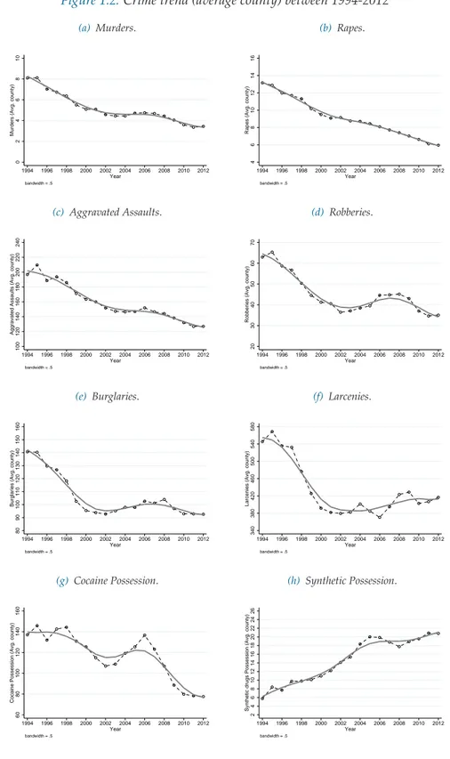
Crimes in United States had a significant fall among 1994-2012 as observable for murder, rape, aggravated assault, robbery, larceny, burglary, and cocaine possession. In sharply contrast, arrests for synthetic narcotics possession strongly increase. This is true both for total crimes

21_{For instance, in the case of arrest for murder and drug trafficking UCR reports only the murder, while the felony} concerning narcotic substances are not reported.

22_{In detail, cocaine variables includes the possession of opium, cocaine, and all their derivatives like morphine,} heroine, and codeine. While, synthetic narcotics consists of the possession of demerol, and methadone.

(29)

in United States and for average crime at county level (Figure1.2).

Table1.3shows descriptive statistics for all crime variables at U.S. county level. We report statistics with and without zero values because, following the past literature, our baseline formulation of empirical model (Equation1.4) considers crime (dependent) variable as logarithm. Thus, it refers only to non-zero observations.

Although this is not a problem for state level data, since there are not zeros, it cannot be neglected with county level data. Indeed, murder, rape, robberies, cocaine, and synthetic drug possession have significant percentages of zero observations. In Section1.7, we test the robustness of our results also to introduction of zeros.

Almost all the mean values of crime variables are sufficiently high for ordinary least square (OLS). We stress this because with counts data (like in criminology) may happen to have a small average count (e.g. less than 5), troubling for OLS regression analysis that assume nor-mal distribution in error around the expected average (Agresti,2007;Piquero and Weisburd,

2010). Since most of crime variables present high average count (e.g. greater than 20), OLS represents the best estimation too (see Table1.3).

However, felonies like murder, rape, and synthetic drugs possession have average count relatively low, making the OLS less efficient. In Section1.7, we test the robustness of our results also estimating a non linear model for count data.

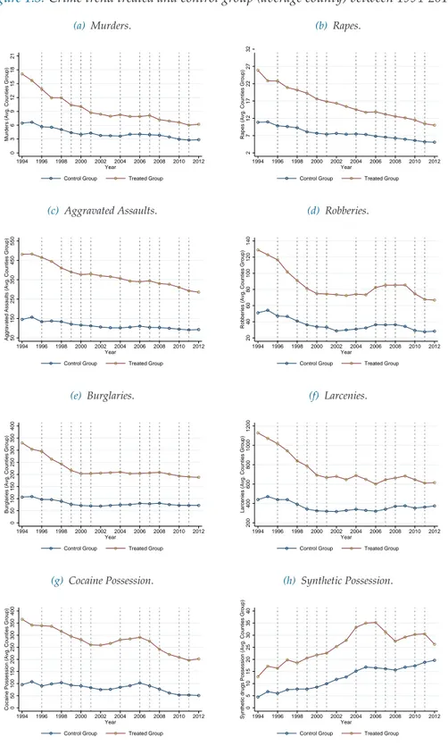
We want to verify whether the common trend assumption holds. For this purpose we compare, in Figure1.3, the evolution in crimes for treated and control counties. The vertical lines in Figure1.3represent dates in which U.S. states endorsed the first reform towards a marijuana liberalization for therapeutic use.

Since Medical Marijuana State Laws are not passed in the same year (see vertical lines) we have a multi-treatment during the period 1994-2012. This doesn’t consent to clearly appreciate, through the graph, the mean change in crime recorded in the treated counties relative to control counties over the period before and after the policy.

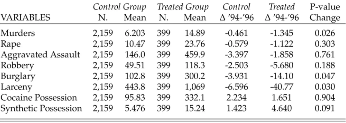
Crime trend among two groups doesn’t seem to radically differ specially in a common pre-treatment period (1994-1996). Nevertheless, counties which ratified the Medical Marijuana Law are characterised by higher criminality rates than the ones which never passed decrimi-nalization of marijuana. This evidence is true for all crimes analysed and it interests also the pre-treatment period 1994-1996 common to all counties, as showed in Table1.4.

This might suggest that reforms may have been the consequence of periods with high crimi-nality rate making policy endogenous. The test on mean change in crime among common pre-treatment period (i.e. 1994-1996) between treated and control counties reveals that there are not difference statistically significant at 99% of confidence level (last column, Table1.4).

(30)

1.4. Data

Figure 1.2:Crime trend (average county) between 1994-2012

(a) Murders. 0 2 4 6 8 10

Murders (Avg. county)

1994 1996 1998 2000 2002 2004 2006 2008 2010 2012 Year bandwidth = .5 (b) Rapes. 4 6 8 10 12 14 16

Rapes (Avg. county)

1994 1996 1998 2000 2002 2004 2006 2008 2010 2012 Year bandwidth = .5 (c) Aggravated Assaults. 100 120 140 160 180 200 220 240

Aggravated Assaults (Avg. county)

1994 1996 1998 2000 2002 2004 2006 2008 2010 2012 Year bandwidth = .5 (d) Robberies. 20 30 40 50 60 70

Robberies (Avg. county)

1994 1996 1998 2000 2002 2004 2006 2008 2010 2012 Year bandwidth = .5 (e) Burglaries. 80 90 100 110 120 130 140 150 160

Burglaries (Avg. county)

1994 1996 1998 2000 2002 2004 2006 2008 2010 2012 Year bandwidth = .5 (f) Larcenies. 340 380 420 460 500 540 580

Larcenies (Avg. county)

1994 1996 1998 2000 2002 2004 2006 2008 2010 2012 Year bandwidth = .5 (g) Cocaine Possession. 60 80 100 120 140 160

Cocaine Possession (Avg. county)

1994 1996 1998 2000 2002 2004 2006 2008 2010 2012 Year bandwidth = .5 (h) Synthetic Possession. 2 4 6 8 10 12 14 16 18 20 22 24 26

Synthetic drugs Possession (Avg. county)