CFD modelling of the Borexino solar neutrino detector : investigation of the inner vessel fluid-dynamics and polonium concentration

(1)

Politecnico di Milano

SCHOOL OF INDUSTRIAL AND INFORMATION ENGINEERING Master of Science – Energy Engineering

CFD Modelling of the Borexino Solar

Neutrino Detector:

Investigation of the Inner Vessel

Fluid-dynamics and Polonium Concentration

Supervisor

Prof. RICCARDO MEREU

Co-Supervisor

Ing. VALENTINO DI MARCELLO

Candidate

ROMOLO BENATI – 892769

(2)

(3)

Acknowledgements

I would like to thank, fist of all, professor Mereu, who taught me what does it mean to work in a professional environment. Second, thank you Valentino for the constant and clear support.

Thanks to my parents and my family, you pushed me in every moment towards the growth.

Thank you very much to all the colleagues who shared with me this travel through the Politecnico di Milano. Thank you Matilde and VW12. A hug to Davide, Fabi, Baba, Marti, Gico, Paolo, Nico and the other 200 people. Good luck.

Thank you Camilla and all the great people met in Norway. A special thanks to mon frère francais and mi hermana mexicana, Alexis and Alajandra.

Thank you Mattia for the help with LA_{TEX. . . and for the rest. Thank you Agnese for}

the English. Thank you Sbocc and the artists. Thanks to Villa Oliva, that hosted me for the writing.

Of course, thanks to the GNAM Society.

(4)

(5)

Sommario

Borexino è un rilevatore di neutrini ad alta precisione situato nei Laboratori Nazionali del Gran Sasso, in Abruzzo. Livelli straordinari di radiopurezza sono stati raggiunti ed hanno permesso la misurazione di neutrini prodotti da diverse reazioni di fusione nucleare nel Sole. In ogni caso, la presenza di contaminanti nel suo Inner Vessel (IV), come bismuto e polonio, genera eventi di fondo che impediscono il rilevamento dei neutrini originati nel ciclo CNO. Il moto di questi contaminanti è strettamente collegato alla fluidodinamica; è stato ricercato un metodo che permetta quindi di mettere in relazione le condizioni termiche esterne a Borexino ed i movimenti del fluido contenuto. Le asimmetrie della temperatura dell’aria che circonda il rilevatore sono la causa della convezione naturale interna. Un modello CFD bidimensionale ed uno tridimensionale sono stati ideati affiché possano riprodurre la fluidodinamica dell’IV. Le sonde di temperatura, posizionate sia esternamente sia internamente a Borexino, hanno fornito i dati di input per il software; la posizione esatta di un sensore rimane però sconosciuta e crea lieve incertezza nelle condizioni al contorno. I dati considerati sono relativi ad un periodo tra Gennaio e Febbraio 2017. Conseguentemente, il modello matematico e quello numerico sono descritti. Diverse analisi di sensitività, sulla configurazione della mesh e sul time-step, sono state portate a termine con lo scopo di incrementare la precisione dei risultati e di capirne la validità. Il modello 2D mostra la presenza di flussi orizzontali stratificati. Il 3D conferma il trend e rivela che il fluido sta effettivamnete ruotando attorno all’asse verticale. Le componenti verticali della velocità sono in entrambi i casi molto deboli e probabilmente legate al rumore numerico; nel sistema tridimensionale inoltre, dei movimenti ascensionali al bordo sono rilevati, in accordo con passate osservazioni sulla migrazione del polonio. Sempre nel caso 3D, la maggiore dimensione media della cella porta a velocità di un ordine di grandezza più elevato rispetto al 2D. Questo fatto ovviamente influenza la distribuzione finale di polonio. In quel periodo, la concentrazione reale di 210Po vede un minimo nella parte alta del volume preso in esame. Mentre il modello di trasposto bidimensionale ha ottenuto una buona corrispondenza con i dati misurati, sia qualitativa sia quantitativa, quello tridimensionale presenta una concentrazione di gran lunga superiore. E’ possibile però affermare che i risultati 3D stiano gradualmente avvicinandosi a quelli 2D, un ruolo fondamentale è giocato dalla griglia computazionale.

Parole chiave: Computational Fluid Dynamics Rilevatore di neutrini Convezione naturale Borexino

(6)

(7)

Abstract

Borexino is a high-precision neutrinos detector located in the Laboratori Nazionali del Gran Sasso, in Abruzzo. Extraordinary radio-purity levels have been reached and permitted to measure neutrinos fluxes produced by several fusion reactions occurring in the Sun. Anyway, the presence of contaminants in its Inner Vessel (IV), such as bismuth and polonium, generates background events which can worsen the detection of the neutrinos related to the CNO-cycle. The motion of these contaminants is strictly linked to the fluid-dynamics; a method to correlate the external thermal environment and the internal fluid movements is being searched. The temperature asymmetries of the air surrounding the detector are the drivers of the inner natural convection. A bi-dimensional and a tri-dimensional Computational Fluid Dynamics (CFD) models were designed in order to reproduce the fluid-dynamics of the IV. The temperature probes, arranged outside and inside Borexino, provided the input data for the software; different data interpolations were used because of the uncertain position of one particular probe. Data from a period among January and February 2017 have been considered. Thus, the mathematical and the numerical models are carefully described. Several sensitivity analysis, on the mesh configuration and on the time-step, have been then computed with the purpose of understanding the validity and increasing the precision of the results. The 2D model shows the presence of horizontal stratified flows. The 3D model confirms the trend and reveals that the fluid is spinning around the central vertical axis. The vertical velocity components in the bulk are in both cases very weak and probably related to numerical noise; in the tri-dimensional system anyway, some vertical movements at the border are present and are in agreement with previous observations of the polonium migration. In the 3D case also, the larger average cell size generates a velocity intensity of a higher order of magnitude compared to the 2D. This certainly affects the final polonium distribution. In that period, the 210Po real concentration shows a minimum in the topmost part of the volume. While the bi-dimensional transfer model obtains qualitatively and quantitatively a good match with the measured data, the tri-dimensional one presents an extremely higher concentration. It is possible to say that the 3D results are slowly approaching the 2D ones; key role is played by the computational grid.

Keywords: Computational Fluid Dynamics

Neutrino detector Natural convection Borexino

(8)

(9)

List of Figures

Figure 1.1 Schematic drawing of the Borexino detector . . . 4

Figure 1.2 PC and PPO molecules . . . 5

Figure 1.3 DMP molecule . . . 6

Figure 1.4 LTPS probes positions. Division by phase of installation. . . . 9

Figure 1.5 Sample of the TIS material . . . 10

Figure 2.1 Initial temperature distribution for the IV. Picture taken from the 3D convective simulation of the IV (see below) of February 2017. 12 Figure 2.2 Water Ring model structure. . . 14

Figure 4.1 Boundary layer comparison for the 2D cases. . . 20

Figure 4.2 Boundary layer meshes comparison. . . 21

Figure 4.3 Simplified flow chart of the BCs imposition. . . 22

Figure 4.4 Mapping function schematic behaviour. . . 23

Figure 4.5 Area division for the linear interpolation in logical coordinates. 24 Figure 5.1 Water Ring simulation accuracy check – South side. . . 28

Figure 5.2 Water Ring simulation accuracy check – North side. . . 29

Figure 5.3 . . . 30

Figure 5.4 Velocity magnitude. From the left: base case, 1◦ and 2◦ interpo-lation. . . 31

Figure 5.5 Horizontal velocities. From the left: base case, 1◦ and 2◦ interpolation. . . 31

Figure 5.6 Vertical velocities. From the left: base case, 1◦and 2◦ interpolation. 32 Figure 5.7 Schematic behaviour of the boundary fluid dynamics. . . 32

Figure 5.8 Initial velocity magnitude evolution – Base case. . . 33

Figure 5.9 Velocity magnitude. From the left: base case and 2◦ interpolation. 34 Figure 5.10 Horizontal velocity. From the left: base case and 2◦ interpolation. 34 Figure 5.11 Vertical velocity. From the left: base case and 2◦ interpolation. 35 Figure 5.12 Vertical velocity distribution. . . 35

Figure 5.13 Polonium distribution over the vertical coordinate of the Fiducial Volume. . . 36

Figure 6.1 Complete scheme of the 3D analysis. . . 38

Figure 6.2 . . . 39

Figure 6.3 Velocity magnitude – ZX plane. From the left: 2.4M, 5M and 10M. . . 39

Figure 6.4 Y velocity – ZX plane. From the left: 2.4M, 5M and 10M. . . 40

(12)

Figure 6.5 Velocity vectors coloured by V magnitude – XY plane, Z=5.85m.

From the left: 2.4M and 10M. . . 40

Figure 6.6 Z velocity – ZX plane. From the left: 2.4M, 5M and 10M. . . 41

Figure 6.7 Velocity magnitude and temperature evolution at Z=5.85m. . 41

Figure 6.8 Schematic behaviour of the boundary fluid dynamics – ZX and ZY planes. . . 42

Figure 6.9 2.4M of cells – 129’000s . . . 44

Figure 6.10 10M of cells – 129’000s . . . 44

Figure 6.11 Position of the BCs check points for the comparison. . . 46

Figure 6.12 BCs at the points N◦3, N◦5 and N◦7. . . 46

Figure 6.13 Interpolation velocity magnitude evolution. From the top: 2.4M, 5M and 10M. . . 47

Figure 6.14 Punctual velocity trend – X = 4.65m / Z = 5.85m . . . 47

Figure 6.15 Velocity magnitude evolution with different time-steps at Z=5.85m – 10M cells. . . 48

Figure 6.16 Velocity magnitude evolution with different time-steps at Z=5.85m – 2.4M cells . . . 48

Figure 6.17 . . . 49

Figure 6.18 Velocity magnitude evolution. . . 50

Figure 6.19 Velocity magnitude and Y -velocity evolution – ZX plane. . . 51

Figure 6.20 Velocity magnitude profile on a horizontal line – Z = 5.85m . 51 Figure 6.21 Velocity magnitude evolution. . . 53

Figure 6.22 Velocity magnitude and Y -velocity evolution – ZX plane. . . 53

Figure 6.23 Velocity magnitude profile on a horizontal line – Z = 5.85m . 54 Figure 6.24 Z-velocity percentage distribution. . . 55

Figure 6.25 3D path-lines coloured by velocity magnitude. . . 56

Figure 6.26 Velocity trend as a function of the number of cells. . . 57

Figure 6.27 Polonium rate on horizontal lines – ZX plane . . . 58

Figure 6.28 Vertical polonium distribution in the Fiducial Volume. . . 59

(13)

List of Tables

Table 4.1 Geometrical parameters of the 2D computational grids. . . 20

Table 4.2 Geometrical parameters of the 3D computational grids. . . 21

Table 4.3 Numerical discretization schemes. . . 25

Table 4.4 Under-relaxation factors. . . 25

Table 4.5 Fixed properties for the pseudocumene. . . 26

Table 5.1 Geometry and fluid-dynamics results of the 2D simulations. . . 35

Table 6.1 Time characteristics of the basic simulations. . . 38

Table 6.2 Geometry and fluid-dynamics results of the simulations. . . 43

Table 6.3 Temporal information of the test 2. . . 45

Table 6.4 Geometry and fluid-dynamics results of the simulations. . . 52

Table 6.5 Geometry and fluid-dynamics results of the simulations. . . 55 Table 6.6 Geometrical prevision for the possible future computational grids. 57

(14)

(15)

Introduction

The present work is a study inserted in the wider environment of the Borexino experiment. Borexino is a neutrinos detector located in the Laboratori Nazionali del Gran Sasso, Italy. It is running since May 2007 but, considering the R&D phase, the whole experiment saw at least three decades of efforts.

Important results have been reached until now. By the way, problems related to the radio-purity of the scintillator fluid are still permanent. The flows of neutrinos generated by the CNO-cycle in the Sun can be only detected if the suppression of the

210_{Bi and} 210_{Po backgrounds is accomplished [1]. This thesis is clearly approaching}

the question from a thermo-fluid dynamic point of view. The main target is the generation of a model able to reproduce the movements of the fluid contained in the detector. This way, also the motion and the concentration of the contaminants could be directly appreciated. The focus is then posed on the polonium distribution. Having such a reliable tool can afterwards be useful for the opposite intent: change the external thermal condition in order to finally reduce the contaminants.

The work has been completed thanks to the computational resources of the Polimi CFDLab, in the Bovisa campus. The Ph.D. Eng. Valentino Di Marcello, who works at the laboratories in the Gran Sasso, supported all the phases of the project. Throughout the chapters is given a deep description of the problem and of the followed passages made to arrive at the final model. A brief overview is now listed.

Chapter 1 introduces the details on the Borexino experiment, from the neutrinos detection strategy to the structural design of the detector. Moreover, the background stability argument is discussed. Finally, the thermal monitoring & management system is described.

Chapter 2 focuses on the thermal environment in which Borexino is inserted and on the previous simulations. After this chapter, the reader will gain a total understanding of the system.

In Chapter 3, the governing equations characterising the mathematical problem are reviewed. Chapter 4 instead explains how the numerical model is build-up. Information about the meshes generation, the initial and boundary conditions and the various models setups are given.

The results are split. The bi-dimensional and tri-dimensional simulations are respectively treated in Chapter 5 and Chapter 6. Both the sections contain the fluid-dynamic studies and the evaluation, compared to the experimental data, of the concentration of 210_{Po in the inner part of the detector.}

(16)

The relation between the 2D and 3D results has a central role in the global analysis. It can produce a mutual feedback between the two approaches.

(17)

Chapter 1 Borexino detector and background

stability problem

The present chapter is focused on the general description of the Borexino detector. The operating goals of the experiment are presented and the main problem of the background stability is introduced. Finally, an accurate characterisation of the thermal monitoring & management system is given.

1.1 Borexino detector

Borexino detector is a large volume ultra-pure liquid scintillator located in the Hall C of the Laboratori Nazionali del Gran Sasso (Italy). This particular location permits to have 1400m of shielding in every direction provided by the carbonate rocks of the mountain. The goal of the experiment is the measurement of sub-MeV (low energy) solar neutrinos via neutrino-election scattering. The detector is running since 2007, except for short maintenance and purification periods, and it has given extraordinary results, see [1], [2] and [3].

1.1.1 Neutrinos detection

The neutrino is one of the most negligible pieces of matter. It was first postulated by Pauli in 1931. Neutrinos are produced at the center of the Earth, in the Sun and even in supernovae; their study can tell us a lot about the conditions in those places. Its mass is less than one-millionth that of the electron while in the Standard Model it is supposed to be zero. Also for this reason the neutrino became one of the most studied particle in the last decades.

Elastic ve scattering is the principal reaction which permits Borexino to detect neutrinos. The particles themselves are not seen directly, but they pass some of the kinetic energy to electrons. Electrons are slowed down by ionizing interactions with the surrounding fluid. This process is able to electronically excite other molecules which will emit a light that is observed by a set of photomultipliers (PMTs); this is the reason why Borexino is defined as a scintillation detector [4].

(18)

The low energy neutrino detection is possible because of the liquid nature of the scintillator at ambient temperature. This provides very low solubility of ions and metal impurities, and gives the possibility to purify the material. However, the most important aspect in order to measure such a low neutrino flux is a formidable requirement of radio-purity inside the scintillator and in the whole structure. The radioactivity of the inner part should be low enough compared to the expected neutrino signal. A prototype of Borexino, the Counting Test Facility (CTF), has been previously built in order to measure the radioactive contamination of a liquid scintillator and it played a fundamental role in the R&D phase.

Furthermore, also the γ radiation coming from the external rocks and directed to the center of the scintillator volume present stringent requirements [5].

Neutrinos detection anyway exceeds the field of interest of this thesis. More accurate information can be found in [6].

1.1.2 Detector design

The hardware of Borexino is based on the principle of graded shielding, which prac-tically means an onion-like design for the structures of the detector. This kind of choice is driven by the necessity of reaching a sufficiently low number of radioactive background events in the inner part. In fact, going towards the center, every region should exhibit lower levels of radioactive contaminants.

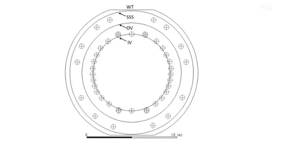
Figure 1.1. Schematic drawing of the Borexino detector

The core of the detector is the Inner Vessel (IV), a sphere of 8.4m in diameter which contains 273 tons of scintillator fluid. This liquid solution consists in PC (pseudocumene, C6H3(CH3)3) as a solvent and PPO (C15H11N O) as a solute at a

concentration of 1.5 g/l. This solution presents high scintillation yield, high light transparency and fast decay time. Pseudocumene is a hydrocarbon formed by one benzene ring and three methyl groups. PPO instead in a heteroatomic five-membered

(19)

1.1. Borexino detector

ring with two benzene rings; this benzene rings are crucial for the scintillation.

Figure 1.2. PC and PPO molecules

Inside the IV, another smaller spherical volume of 6m diameter is identified; this is not delimited by a physical boundary. The region is named Fiducial Volume (FV) and it is where neutrinos measurements are taken. Obviously this must be the purest zone of the whole detector.

The IV is made of a 125 µm thick Nylon-6 structure. Enclosing this sphere there is another Nylon-6 film (Outer Vessel) of 10.9m diameter which determines two different regions: the Inner Buffer and the Outer Buffer. The first, closer to the IV, contains 319 tons of buffer fluid. The second is filled with further 586 tons of the same fluid, a mixture of PC and few (5 g/l) DMP (dimethylphthalate, C6H4(COOCH3)2).

This solution is chemically compatible with nylon, has a low light absorption and is relatively cheap. The possibility of scintillator solution leaking outside in the buffer (and vice versa) has been considered. During the whole lifetime of the experiment a 1.5m3 of fluid exchange, in either directions, could occur. Anyway, this is not affecting the results in a relevant way [7].

In reality, after one year of experiment, a leakage was found; from a spot in the upper part of the IV a flux of 1.5m3/month towards the buffer was changing the IV spherical shape. The DMP concentration in the buffer was decreased from 5 g/l to 2 g/l so to reduce the flux. Instead, in order to restore the shape, new scintillator fluid has been inserted inside the IV in two different moments, October 2008 and June 2009 [8]. The nylon structures are so thin because the buffer and the scintillator fluids have practically identical physical properties. Densities in particular differ by one time per thousand [9]. These structures are attached with Synthetic Texitle ropes to a rigid Stainless Steel Sphere (SSS).

The SSS has the fundamental role to sustain, on its inner surface, the 2212 photo-multipliers committed to the collection of the scintillation light. All but 384 PMTs are equipped with light concentrators, designed to reject photons that are not coming from the FV. The SSS, 13.7m diameter and 8mm thick, is supported by 20 steel legs and it is fully contained by an outer tank filled by 1000 tons of high-purity water. This final layer has the role of both detecting high-energy muons passing through the SSS and decreasing the γ rays coming from the surroundings of Borexino.

Finally, on the floor beneath the SSS, two steel plates are present, an additional shielding from rocks radiation [4].

(20)

Figure 1.3. DMP molecule

More information regarding the instrumentation employed in the detector is presented in the next section 1.2.

1.2 Background stability

Borexino expects to observe 0.35 neutrino events per day per ton of scintillator liquid. Because there are so few events it is desirable to have a total background event rate that is very small; basically, solar neutrino events cannot be distinguished from background events. The rate of background events that are not identified and removed through cuts during analysis should be less than the neutrino rate. The signal to noise ratio should be S/N>1; the only way to increase this number is to reduce the background.

Enormous efforts are put into dealing with the large number of radioactive isotopes that decay with energies in or above the region of interest.

1.2.1 External background

With external background is intended all the radiation originated in the outside environment or in the material within the detector but still out of the FV. Some of the backgrounds are easily absorbed, while others, like muons, penetrate the shielding and must be subtracted from the collected data.

Ambient activity levels can vary from earth’s average. Neutron flux from the rock walls of the Hall C was measured to be 3.8n/cm2_{/s. γ flux is also present and}

almost completely absorbed by the water shield.

Muons that pass through the inner vessel produce scintillation light. Their pres-ence is a problem for Borexino even though they are efficiently tagged by the muon veto with an efficiency of better than 99.98%. Around 5000 muons per day enter the SSS and some of them interact with nuclei in the scintillator. Muons can break apart nuclei producing radioactive isotopes [6]. In this way muon-induced neutrons propagate rapidly through the scintillator but at the same time they can be detected because of the presence of a parent muon which crossed the boundary and deposited a large amount of energy [8].

(21)

1.2. Background stability

Material activity of the materials used to shield the detector is also relevant and was carefully considered in the design phase. Again, particular concern were the γ emitters. It has been not easy to measure and catalogue the impurities in every material.

Some backgrounds are also produced by PMTs and the only way to reduce their impact in the FV was to move them to larger radius and so enlarge the SSS [6]. The contribution of the light source system is approximately 1/5 of that from the PMTs in the whole scintillator volume for events above 250 keV, but it drops to about 104 of it in the 100-ton expected fiducial volume. The radioactivity of the system is thus acceptable [9].

1.2.2 Internal background

Internal backgrounds include any decay that occurs inside the fiducial volume. They are a result of the presence of radioactive isotopes in the liquid scintillator. By eliminating sources of radioactive background in the target mass the rare interactions of neutrinos will become visible.

One of the most challenging technical issues facing Borexino is the identification and elimination of the impurities in the scintillator. Anyway, there is a vast quantity of data regarding naturally occurring isotopes; the knowledge of how each isotope decays, the energies of those decays, and their half lives facilitates the identification.

The rate of background events from radioactive isotopes produced in the detector is given by the number of atoms in the detector divided by their mean life. Isotopes with mean lives much longer than the duration of the experiment will produce a background that is nearly constant in time.

Radioactive isotopes in nature are part of a decay chain. The two most common are the 238U and232Th chains. If either of these elements is present in the scintillator they will produce a series of radioactive decays that will produce a background in the detector. The concentrations of elements in the decay chains can be converted to an initial equivalent amount of 238U or 232Th. This gives a standard way of describing the concentration of all elements in the chain. However some factors can break this equilibrium. This is frequently done by the noble gas radon. Once equilibrium has been broken, describing the chain in this way is no longer valid [6].

14_C

14_{C is by far the largest Borexino background and it determines the detector low-energy}

threshold. In order to reduce the levels of contamination, the Borexino scintillator is derived from petroleum from deep underground where the levels of 14_{C are reduced}

by roughly a factor of a million compared with the usual values in organic materials. The 156 keV 14_{C end-point is low enough that it is possible to safely fit the energy}

spectrum beyond it and keep high sensitivity to the neutrinos detection.

210_Po

210_{Po is after}14_{C the most abundant component of the detected spectrum. The strong}

ionisation quenching of the scintillator brings its spectrum within the neutrinos energy region. Even though it is a direct daughter of 210_{Bi, the rate of} 210_{Po was about}

(22)

800 times higher than that of 210_{Bi at the start of data taking. Its energy region}

shows a significant non-uniformity, further perturbed by the detector operations and mixing [3]. A relevant feature which gave credence to the convective fluid movement was a low-210_{Po volume that rose from the bottom to the top of the IV between}

August and November 2014. This phenomenon can be seen as polonium falling along the periphery of the vessel and afterwards levitating through the middle of the IV. Indeed, the problem is that the combined bismuth+polonium levels have been oscillating in a non-predictable fashion even though spectra fitting has been attempted for different periods [10]. Thus, it is clear that the understanding and the prediction of the fluid-dynamic of the scintillator fluid inside the IV is a fundamental task in order to increase the detection quality of Borexino.

222_Rn

The detector exploits the nylon vessels as a barrier to prevent radon from reaching the FV. The effectiveness of the barrier is determined by the reduction of the radon concentration across a thin nylon membrane. Radon properties are typical of a noble gas, being essentially non-reactive and having a large diffusion constant making it highly mobile. Its diffusion is governed by Fick’s Law

− →

Φ = −D∇ρ (1.1)

where −→Φ is the flux, D is the diffusion constant, and ρ is the density of radon. This can be after combined with the continuity equation

∇ ·−→Φ = −∂ρ

∂t (1.2)

Finally, to be complete, a source term has to be inserted due to the radium decay, and a loss term as well due to the radon decay itself

∂ρ

∂t = D∇

2_{ρ − λ}

0ρ + ARn (1.3)

where λ0 is the decay constant of radon.

A lot of effort has been put into understanding and reducing radon contamination in Borexino. Moreover, radium embedded in steel also produces radon that can emanate from the surface [6].

Other dangerous background elements are40_K, 85_{Kr and} 39_{Ar, all β emitters [9].}

1.3 Borexino Thermal Monitoring & Management

System (BTMMS)

Beside a purification campaign thought to tackle the problem from the root, another idea has been developed in order to solve the issue concerning the fluctuations of the backgrounds mentioned in the previous section. The Borexino Collaboration decided to measure the temperature profiles inside and outside the detector, as well as thermally insulate it from the ambient temperature excursions of the Hall C. This has been done between late 2014 and the early 2016.

(23)

1.3. Borexino Thermal Monitoring & Management System (BTMMS)

1.3.1 Latitudinal Temperature Probes System (LTPS)

LTPS is designed as a vertical profile monitoring system. Its goal is to allow for a better understanding of temperature-driven background fluctuations. It is divided in three different sets of probes which have the scope of measure temperatures on two sides, south and north directions respectively.

The probes can be summarised as:

• 28 internal probes located next to the PMTs cable ports on top of the detector, from 0.5m outside the SSS, up to 0.5m inside the Outer Vessel;

• 20 external probes located on the external surface of the WT, complemented by 6 probes located in a T-shaped service tunnel under the detector;

• 6 external probes located on the upper dome of the WT, 1 inside the calibration clean-room located over Borexino, as well as several probes for exterior ambient air readings.

The output of this sensors is a voltage differential then converted by a C++ program to temperatures according to empirically-determined calibration functions. The internal sensors are easily accessible for removal, replacement or relocation.

The presence of probes specifically on the top and on the bottom is due to the existence of a positive gradient (higher temperatures on top, lower temperatures on the bottom) in Borexino; a precise knowledge of this gradient is paramount to keep good stability conditions and minimise internal currents.

Figure 1.4. LTPS probes positions. Division by phase of installation.

(24)

1.3.2 Thermal Insulation System (TIS)

TIS efficiently increases the thermal resistance of the largest boundary of Borexino, the water tank. It consists of a 20cm thick double layer of mineral wool material which covers the full surface. This material has a low conductivity value of ≈ 0.03-0.04 W/m · K.

Insulation started by the main surface, from the bottom up. Approximate > 1000m2

of detector surface were insulated, including the organ pipes through which the PMTs cables enter the tank toward the SSS.

Figure 1.5. Sample of the TIS material

1.3.3 Active Gradient Stabilisation System (AGSS)

AGSS consists of twelve independent water loop circuits made by 14mm diameter copper serpentine tubing. It was installed before covering the WT with the TIS. It is designed with the scope of avoiding possible transient, first of all the increase in thermal gradient between top and bottom, which can affect fluid stability. 3 m3_{/h of}

heated water are pumped through the tubes, from the upper part to the lowest, in order to provide constant temperatures (± 0.1◦C accurate controller) in the region of the system. This region is close to the topmost part of the detector and it is quite small compared to the total area of the tank [11].

Thanks to the operation of the AGSS and the collected data from the LTPS has been discovered that one temperature sensor is in a wrong position. In particular the probe number 4 on the south side of the detector and 0.5m outside the SSS (inside the water tank) is in a lower location. This sensor (s4) should be close to the middle plane, slightly higher, at a vertical position of 8.18m from the ground. Recently its position has been estimated around an height of 6m from the ground.

The set of probes in which s4 is contained is particularly relevant for the present work because the collected data are employed as an input for the CFD simulations, see paragraph 2.2.2. The position uncertainty of this sensor can affect the data analysis and consequently also the fluid-dynamics studies.

(25)

Chapter 2 Borexino thermal environment and

previous simulations

This chapter illustrates the thermal conditions the detector is normally facing. In addition, the only conductive and convective Computational Fluid Dynamics (CFD) models developed in the previous works are presented.

It is then shown the employment of the sensors data and their importance is underlined. Finally, after a brief consideration on the Rayleigh number range of operation for the present work, the idea of the convective Water Ring model is introduced.

2.1 Borexino thermal evolution

It is now time to introduce the thermal environment in which Borexino is inserted and focus on the application of the experimental results given by the BTMMS. It is crucial to understand the temperature trend and the asymmetries characterising the system.

The temperature of the air in the Hall C is generally oscillating during the year. This air is in contact with the exterior part of the water tank and, obviously, affects its thermal behaviour. The annual average surface temperature of the WT is con-tained in the range of 286K - 290K [11]. Such a variation influences the internal temperature of the fluids in the scintillator volume. Thanks to the probes of the LTPS it has been possible to monitor this internal temperature in precise spots, see figure 1.4. There are two main particularities which generate convective flows in the pseudoc-umene and are the cause of the internal currents mentioned in the first chapter. The first asymmetry in the detector temperature distribution is the top-bottom gradient. LTPS data taking begun in 2014, since then the gradient magnitude varied from a minimum value of ≈2.2◦C to a maximum of ≈5.2◦C, reached in July 2016. Borexino lifetime has been divided in three periods: the uninsulated period, before the TIS installation, a transient phase, during the installation and the fully-insulated period, after the work was completed. The detector inner temperature saw a rapid increase in the middle period, followed by a decrease and stabilisation once the TIS was totally located. This insulation system ensured the influence of the external air

(26)

temperature to be less effective. The first six months of the fully-insulated period showed significant stability in all areas of the detector.

The AGSS operation, started in December 2016, had the aim of maintaining the top temperature at a constant value of ≈17.5◦C, always higher than the environment condition. This way, the situation could be kept under control, avoiding de-stabilizing events for the background IV distribution.

The other important feature is the asymmetry between the North and South sides. This irregular distribution is due to the slight different external conditions each side is subjected to, to uneven temperatures as well as seasonal upsets. The temperature difference could reach values of ≈0.1◦C and it is function of the latitude. It the next sections it is possible to see how deeply this asymmetry can affect the internal fluid dynamics.

Thus, the detector temperature profile exhibits a vertical stratification. On the topmost region temperatures are more uniform, whereas in the bottom part the gradient is sharper and therefore the stratification presents more isotherms [11].

Figure 2.1. Initial temperature distribution for the IV. Picture taken from the 3D convective simulation of the IV (see below) of February 2017.

This is a particular situation of natural convection driven by really small asymme-tries. It means that every little variation in temperature BCs and every singularity of the employed model (time step, internal mesh, boundary layer) could bring to differences in the final solution.

2.2 Previous CFD models and simulations

Beside the installation of the BTMMS, in order to better understand the thermal and fluidodynamic development of the detector, several CFD models have been im-plemented. To do this, the simulation package ANSYS R FLUENTTM_{(v. 16,17 and}

(27)

2.2. Previous CFD models and simulations

19.1) has been exploited thanks to the computing resources of the CFDLab in the Energy Department of Politecnico di Milano, Bovisa.

Starting from the LTPS temperature data collected during the experiment, simula-tions has been carried out; boundary condisimula-tions (BCs) set up is explained in the next chapter. The outcome could afterwards help deciding the following directives for the operation of the AGSS. The purpose was, and remains, to ensure a higher stability in background shifting and predict its behaviour.

The simulations are basically divided in two types: only conductive and convective. The purpose of the first was to gain the precision of the model in calculating tempera-tures and heat fluxes both in the fluids and in the structempera-tures. The second, instead, were more focused on determining the fluid movements inside the IV. A lot of cases has been run with the target of checking the numerical noise, the influence of different BCs and simulating the presence of the AGSS.

A brief overview of the simulations is listed below. • Bi-dimensional only conductive simulations; • Three-dimensional only conductive simulations; • SSS convective bi-dimensional simulations;

• Water Ring and IV convective bi-dimensional simulations.

2.2.1 Rayleigh number range of operation

Before starting the convective simulations several benchmarking cases have been implemented with the scope of characterising FLUENT capability in reproducing physical well studied cases in literature [12] [13]. The idea was to reproduce a system as similar to Borexino as possible; so, this cases were studying the convective behaviour in cylindrical systems with a bi-dimensional schematization.

The temperatures were chosen to lie inside the range of Rayleigh number (Ra) concerning Borexino. This dimensionless parameter contains information about the convective/conductive nature of the fluid dynamics. Rayleigh number is usually defined as the quotient multiplying Grashof number (Gr ) and Prandtl number (Pr ):

Ra = β∆T gL

3

ν2 P r (2.1)

where β[K−1] is the thermal expansion coefficient, g[m/s2] is the gravitational field, ν[m4_/s2_{] is the kinematic viscosity, ∆T [K] is the temperature difference in the}

char-acteristic lengthscale of the system and L [m] is the charchar-acteristic lengthscale itself. P r quantifies the quotient between the momentum and thermal diffusivity.

The ∆T was chosen as the temperature upsets which cause the isotherm displacement and not the overall gradient between top and bottom; so, ∆T = 0.1K. Thus, consid-ering the radius of the IV, it results a characteristic length of L ≈ 0.17m separating each 0.1K isotherm.

Finally, taking the values of βP C ≈ 10−3K−1, νP C ≈ 7· 10−7m4/s2 and P r =

7.78, Rayleigh number range for Borexino application has been estimated Ra ∈

(28)

[O(107_{), O(10}8_{)]. Keeping in mind that we are not really working with a}

linearly-stratified fluid, this range has to be enlarged to Ra ∈ [O(106), O(109)].

It is important to underline that from this brief calculation it is possible to infer that the system presents a situation of laminar flow in natural convection. This is extremely important for determining a suitable model setup and the software options.

2.2.2 Water Ring

and IV convective bi-dimensional

simula-tions

The coupled bi-dimensional convective simulations of the Water Ring (WR) and the Inner Vessel are particularly significant because they represent the connection between previous works and the present.

This section is thought to give an explanation of the principal of operation of the Water Ring model; the various IV models are deeply and carefully treated in the next chapters.

The main target of the WR model is to propagate and faithfully reproduce the BCs in the inner part of the detector. These BCs are built up from the LTPS data through an interpolation process; it is clear that these temperatures are varying in time during the simulated period, usually one month.

The mesh itself presents two fluid regions, one for water and the other for the internal pseudocumene. Moreover, all the real surfaces dividing the fluids and described in section 1.1.2 are modelled.

Figure 2.2. Water Ring model structure.

It has been proved that Water Ring model is a valid benchmark for the thermal transport and quite faithful for the temperature evolution [11]. The output data have been compared to the LTPS probes inside the Outer Buffer and the difference in temperatures is less than ±0.2◦C. Anyway, the model is not a benchmark for the fluid

(29)

2.2. Previous CFD models and simulations

transport. It produces unrealistic currents or fully numerical flow patterns. This is the reason why a separate IV model is needed in order to study and characterise the internal fluid dynamics.

Thus, as a result of the WR simulation, it is possible to extract the temperatures from previously located spots at the border of the Inner Vessel (see figure 2.2). These values are consequently employed as BCs for the IV models. From the previous works, the bi-dimensional modelling of the Inner Vessel revealed stratified horizontal flows in the internal bulk. This behaviour will be confirmed by the present study.

No heat transfer on the structures is computed since the physical boundaries are modelled with zero-thickness. The walls simply represent a division between the various inner regions of the detector. While the SSS is in contact with water and pseudocumene at its borders, the other nylon films are only surrounded by scintillator fluid.

(30)

(31)

Chapter 3 Governing equations for the

mathematical models

In this third and short chapter the set of governing equation which mathematically characterises the problem is given.

In the first part is explained how the fluid-dynamic behaviour is treated. This model is afterwards implemented in FLUENT.

In the second section instead, it is described the equation used to predict the Polonium mass transfer in COMSOL Multiphysics.

3.1 Pseudocumene fluid-dynamic model

The chosen way to describe the flow field of the pseudocumene inside the IV are the mass, momentum and energy conservation equations (Navier-Stokes equations) for an incompressible Newtonian fluid. Viscosity and density are generally considered constant.

The system of equations takes the form: ∂ρ ∂t + ∇ · (ρu) = 0 (3.1) ∂(ρu) ∂t + ∇ · (ρuu) = −∇p + ∇ · τ + ρg (3.2) ∂(ρE) ∂t + ∇ · [(ρE + p)u] = ∇ · [(τ · u) + k∇T ] (3.3) Where ρ, u and E are the density, the velocity vector and the energy, respectively. p is the static pressure, ρg the gravitational body force, k the thermal conductivity and τ the stress tensor.

The basic idea of these transport equations is to have the rate of change term and the convective term on the left and the diffusive and source term on the right-hand side. The resolution method and the chosen property values are presented in the following chapter.

(32)

3.1.1 Boussinesq approximation

An important approximation has to be inserted since the problem is concerning natural convection. The Boussinesq approximation models the fluid density as a function of temperature. So, the fluid density is considered as variable in the body force term and is here linearized. This can only be done when the density variations are small.

ρg = (ρ − ρ0)g ' −ρ0β(T − T0)g (3.4)

β = −1 ρ(

∂ρ

∂T)p (3.5)

where β is the thermal expansion coefficient.

In this way it is possible to reduce the non-linearity of the governing equations. From a computational point of view, this kind of treatment provides faster convergence in respect to other temperature-dependent density formulations [14].

Easy to notice that the momentum and energy conservation equations (eq. 3.2 and 3.3) are strictly correlated by the temperature. Temperature asymmetries, in natural convection problems, are in fact the driving force of the fluid motion.

3.2

210

Po mass transfer model

The polonium migration inside the Inner Vessel is modelled through a convection-diffusion equation. The model predicts only the 210_{Po transfer, avoiding to consider}

its predictors (bismuth and lead). These other elements are considered much less mobile compared to the polonium and they cannot easily pass the nylon structure of the IV [15].

∂CP o

∂t + u∇CP o= ∇ · (D∇CP o) − λP oCP o (3.6) Where CP o is the polonium concentration, D its diffusion coefficient, λP o the decay

constant and u is the velocity vector. This vector is directly taken from the resolution of the Navier-Stokes equations previously mentioned. In such a way, it is possible to decouple the fluid-dynamic problem from the 210_{Po transfer.}

(33)

Chapter 4 2D and 3D numerical domains and

models setup

In this forth chapter it is presented in detail the the structure of the CFD models pre-viously mentioned. The target is to describe the whole numerical model development for the system.

Starting from the meshes description for the 2D and 3D cases, all the differences will be highlighted. Consequently, it is described the BCs formation procedure, from the LTPS data to the used interpolation. Furthermore, the chosen numerical model is shown. Finally, a brief paragraph on the 2D mass transfer model in COMSOL for the

210_{Po prediction is present.}

4.1 Mesh generation and geometrical model

descrip-tion

4.1.1 2D computational grids

It is important to underline that the 2D grid generation has been carried out in previous works. So, this section aspires to simply describe the taken choices.

The 2D model exhibits different geometrical simplifications in order to reduce the computational cost and time and to decrease the real number of elements of the detector. With this perspective, Borexino is designed as several concentric cylindrical domains (fig. 2.2).

The bi-dimensional computational grid used to discretize the domain is, depending by the precise position, a structured Cartesian or a polygonal/polyhedral grid. Prelimi-nary mesh sensitivity analysis permitted to determine the mesh size ∆x suitable for each geometry.

The Water Ring model, mentioned in section 2.2.2, presents a coarser discretization because its only aim is to reproduce the temperature map at the border of the IV. This particular model is composed by ≈118k hexahedral orthogonal cells with local refinements close to the walls [15].

(34)

and reliable characterisation of the internal fluid currents. Two different grids are employed for the analysis in the present work. The detailed information about the grids are stored below in table 4.1.

The usage of two distinct meshes gives the possibility to compare the obtained results and to gain some feedback concerning the differences between the two.

N◦ cells Average cell size [m] BL thickness [m] Min orthogonal quality

270k 0.01447 - 0.2727

530k 0.01034 0.020 0.6905

Table 4.1. Geometrical parameters of the 2D computational grids.

The grids have a number of cells in the order of O(105_{). Easy to understand that}

the attempt is to double the cells between one case and the other.

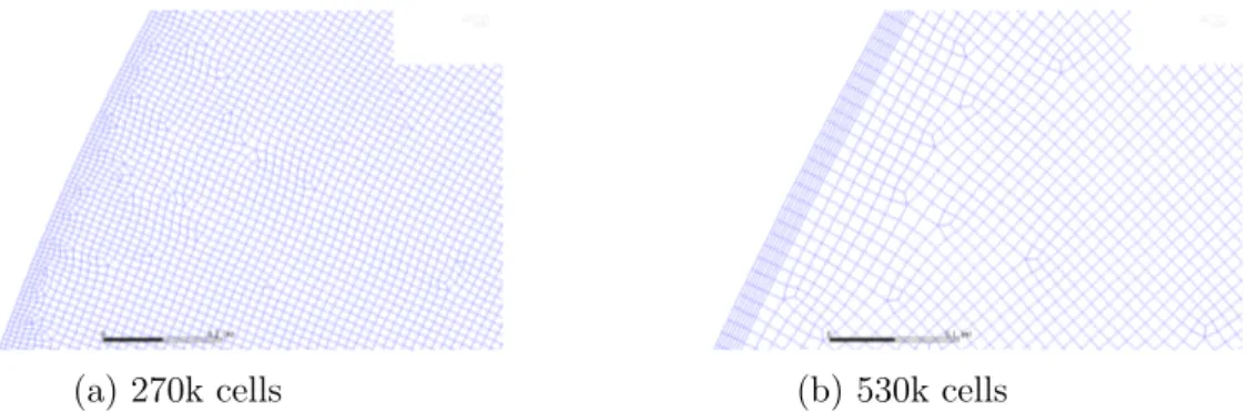
The average cell size is simply obtained dividing the area to the number of cells. It can be also seen that the first mesh is characterised by an acceptable value of orthogonal quality while the second reaches a good one. Moreover, some observations should be done about the boundary layer thickness. With boundary layer thickness it is intended the length of all the layers of cells present at the border of the domain. These layers are intentionally structured to better compute the boundary thermo-fluid dynamic trend. It can be noticed that in the 270k cells mesh such a solution is not present (fig. 4.1a); it has been opted just for a local refinement. In the other mesh there are seven organised layers (fig. 4.1b) and their thickness amounts to 2cm; this choice turned out to be healthy for the behaviour understanding.

(a) 270k cells (b) 530k cells Figure 4.1. Boundary layer comparison for the 2D cases.

4.1.2 3D computational grids

Differently from the 2D cases the generation of the 3D meshes have been developed in the present work. For this particular task has been always exploited the FLUENT package, in particular the FLUENT 3D meshing option.

The generation process started from a very simple sphere CAD model. This sphere has a diameter of 8.5m in order to reproduce the real dimensions of the IV. Once the CAD was imported it has been possible to define the minimum and maximum

(35)

4.1. Mesh generation and geometrical model description

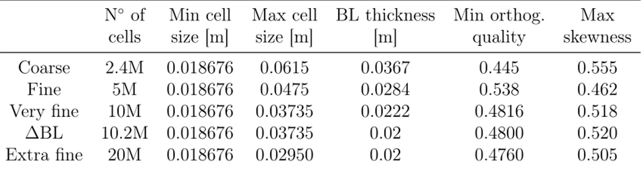
cell size and the number of layers of the BL for each case. At the variation of the maximum cell size a different number of cells has been reached. All the geometrical parameters are summarised in table 4.2.

N◦ of Min cell Max cell BL thickness Min orthog. Max

cells size [m] size [m] [m] quality skewness

Coarse 2.4M 0.018676 0.0615 0.0367 0.445 0.555

Fine 5M 0.018676 0.0475 0.0284 0.538 0.462

Very fine 10M 0.018676 0.03735 0.0222 0.4816 0.518

∆BL 10.2M 0.018676 0.03735 0.02 0.4800 0.520

Extra fine 20M 0.018676 0.02950 0.02 0.4760 0.505

Table 4.2. Geometrical parameters of the 3D computational grids.

Again, the idea is to every time double the number of cells in order to have a comparison and to understand, through a sensitivity analysis, when the discretization is good enough. The number of elements is in the order of O(106). All the meshes have tridimensional polyhedral cells in the whole volume except for the external layers. Both values for orthogonal quality and skewness result acceptable in each case. The grids have been generated in two different moments along the project evolution. At first, the three smallest meshes were built up; in a second moment, the generation has been completed with the addition of the biggest two. The substantial difference between the two groups is the BL structure. While in the fist case only the number of layers (6) has been imposed, in the second the intention was to reproduce in 3D the bi-dimensional layout which brought to satisfying results (see chapter 5). So, the 10.2M and 20M cells grids boast the presence of 7 layers with the smallest total thickness of 2cm. The BL thicknesses of the other specific cases are reported in table 4.2. The comparison can be appreciated in the figure below.

(a) 2.4 Millions of cells (b) 10.2 Millions of cells Figure 4.2. Boundary layer meshes comparison.

The Z axis of the model is associated to the vertical one. The image compares the meshes from the views of the ZX vertical plane. The difference in dimensions is clear.

(36)

4.2 Initial and boundary conditions

It is now described how the data from LTPS are treated in order to generate the initial and the boundary conditions for the different cases. Some differences are present between the 2D and the 3D domains so they will be discussed separately.

The idea is to linearly interpolate the known values located in the precise positions. Doing that, we are assuming a smooth behaviour between the various spots.

It is essential to underline that the Water Ring simulation (section 2.2.2) is only computed in two dimensions. The output temperatures taken from thirty spots at the border of the Inner Vessel are later employed for generating the BCs of both the 2D and 3D only IV models.

4.2.1 Bi-dimensional case

The initial conditions are imposed through a linear interpolation. The domain is practically divided in rectangular sub-domains who’s vertices are identified by the imposed temperature spots. The initial temperatures for all the points inside the smallest domains, with coordinates (x,y), are given by the interpolation function:

T (x, y) = 1

A[(∆T (R1) · |x − x0| + ∆T (R0) · |x − x1|)y+ +|x − x0| · (T1y1− T2y0) + |x − x1| · (T4y1 − T3y0)]

(4.1)

where A is the area of the rectangle, Ti, with i = 1, 2, 3, 4, are the temperatures of the

vertices and R0/1 are the vertical temperature gradients between the north and the

south vertices respectively.

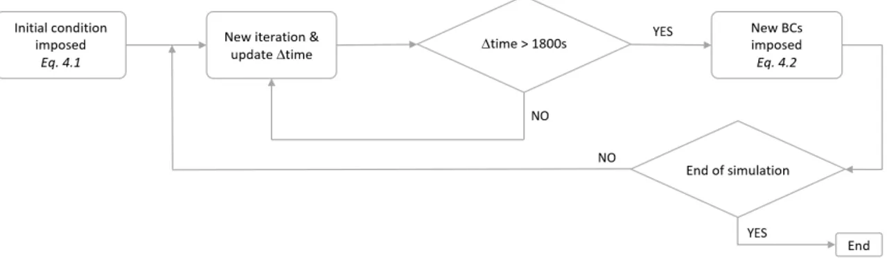
As the simulation proceeds in time, updated boundary conditions have to be provided.

Figure 4.3. Simplified flow chart of the BCs imposition.

Every 1800s of the simulated time, which is the standard time delay for the LTPS data acquisition, new temperatures are given at the border. To do this, the simulated time is constantly monitored through a loop; in the schematic flow chart ∆time represents the period passed after new conditions are given. Also in this case a linear

(37)

4.2. Initial and boundary conditions

interpolation is exploited to guarantee a full and continuous profile in the boundary points. The temperatures are now function of time and the vertical position:

TN/S(t, y) =

1 hi

1− hi0

[T_N/Si+1(t) · (y − hi₀) + T_N/Si (t) · (hi₁− y)] (4.2) where h0/1 are the heights of two adjacent known spots, i∈ [1,14] is the corresponding

domain and N/S is the side.

This custom-made function (time-evo), which is internally developed by the Borexino collaboration, was verified to not generate deep enough changes to cause numerical divergences. For this reason it is also used for the tri-dimensional model.

4.2.2 Tri-dimensional case

In the 3D case it is not possible anymore to only execute a simple linear interpolation, the sub-domains are not rectangles but they have an unstructured shape.

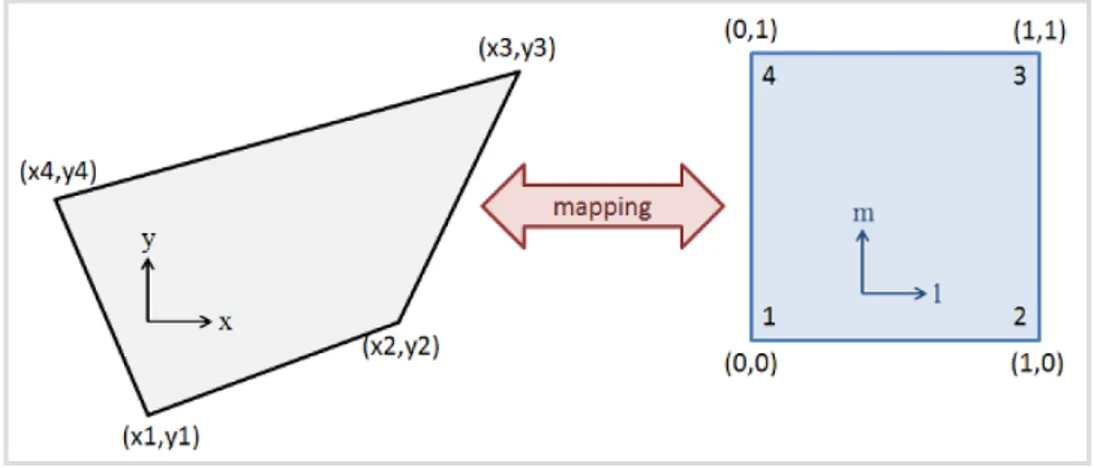
The procedure consists in the formation of a mapping function able to transform an arbitrary quadrilateral into a square. This function will pass from physical to logical coordinates (x, y) = f (l.m) where both l and m ∈ [0, 1]. In this way it is possible, and even in an easier way, to implement a linear interpolation [16].

Figure 4.4. Mapping function schematic behaviour.

It is interesting to notice that, even if the result is a 3D temperature distribution, the interpolation anyway starts from bi-dimensional data; this is due to the location of the available LTPS probes, only present in the north and south sides. So, once the interpolation is done in two dimensions, the temperature pattern is applied both to the west and east 3D semi-spherical surfaces, in a fully symmetric way.

The mapping function is modelled as a bi-linear system:

x = α1 + α2l + α3m + α4lm (4.3)

y = β1+ β2l + β3m + β4lm (4.4)

Where the alphas and the betas, 4 for each domain, are obtained through the resolution of linear systems. These indices contain the information for every map to pass from physical to logical coordinates, and vice-versa.

(38)

Later, l is found inverting equation 4.3 and m from the consequently quadratic equation obtained from equation 4.4.

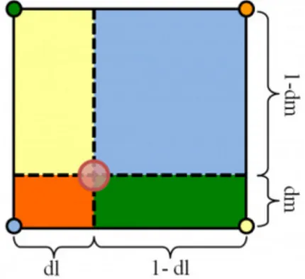
Figure 4.5. Area division for the linear interpolation in logical coordinates.

Since the area in logical coordinates is unity, temperature inside the domain is given simply by the sum of the vertices temperatures times the opposite area, see figure 4.5 for a better understanding.

T (m, l) = T1(1 − m)(1 − l) + T2l(1 − m) + T3ml + T4m(1 − l) (4.5)

The boundary conditions are always imposed thanks to the time-evo function. The flow chart seen in figure 4.3 is still valid. In this case the interpolation just explained is inserted in the function, eq. 4.2 is substituted by eq. 4.5. Also the alphas and the betas have to be added at the beginning. Clearly, the conditions are given in three dimensions.

4.3 Numerical model setup

The mathematical model presented in chapter 3 is implemented in the commercial software ANSYS FLUENT through a discretization in space and time.

4.3.1 Numerical algorithm

The algorithm employed for the equations resolutions is the coupling pressure-velocity PISO algorithm, which stands for Pressure Implicit with Splitting of Operations. It has been originally implemented as a non-iterative transient calculation procedure. With non-iterative is intended that it does not require iterations within a time level. Once the solution is reached inside the PISO process it is possible to pass directly at the following time step. To ensure good and accurate results a small time-step is required.

The PISO process presents internal loops and it can be considered as an extension of the SIMPLE method because it contains a further pressure correction equation. For this reason, an additional storage is asked but with the result of an efficient and faster method [17].

(39)

4.3. Numerical model setup

4.3.2 Discretization schemes

The discretization scheme is equally employed in 2D and 3D. In the tables below are reported the chosen solution methods.

Term Scheme

Gradient Least squares cell based Pressure Body force weighted Momentum, Energy Third order MUSCL Transient First order implicit

Table 4.3. Numerical discretization schemes.

As said, it is here evident that PISO is a transient implicit method. The choice of third order MUSCL scheme for momentum and energy equations grantees a highly accurate numerical solution.

To control the convergence and get a more stable solution some under-relaxation factors are set. All the other factors are fixed to one.

Correction Factor Pressure 0.3

Momentum 0.7

Table 4.4. Under-relaxation factors.

4.3.3 Time-step definition

The time-step (∆t) has been chosen in order to maintain the necessary accuracy and to satisfy the Courant-Friedrichs-Lewy (CFL) condition of CFL<1. ∆t is defined considering the physical ∆Tp and the Fourier stability analysis.

∆tp = τ0 4 ≈ L 4pβgL∆Tp (4.6) ∆tF o = F o(∆x)2 α (4.7)

with τ0 the time constant, L the characteristic length, F o the Fourier number limited

to F o = 0.1, ∆x the grid size and α = k/(ρcp) the numerical diffusivity. The maximum

time-step for the different cases has been chosen [11]. The starting values for the 2D and 3D cases were 4.5s and 9s respectively. Considering that the simulated time is around 4 weeks, several hundreds of thousands of time-steps are needed.

(40)

Density ρ 881 [kg/m3_]

Viscosity µ 1.112·10−3 [Kg/(m· s)] Thermal expansion coeff. β 1.05·10−3 [K−1]

Table 4.5. Fixed properties for the pseudocumene.

4.3.4 Physical and thermal properties

The physical and thermal properties of the pseudocumene are listed in table 4.5. These are the values inserted in the model:

Density is specified at operating temperature of 288K. Viscosity is considered constant. The value for fluid thermal expansion coefficient β, which enter in the Boussinesq approximation, has been previously derived by density measurements at different temperatures.

The heat capacity and the thermal conductivity are instead given by user-define temperature dependent polynomial functions:

cp = 1497.075 − 1.14419T + 0.00713T2 (4.8)

k = 0.203 − 2.72 · 10−4T + 8.52 · 10−8T2 (4.9) Additionally, the default values for all the interested water properties in the WR simulation are taken.

4.4

210

Po mass transfer model

The mathematical model presented in section 3.2 has been implemented in the com-mercial software COMSOL Multiphysics. This model can give a prediction of the

210_{Po concentration inside the FV which can be compared with the experimental}

measurements.

The model contains several simplifications.

For the bi-dimensional cases the spatial discretization is taken equal to the FLUENT simulations. For the 3D model instead, a new less refined mesh with 1.1M of tetrahedral elements is directly crated in COMSOL.

The velocity field is taken from the CFD simulations. The velocity values are interpolated by the new software. Anyway, the mass transfer simulation setup maintains a constant velocity over time; this is giving reliable results since the temperatures at the border are experiencing very small variations and the situation is considered stable. The final solution can be considered as a picture of a 210Po concentration evolution at a specific time.

The boundary conditions for the polonium concentration are then set and imposed to the equation 3.6. The concentration is assumed to be constant and uniform over the IV wall. Such a distribution comes from the idea that polonium uniformly migrates through the nylon film all around the vessel.

(41)

Chapter 5 Results of the 2D cases

The results, the computed analysis and the considerations about the various models are now presented. First, the 2D results are shown; consequently, another chapter about the 3D cases is inserted. Both parts contain a description of the fluid-dynamics and the results evolution; finally, an analysis of the 210Po distribution prediction is added.

The simulated time is around 1 month, precisely 2’584’800s. The exploited LTPS data are related to the last week of January 2017 and the first three of February 2017. In the 2D case the total duration of the simulations (WR + IV model) is around 2 and a half weeks.

The main target of the 2D simulations is to characterise the fluid-dynamics of the IV pseudocumene and extract the velocity field. Beside this, a part of the investigation is focused on the problem with the unknown position of the temperature sensor s4, see section 1.3.2; two different temperature interpolations have been defined for the Water Ring simulation in order to impose the right profile. A complete list of the 2D

analysis is now given:

• Comparison between the outputs of the three WR simulations: base case, 1◦

and 2◦ interpolation;

• study and comparison of the velocity field, output of the IV simulations with the coarse mesh: base case, 1◦ and 2◦ interpolation;

• study and comparison of the velocity field, output of the IV simulations with the fine mesh: only base case and 2◦ interpolation;

• overall analysis of the 210_{Po distribution prediction.}

So, the chapter is divided in three parts. First of all, the WR section. Second, the cell size sensitivity analysis on the IV model. Finally, the polonium distribution prediction.

5.1 Water Ring simulations

The WR simulation is the first step of the bi-dimensional analysis. Since the LTPS data of the probes 0.5m outside the SSS are employed as BCs, the set of probes

(42)

situated 0.5m inside the SSS are exploited as a comparative benchmark for the simulation outputs. From the results, temperature data are extrapolated in the exact position of the internal probes and the values are compared.

The procedure has been followed for three different cases:

• In the base case, the BCs are taken from the LTPS data without changes. s4 is thought to be at 8.18m from the ground;

• for the first interpolation, the value of the s4 temperature in the BCs has been linearly interpolated between the two adjacent probes. Its position is always assumed at 8.18m from the ground, as designed;

• in the second interpolation the vertical position of s4 has been set to be 6.28m from the ground and its value has been again linearly interpolated.

The simulations of the base case and the second interpolation have been carried out by Eng. Valentino Di Marcello (INFN) while the first interpolation and the whole post processing have been produced by the author of the present work.

(a) Base case. (b) 1◦ interpolation.

(c) 2◦ interpolation.

Figure 5.1. Water Ring simulation accuracy check – South side.

Attention has to be payed; the sensors reported in the figures are the internal ones. As said above, the simulation data are compared with the experimental data recorded in the same positions, which are represented by the thinner lines. To avoid

(43)

5.1. Water Ring simulations

misunderstandings, from now on, the names of these internal probes are written in bold-italics.

Looking at the figures it is clear that in the base case the temperatures are well reproduced in the upper part of the detector (s1-s2-s3 ) and weakly overestimated or underestimated, with an error which is around 0.15◦C, in the lower area.

With the first interpolation the value of temperature in s4 has clearly increased. The behaviour is consistent with the physics of the system because we are assuming for the external s4 a position that is higher than the real one. The topmost part always shows higher temperatures even if the temperature gradient is decreasing from the bottom to the top. This change has a repercussion also on the values of the probes s5 and s6 ; for these two the match with the data is improved. It is possible to infer that this would have an impact on the fluid-dynamics of a consistent part of the vessel.

Finally, with the second interpolation the situation seems to be very similar to the base case. In fact, the external s4 is now assumed to be closer to its real position. Small variations from the experimental data are anyway present.

(a) Base case. (b) 1◦ interpolation.

(c) 2◦ interpolation.

Figure 5.2. Water Ring simulation accuracy check – North side.

When it comes to the north side the trend is similar to the south side. Initially, a good reproduction is found for the bottom are; some irregularities are instead noticed in the other sensors, specifically for the internal n5 .

From figure 5.2b it is possible to see how all the probes reach a higher temperature. The reason is the same of the south side situation. Here probably, the perturbation is

(44)

less strong than the previous case, but visible at every height.

In conclusion, the second interpolation still brings the results close to the base case. Having seen these differences between the various WR model cases, it is now possible to introduce the results of the IV model simulations.

5.2 Cell size sensitivity analysis

Two models are studied in this paragraph. The goal is to appreciate the differences and pay attention on the resolutions of the results. First of all, a coarse computational grid is employed, with 270k cells. Afterwards, a refined mesh is exploited, the one with 530k cells. For each case, the mentioned BCs, outputs of the WR model, are imposed.

5.2.1 Coarse computational grid

This section contains the results of the first IV model, with a computational grid of 270k cells. The comparison is always done between the base case and the two interpolations, as explained right above. The main differences will be highlighted.

In order to characterise the evolution from the beginning, a strict monitoring of the velocities has been computed. This is the only analysis carried out for the base case solely. 21 points have been created in order to extract the velocity magnitudes, see figure 5.3b. For the first part of the simulation, every 1000s data has been saved. The result can be seen in the following image.

(a) Initial velocity magnitude evolution – Base case. (b) Monitoring points. Figure 5.3

The velocities, starting from a default value of 1 · 10−10 m/s, rapidly increase and reach a peak after approximately 1000s of simulations. The initial order of magnitude is O(10−3) m/s. Thus, the trend shows a fast decrease until a stable situation is found around 20000s (≈ 6 hours). Small fluctuations are continuously present. The behaviour is comparable for the majority of the points.

(45)

5.2. Cell size sensitivity analysis

The temperature distribution confirms the isotherms stratification mentioned in chapter 2. The evolution is consistent with the imposed BCs. Temperatures are slowly changing at every height of the vessel. For instance, fixed the vertical coordinate at Y =5.85m, on that line the temperature sees a change of 0.0108◦C/day. The situation is quite stable.

After the initial transient period shown in figure 5.3a, the magnitudes remain con-stant and the velocity conformation is stable. For this reason it is below reported only the situation in a single instant, in particular after 1’836’000s (≈ 21 days) of simulation.

The velocity magnitude distribution is shown in figure 5.4.

The final order of magnitude which is computed by this simulation is O(10−5) m/s.

Figure 5.4. Velocity magnitude. From the left: base case, 1◦ and 2◦ interpolation.

It is possible to notice a higher velocity region in the bottom part of the IV with a clear motion stratification. In the central part, a peculiar leaf-shaped conformation is visible in the three cases. This is associated to numerical noise caused by a poor grid refinement. Finally, in the very bottom part, another nonphysical solution is present; this is again due to the grid.

The two interpolations generally reveal a lower velocity except for a thin layer close to the top. These are the expected effects generated by the small change in the BCs. The change is visible in the whole vessel; it is an evidence of how much sensitive the Borexino fluid-dynamics is.

More details on the effective inner motion are given by the horizontal velocity. The fluid shows a horizontal stratification in all the domain. This is absolutely

Figure 5.5. Horizontal velocities. From the left: base case, 1◦ and 2◦ interpolation.

confirming the results of the previous works. So, the model is telling us the vessel

CFD modelling of the Borexino solar neutrino detector : investigation of the inner vessel fluid-dynamics and polonium concentration

Politecnico di Milano