level of landslide susceptibility zoning of the area, developed on the base of nowadays available data, on which more sophisticated studies can be developed.
Keywords: debris flow, susceptibility descriptors, rheological law, numerical analyses, susceptibility zoning
Introduction
Debris flows are very rapid to extremely rapid surging flows of saturated debris in steep channels with strong entrainment of material and water from the flow path [HUNGR et al., 2001, 2014; JACOB et al.,
2005]. They are distinct from other types of landsli-des because they occur periodically on established channels, usually gullies and first- or second order drainage channels. Thus, debris flow hazard is spe-cific to a given path and deposition area (“debris fan”). The above aspects, and the periodicity of oc-currence at the same location, influence the metho-dology of hazard studies [HUNGR et al., 2001, 2014;
JACOB et al., 2005].
An important part of any landslide hazard or risk assessment is the quantitative estimate of post-failu-re motion (“runout”) including travel distance, flow height and flow velocity. Several approaches have be-en developed to model fast gravitational mass mo-vements in order to assess their characteristics, in-tensities and run out. The available methods give a good systematic approach to assessing the sprea-ding, extension and impact that a landslide can ge-nerate. These methods can be divided into empiri-cal, analytical and numerical methods. A good over-view of methods for run-out modeling is given by HÜRLIMANN et al. [2008] and HUNGR [2016].
In particular, numerical models are based on fluid mechanics and solve the equations of mass and momentum conservation numerically after discreti-zing them in both space and time. The stresses in the momentum conservation equation are
determi-ned from the assumed constitutive law of the flowing material. Most models are based on a “continuum approach” that considers the loose, unsorted and multiphase material of a landslide as a continuum [PASTOR et al., 2012].
The depth-averaged shallow water equation ap-proach using different solvers has been applied com-monly for numerical simulations of rapid mass mo-vements over complex topographies [CROSTA et al.,
2006; PASTOR et al., 2009]. Depth averaging allows
re-presenting the rheology of the flow as a single term that expresses the frictional forces that act at the in-terface between the flow and the channel bed.
In the framework of the continuum and discon-tinuum methods, the depth-integrated SPH method proposed by PASTOR et al. [2009] is particularly
suita-ble for analysing landslides that have average depths which are small in comparison with their length or width. The mathematical model of SPH method pro-posed by PASTOR et al. [2009] is based on v-pw Biot-
Zienkiewicz model. Assuming that for flow-like lan-dslides the average depths are small if compared with their length or width, it is possible to simplify the 3D propagation model described above by inte-grating its equations along the vertical axis. In this way, the Biot-Zienkiewicz equations for non-linear materials and large deformation problems are cou-pled to various constitutive models (Bingham, Voel-lmy, Mohr-Coulomb, etc.), obtaining a 2D depth-in-tegrated model, which presents an excellent combi-nation of accuracy and simplicity and provides infor-mation about propagation, such as average velocity or depth of the flow along the path.
The numerical model used for the mathema-tical problem’s resolution is the smoothed particle hydrodynamics method (SPH). The SPH model is a mesh-free method that provides an interesting and
* Department of Civil, Energy, Environmental and Materials Engineering, “Mediterranea” University of Reggio Calabria, Italy
48 MORACI - MANDAGLIO - GIOFFRÈ - PITASI
powerful alternative to more classical numerical me-thods such as the finite elements method.
Smoothed particle hydrodynamics is based on discretized forms of integral approximations of fun-ctions and derivatives. The SPH method introduces the concept of ‘particles’, to which information con-cerning field variables and their derivatives is linked. In particular, smoothed particle hydrodynamics me-thod is based on the possibility of approximating a given function f(x) and its spatial derivatives by in-tegral approximations defined in terms of a kernel. In a second step these integral representations are numerically approximated by a class of numerical in-tegration based on a set of discrete points or nodes, without having to define any “element”.
In order to simulate entrainment of material from the path, PIRULLI and PASTOR [2012] have
for-mulated several algorithms. A number of much mo-re sophisticated solutions have appeamo-red in mo-recent years, based on treating the fluid and solid phases of the flow separately using mixture theory (e.g. IVERSON
and GEORGE, 2014).
The study of post-failure motion (“runout”) in-cluding travel distance, flow height and flow veloci-ty enables to obtain a spatial prediction for landsli-des and it contributes significantly in the landslide susceptibility mapping inside the framework of risk assessment (e.g. LEE et al., 2004; HUNGR et al., 2005;
FELL et al., 2008a). The susceptibility maps assist
plan-ners, local administrations, and decision makers in disaster planning. Among the approaches available in literature, the term “susceptibility” does not assu-me the saassu-me assu-meaning. In the paper, the susceptibi-lity has been considered, according to the approach of FELL et al. [2008a], as a quantitative or
qualitati-ve assessment of the classification, volume (or area) and spatial distribution of landslides which exist or potentially may occur in an area. Susceptibility may also include a description of the velocity and intensi-ty of the existing or potential landslides. Although it is expected that landslides will occur more
frequen-tly in the most susceptible areas, in the susceptibility analysis, the time in which landslides have occurred is not taken into account. It has been taken into ac-count in the landslide hazard considering the return period.
In the paper, the susceptibility has been conside-red as spatial probability of occurrence but not tem-poral (hazard), and the susceptibility analyses have been based on two assumptions that the past is a gui-de to the future, so that areas which have experien-ced landsliding in the past are likely to experience landsliding in the future and that the areas with simi-lar topography, geology and geomorphology as the areas which have experienced landsliding in the past are also likely to experience landsliding in the future.
This paper shows a mixed approach to obtain su-sceptibility maps in an area located between Scilla and Favazzina (Reggio Calabria), which has been re-currently interested by rainfall-induced debris flows [GULLÀ et al., 2005, 2006; MANDAGLIO et al., 2016].
The source areas of the landslides have been pre-dicted using an heuristic method based on available data (observed phenomena and on geological/geo-morphological setting of the area). For this purpose, detailed and validated in field thematic maps have been used. The propagation phase of debris flows has been analysed by an advanced numerical model to assess the path, the travel distance and the velocity of flowing mass.
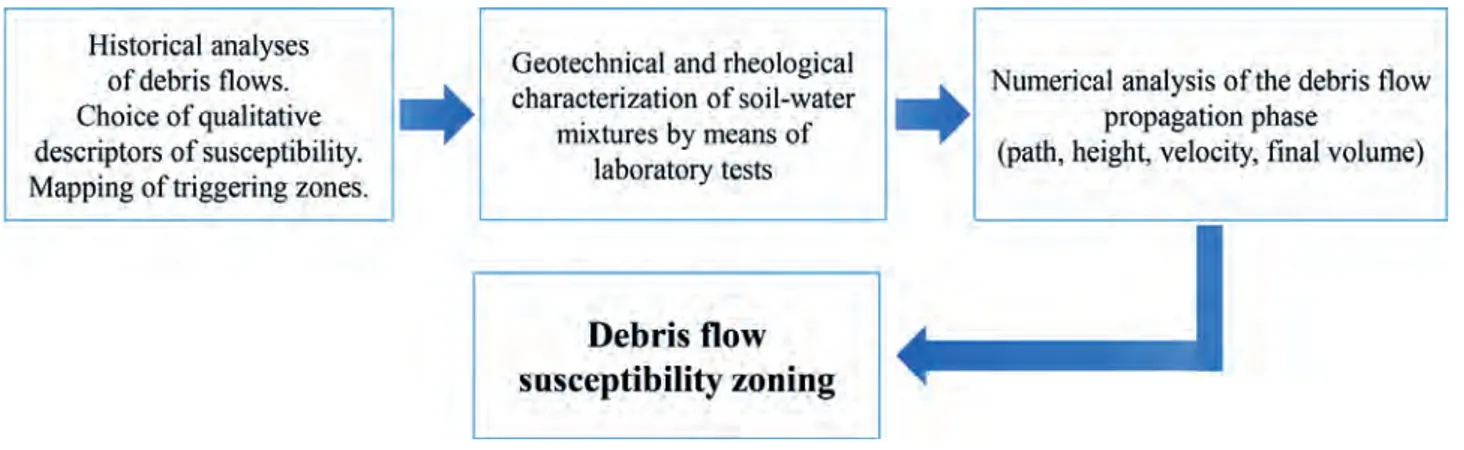
The proposed approach is summarized in the flow chart shown in figure 1, and it is composed by four stages:
a. Debris flow inventory mapping and prediction of source areas. Historical analyses of past debris flows have been performed in order to obtain the susceptibility descriptors. Therefore, predicted triggering zones have been identified taking into account areas with susceptibility descriptors like those of the past events. The results of this stage have been the base for the identification of areas where potential debris flows could occur.
Fig. 1 – Flow chart of the proposed approach.
Study Area
In the present research, the tested area is a zo-ne located between Scilla and Favazzina (Reggio Ca-labria, Italy), affected by several events of recurrent debris flow landslides. These events propagate in “V” shaped channels and, along them, material is entrai-ned and large amount of water is available which cau-ses the propagating mass to fluidize, even without li-quefaction has occurred in landslide source areas.
The zone falls within an extremely complex area characterized by the presence of several tectonic structures, frequently intersected each other, cros-sing the rock masses belonging to the crystalline me-tamorphic basement of Aspromonte. The crystalli-ne-metamorphic bedrock of the area is constituted by continental crust of the Aspromonte- Peloritani Unit, of Hercynian age [PEZZINO et al., 1990; BORRELLI
et al., 2012], formed by a migmatitic complex intru-ded by granites which are alternated to biotitic para-gneiss, often with traces of partial melting and mig-matitic gneiss with high biotitic concentrations.
Referring to the test area, the main lithologies that typically outcrop are residual soils (reddish-brown silty-sandy blankets encapsulating very wea-thered rock fragments) that cover a crystalline be-drock. The slope stability conditions of the area are strongly controlled by the weathering degree of the rock masses [GULLÀ et al., 2005; 2006], by the climatic
conditions as well as by tectonic and geomorphic fac-tors. Shallow landslides generally occur during the wet season and quickly evolve, following mechanisms classified as debris flows. The flows occurred perio-dically in steep channels with strong entrainments of material and water from the whole flow path.
The most part of sediments that form the coast were originated by such processes.
From the hydraulic point of view, it must be pointed out the strong erosive and transport capa-city of the streams (e.g. Favazzina, Favagreca, Scirò, Condoleo, Prajalonga, Mancusi, Rustico) that is able to transport disruptive amount of water and debris [MANDAGLIO et al., 2015; 2016].
a single information system for the landslides in Italy and the homogenization of the national data. Moreo-ver, additional information available in literature on a real event have been used [BONAVINA et al., 2005].
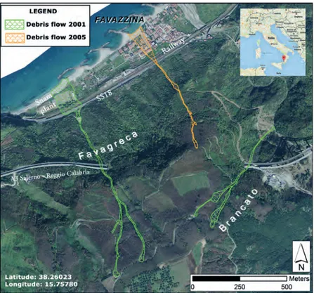
Past events in the area occurred in 2001 and in 2005 producing extensive damage which involved va-rious lifelines as shown in figure 2. Particularly, on 12 May 2001, debris flows were triggered by heavy rainfalls at the head of the Favagreca channel, re-spectively at 600 and 610 m above sea level in corre-spondence of two stream incisions which converge at about 400 m a.s.l. The debris flow runout hit the SNAM station of the methane pipeline, the main ro-ad SS 18 and the railway causing the derailment of the intercity train Turin - Reggio Calabria. Available studies [BONAVINA et al., 2005] have shown that the
volumes at the end of the propagation were tripled respect to trigger one (Vi ≅ 1.130 m3) in the 2001
event. During the same event, a second debris flow, in an adjacent valley, has invested the A3 - Salerno Reggio Calabria at the Brancato tunnel. This debris flow has not been considered in the paper because the runout was outside the examined area.
On 31 March 2005, another debris flow activated on the slope overlooking the Favazzina village, cau-sing several damages to the highway and the derail-ment of the intercity train ICN Reggio Calabria – Mi-lan [BONAVINA et al., 2005].
In the above mentioned cases:
a. the phenomena have been classified as very ra-pid to extremely rara-pid debris flows;
b. the source areas were localized at the head of the channels, immediately below secondary roads; c. in the source areas, the weathered soils
produ-ced from the metamorphic bedrock were mobi-lized;
d. the thickness of the involved material appeared to be less than 2 meters;
e. the landslide masses, channelled and fluidized by stream waters during the runout, were rapidly moved along steep channels with strong en-trainment of material and water;
f. the deposition occurred on debris fans and the mass partially reached and deposited in the sea.
50 MORACI - MANDAGLIO - GIOFFRÈ - PITASI
Methodology
Debris flow inventory mapping and prediction of source areas
The landslide inventory mapping is an essential part of any landslide zoning. It involves the landslide location, classification, areal extent and state of acti-vity. The landslide inventory mapping shows the di-stribution of existing landslides mapped from histori-cal data of landslide occurrences, aerial photographs, and field surveys. For this purpose, intensive work should be carried out in order to collect data about landslides occurred and about additional informa-tion such as soil and rock geotechnical properties, ge-ological features of triggering zones, and areal extent. The collected data should be mapped and classi-fied in term of landslide types as a function of trigge-ring mechanism, movement type, involved material, slope morphology, and so on. In this way, it is possi-ble to construct a landslide inventory where past lan-dslides are mapped. The landslide zoning uses com-mon descriptors to describe the degree of landslide susceptibility, hazard and risk. It is difficult to standar-dise descriptors of landslide susceptibility. In some si-tuations, it may be sufficient to simply use two suscep-tibility descriptors, “susceptible” and “not suscepti-ble”. Qualitative susceptibility assessment is based en-tirely on the judgement of the person carrying out the analysis. For example, qualitative susceptibility
descriptors are field geomorphological analyses and index map or parameter maps. In the last case, the landslide susceptibility mapping occurs overlapping index maps with or without weighting [FELL et al.,
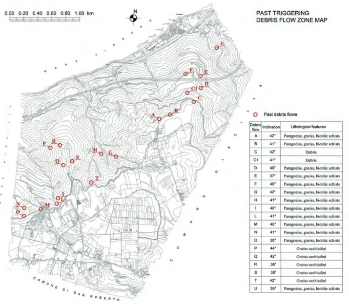
2008b]. Descriptors are parameters or combinations of parameters that are chosen according to: the sca-le of analysis and the related zoning purposes (infor-mation, advisory, statutory and design); the landslide types (potential or existing) and their characteristics. For the studied area, historical data of occurred landslides (Fig. 3) have been analysed in order to obtain the lithological and inclination features of the triggering zones of first-failure landslides invol-ving residual soils of the past debris flows. Slope in-clinations have been evaluated by means of high re-solution digital terrain model (interval contour of 2 m) of the area and the lithological features have be-en obtained by geological map (scale 1:5.000). In fig-ure 3, the letters A, B, C, and C1 refer to the event
in 2001 while the letter F refers to the event in 2005. The analysis of twenty past rapid events (Fig. 4), occurred between 2001 and 2005, has been per-formed in order to define the slope ranges of the events. The obtained results showed that the most part of the events occurred on slope ranges of 38°-40° and 41°-43°, with frequency of the number of the events equal to 40% and 50%, respectively. Moreover, the past events occurred on debris and on alteration soils coming from paragneiss, gneiss and biotitic schists, and gneiss occhiadini.
Fig. 2 – 2001 and 2005 rapid debris flows: triggering zones, propagation and accumulation areas.
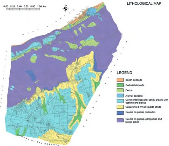
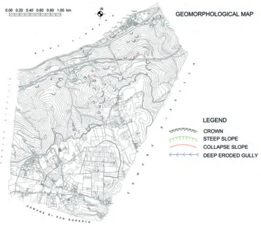
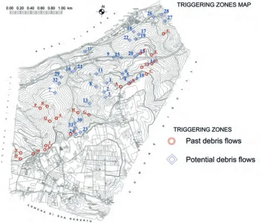
On the base of available information, the source areas of potential landslides have been predicted using an heuristic method based on observed phe-nomena and on lithological (Fig. 5), inclination (Fig. 6) and geomorphological (Fig. 7) setting of the area. In particular, detailed and validated in field thematic maps (maps drawn for the design of the new double three-phase 380 kV powerline) have be-en used to evaluate potbe-ential triggering areas of de-bris flows. For this purpose, the slope inclinations, li-thological features and geomorphological evidences (crowns, deep eroded gullies, steep and collapse slo-pes) have been selected as qualitative susceptibility descriptors. The potential triggering zones of debris flows (Fig. 8) have been obtained overlapping three thematic layers (Figs. 5, 6, 7).
Potential and past debris flow triggering zones of the area are shown in figure 9, where blue squa-res repsqua-resent the predicted potential triggering
zo-Fig. 3 – Map of the past real debris flows occurred in the studied area.
Fig. 3 – Mappa delle aree di innesco di debris flow avvenuti nell’area di studio.
Fig. 4 – Frequency of the number of events versus slope ranges and involved lithology.
Fig. 4 – Frequenza del numero di eventi in funzione degli intervalli di inclinazione e delle litologie coinvolte.
52 MORACI - MANDAGLIO - GIOFFRÈ - PITASI
Fig. 5 – Lithological map of the studied area.
Fig. 5 – Mappa litologica dell’area di studio.
Fig. 6 – Inclination map of the studied area.
Fig. 7 – Geomorphological map of the studied area.
Fig. 7 – Mappa geomorfologica dell’area di studio.
Fig. 8 – Potential debris flow map of the studied area.
54 MORACI - MANDAGLIO - GIOFFRÈ - PITASI
nes while red circles represent the zones where the past debris flows occurred.
The mapping shown in figure 9 represents the result of the first stage in the proposed approach. Calibration of the rheological law
In order to study the propagation phase, it is im-portant to define the rheological model of the debris flow mixture. Definition of rheological model is fun-damental for the numerical analyses to evaluate the debris flow paths (runout), velocities and heights du-ring the propagation phase.
The soil involved in the rapid debris flows oc-curred in the studied area has been sampled in th-ree different zones near the triggering zones of real past events (Events A and F, Fig. 3). Considering that the past events of debris flows occurred on the same soils, due to the limited variability of lithological and geotechnical features of outcropping soils (residual soils), the sampled soil has been assumed representa-tive as trigger soil mass.
The plastic index and liquid limit of the sampled soil were 9.23 % and 33.27%, respectively. The per-centage of different fractions were: Sand = 30 %, Silt = 45%, Clay = 25%. The soil has been classified accor-ding to the Unified Soil Classification System (USCS) as inorganic silt of medium compressibility with sand
(ML). Besides, in order to obtain the mixture rheolo-gical law, viscometer tests have been performed using the finer percentage (fine sandy, silty and clayey frac-tions) of soils. Tests have been carried out on soil-wa-ter mixtures changing the solid concentration by vo-lume Cv, defined as the ratio between the solid
parti-cles volume and the total volume of the specimen. In particular, between 35% and 45%.
The selection of a particular rheological mo-del is difficult, and several momo-dels can provide si-milar results. Several models have been developed from experimental data got with rheometer, from theoretical considerations and from field observa-tions. Basically, there are different models dedica-ted to the behavior of fluidized geomaterials and the most commonly used ones are: the frictional-turbulent “Voellmy” resistance proposed initially for snow avalanches and used for granular cohe-sionless materials with or without the presence of a pore fluid; the visco-plastic Bingham-type resistan-ce relationship applicable for plastic clay-rich ma-terial [MALET et al., 2004; PASTOR et al., 2009].
Ac-cording to RICKENMANN et al. [2006], a clay fraction
(particle size less than 40 µm) greater than 10% is necessary for a flow material to behave like a Bing-ham fluid.
For the studied case, previously [GIOFFRÈ et al.,
2016], a parametric analysis using Voellmy model and Bingham model, was carried out, showing that
Fig. 9 – Triggering zone map of the studied area.
the last one represents better the zoning resulting from the real event of 2001.
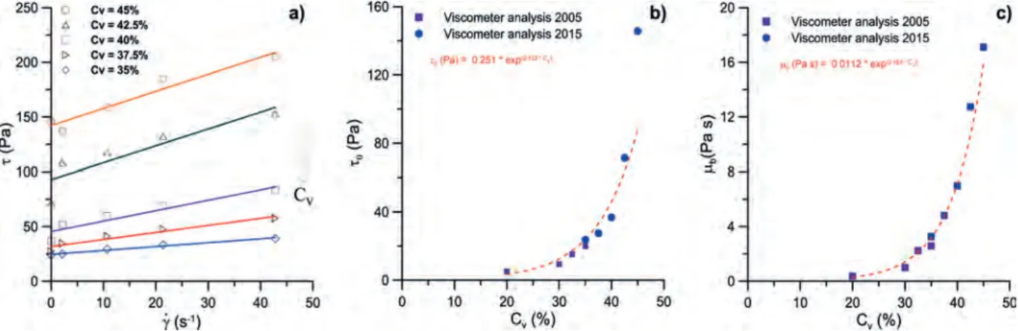
Once the model was selected, viscometer labo-ratory tests have been performed to derive the Bing-ham model parameters (o and b) as a function of
the solid concentration (Cv). The figure 10a shows
that the shear stress linearly increases with increa-sing of the shear rate. Moreover, results show that an increase of Cv leads to an increase of the shear stress.
The viscous Bingham law formulation is: · ·
τ τ= +0 µ γb (1)
where is the shear stress, 0 is yield stress, b is the
Bingham viscosity and ·γ is the shear rate.
The trends of the yield stress and of the visco-sity as a function of the solid concentration by volu-me are shown in figures 10b and 10c.
The results show that both the yield stress (0)
and the viscosity (b) increase exponentially with
in-creasing of the solid concentration by volume, accor-ding to equations, as follows:
·
τ = 0,251 e0 (0,132 C )v (2)
·
µ = 0,0112 eb (0,163 C )v (3) The equations are applicable to flows with Cv less
than 60 % [PIERSON et al., 1987].
Analysis of debris flow propagation phase
The analysis of the rapid debris flow propaga-tion phase is the third stage of the proposed appro-ach. The distinctive features of these landslides are
strictly related to the mechanical and rheological properties of the involved materials, which are re-sponsible together with slope morphometry for long travel distances and the high velocities (order of me-ters/second) that the mass may attain.
The prediction of both run out distances and velocities through mathematical modelling of the propagation stage can notably reduce losses infer-red by these phenomena, as it provides a tool for defining the threatened areas, and for working out the information for the identification and de-sign of appropriate protective measures [MORACI
et al., 2015].
In this study, the numerical model of PASTOR et
al. [2009] has been used to assess the path, the travel distance and the velocity of flowing mass. Numerical simulations of the propagation phase have been per-formed for the past and potential triggering zones shown in figure 9.
In the SPH numerical code, the bed erosion pro-cess is considered implementing the erosion law of HUNGR [1995] using the “growth rate” Es, that
repre-sents the bed-normal depth eroded per unit flow depth and unit displacement, defined as:
=1n(V / )
Es dfin V0 (4)
where Vfin is the final volume of the mobilized
mate-rial, V0 is the initial volume of the debris flow and d is
the travelled distance by debris flow. The numerical code used does not allow us to modify Es along the
path of debris flow [PASTOR et al., 2009; CUOMO et al.,
2014]. Therefore, several numerical simulations ha-ve been carried out using different values of “growth rate”.
In order to validate the results obtained by me-ans of viscometer tests, numerical back-analyses
ha-Fig. 10 – Viscometer results: Shear stress versus shear rate as a function of Cv a); Yield stress 0 versus solid concentration by
volume Cv b); viscosity b versus solid concentration by volume Cv c).
Fig. 10 – Risultati delle analisi con viscosimetro: Sforzo di taglio in funzione del gradiente di velocità al variare di Cv a); Tensione di
snervamento 0 in funzione della concentrazione solida in volume Cv b); viscosità b in funzione della concentrazione solida in volume
56 MORACI - MANDAGLIO - GIOFFRÈ - PITASI
ve been performed on past debris flow occurred in the study area of Favazzina. In particular, the debris flow occurred in May 2001 has been simulated as it is well documented in the literature [BONAVINA et
al., 2005].
For analysing the debris flows, the conditions that occurred on event of May 2001, which affected the Favagreca river for which it was possible a better reconstruction of the geometry and of the volumes of detached mass, were taken into account. In parti-cular, the following parameters were known: initial volume of the detached mass (1130 m3); final
volu-me at the end of the path (Vfin=3V0); pre-event
digi-tal terrain model of the study area.
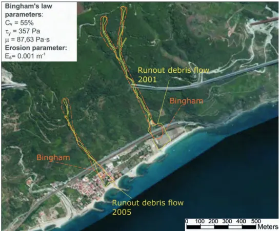
The validation of the numerical model was ba-sed on a trial and error selection of rheological para-meters and of erosion coefficient for the debris flow occurred in May 2001. These values obtained for the debris flow of May 2001 were also used for the debris flow occurred in March 2005 because for this events similar information were not available.
The analyses on the debris flows were carried out assuming the Bingham rheological parameters (yield stress 0 and viscosity b) evaluated by means of
equa-tions (2) and (3) obtained by the viscometer tests for different values of solid concentration by volume Cv
(40-60%). The erosion coefficient Es, assumed equal
to 0.001 m-1, was obtained by the equation (4).
Figu-re 11 shows the Figu-results of numerical simulations, per-formed using Cv =55% and Es = 0.001 m-1,that well
fit the real zoning of the area involved in the debris flows of 2001 and 2005 (yellow lines). It can be noti-ced that the Bingham rheological law well reproduces the runout distances and the geometrical characteri-stics (shape, path, runout zones) of the analysed re-al debris flows. Differences can be noticed at the end of runout zones but they are due to low definition of DEM in these areas, that are extensively urbanized.
Results
Debris flow susceptibility zoning
In order to draw the debris flow susceptibility maps, several numerical simulations of the propa-gation phase of the potential and real triggering zo-nes previously identified (Fig. 9) have been perfor-med and the run-out zones and debris flow paths have been marked.
The Bingham rheological parameters have been varied as a function of the solid concentra-tion by volume Cv and the range of variation of
Cv has been chosen considering the typical values
of debris flows [PIERSON et al., 1987]. The Hungr
erosion coefficient Es has been changed between
Fig. 11 – 2001 and 2005 Favazzina debris flows: comparison between real (yellow lines) and numerical (dotted lines) zoning.
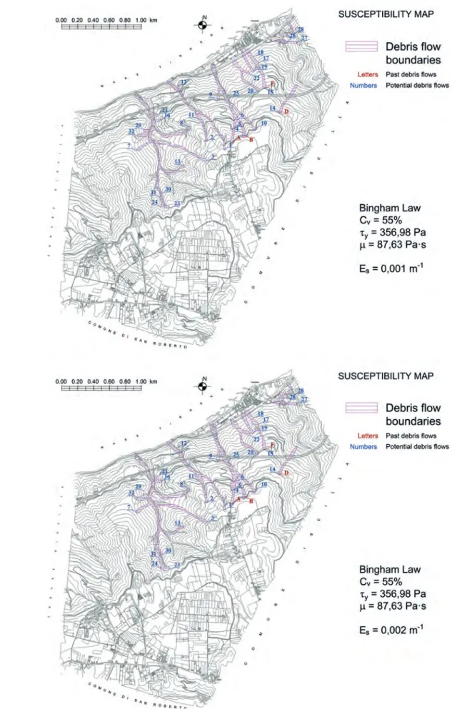
Fig. 12 – Susceptibility maps of the studied area with Cv=55% for Es=0.001m-1 a) and Es=0.002m-1 b).
Fig. 12 – Mappe di suscettibilità dell’area in esame per Cv=55% per Es=0.001m-1 a) e Es=0.002m-1 b). a)
58 MORACI - MANDAGLIO - GIOFFRÈ - PITASI
a)
b)
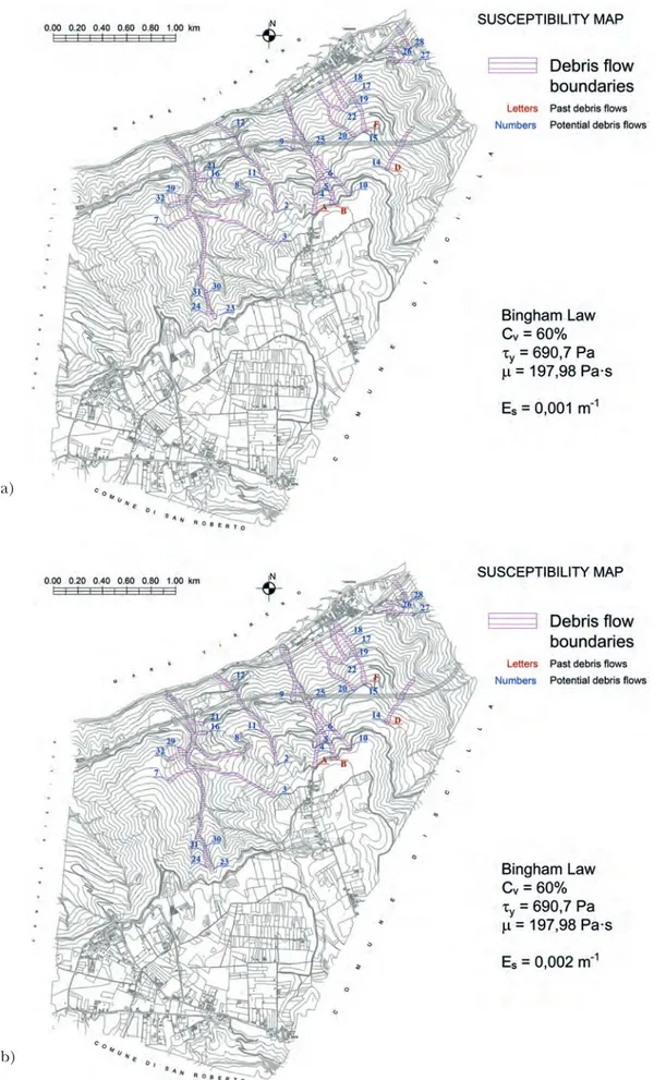
Fig. 13 – Susceptibility maps of the studied area with Cv=60% for Es=0.001m-1 a) and Es=0.002m-1 b).
0.001 m-1 and 0.002 m-1. The initial mobilized
vo-lume depends on the amount of rainfall and its cu-mulative time trend as well as on the morphomet-ry of the specific slope where it triggered. On the base of the geomorphological analyses performed, the initial volume of the detached mass of debris flow 2001 resulted one of the major volumes deta-ched in the studied area. Therefore, this value has been assumed on safe side as initial volume of the potential and real triggering zones in the propa-gation phase for drawing the susceptibility maps.
Ten debris flows susceptibility maps have been obtained for different values of solid concentration by volume Cv (40-45-50-55-60%) and for different Es
(0.001 m-1 - 0.002 m-1). Figures 12-13 show the debris
flows susceptibility maps drawn for the solid concen-tration by volume Cv equal to 55% and 60% and Es
equal to 0,001 m-1 and 0,002 m-1. The maps report
the debris flow path boundaries (magenta zones), obtained by numerical simulations. The zoning has
been performed overlapping for the channels made of more than one incision the obtained numerical results in each simulations.
Comparison between maps with the same Cv
va-lue and different Es shows that the propagation
zo-nes and the run-out areas are wider in the case of Es
equal to 0,002 m-1, as expected.
Moreover, the maps with solid concentration by volume equal to 60% (Fig. 13) show a higher degree of channelling of the debris flows than those with so-lid concentration by volume equal to 55% (Fig. 12); this is due to greater values of velocity obtained for Cv = 55% that produce greater spreading in terms of
displacement of ‘particles’.
In order to choose a safety debris flow susceptibi-lity map for the area, four control sections (I, II, III, IV), in correspondence to the main road SS18, have been chosen (Fig. 14). In these sections, the values of debris flows heights, final volumes and velocities, have been taken by the numerical simulations.
Fig. 14 – Control sections.
60 MORACI - MANDAGLIO - GIOFFRÈ - PITASI
ID Debris flow= debris flow identification; d = travelled distance; Vfin = debris flow final volume; V0 = debris flow initial
vo-lume; hrunout (v = 0) = debris flow height in the deposition area (flow velocity =0); vc.s. = debris flow velocity in the control
section.
ID Debris flow= identificativo del debris flow; d = lunghezza del percorso debris flow; Vfin = volume finale debris flow; V0 = volume iniziale
debris flow; hrunout (v = 0) = altezza del debris flow nella zona di deposizione (velocità del flusso = 0); vc.s. = velocità del debris flow nella
se-zione di controllo.
Section ID
Debris flow
CV 55% 60%
d Vfin/V0 h(v = 0)runout vc.s. Vfin/V0 hrunout = 0)(v vc.s.
(m) (-) (m) (m/s) (-) (m) (m/s) I F 690 1,517 1,22 5,12 1,533 0,79 4,05 17 345 1,348 1,00 5,60 1,349 0,95 2,69 18 290 1,291 0,99 5,13 1,288 1,05 2,42 II 19 385 1,424 0,80 8,50 1,392 0,92 6,40 III 20 630 1,649 1,07 4,46 1,564 1,02 4,30 22 380 1,407 0,60 3,90 1,373 0,79 1,60 IV A 1080 3,157 2,13 7,15 3,031 2,06 6,22 4 1000 2,681 2,22 6,98 2,645 1,67 5,76 5 860 2,182 1,33 7,03 1,749 1,28 5,56 6 800 1,395 1,00 7,09 1,401 0,72 5,40 9 500 1,468 1,12 5,47 1,397 1,11 3,50 10 1016 2,695 2,53 7,08 2,490 1,15 6,09 25 500 1,524 2,30 4,25 1,377 1,32 4,07
Tab. 1 – Results of numerical analysis obtained for Es 0,001m-1, Cv 55% and Cv 60% in the control sections.
Tab. 1 – Risultati dell’analisi numerica ottenuti per Es 0,001m-1, Cv 55% e Cv 60% nelle sezioni di controllo.
The results of numerical analysis obtained for Cv
values equal to 55% and 60% and for Es value equal
to 0,001 m-1 in terms of debris flow height, volume
and velocity values are shown in table I. These va-lues are in accord with those measured for the de-bris flow of 2001. The results obtained for Cv equal
to 55% and Es equal to 0.001 m-1 show greater debris
flow heights and velocities, so the debris flow suscep-tibility map of the studied area shown in figure 12a has been taken up in order to stay on the safe side.
Conclusions
In this paper, an approach to define the debris flow susceptibility of an area, where the lithological and geotechnical features have a limited variability, has been proposed. The used approach provided a good accuracy between predictions against observed data. In particular, the obtained susceptibility zoning maps based on susceptibility descriptors, laboratory tests and numerical analysis are in good agreement with the past events occurred in the area.
Considering that the choice on the most appro-priate zoning method to adopt also depend on
fac-tors, such as the quality and accuracy of the availa-ble data within the area to be zoned, the proposed approach can be considered as a preliminary mixed approach. In fact, the triggering areas of landslides have been predicted using a heuristic method ba-sed on observed phenomena and on geological/ge-omorphological setting of the area whereas the path, the travel distance and velocity of flowing mass have been evaluated by application of a continuum-me-chanics based numerical code.
The results provide a preliminary level of zoning on which more sophisticated studies based on de-terministic methods including physically based mo-del such as SHALSTAB [MONTGOMERY and DIETRICH,
1994] or TRIGRS unsaturated [SAVAGE et al., 2004]
must be developed. Therefore, the proposed appro-ach can be used for information and advisory.
Acknowledgment
All authors have contributed in equal manner to the development of research and to the extension of memory. This research was financially supported by the Italian government within the framework of the
– Suscettibilità alle frane superficiali veloci in terreni di alterazione: un possibile contributo della modellazione del-la propagazione. Rend Online Soc. Geol. It., 21, pp. 534-536.
CASCINI L. (2008) – Applicability of landslide
susceptibil-ity and hazard zoning at different scales. Eng Geol, 102, pp. 164-177.
CROSTA G.B., IMPOSIMATO S., RODDEMAN D.G. (2006)
– Continuum Numerical Modelling of Flow-Like Land-slides. In : Evans S.G. (Ed.,), Landslides from Mas-sive Rock Slope Failure, vol. XLIX of the series NA-TO Science Series, pp. 211-232.
CUOMO S., PASTOR M., CASCINI L., CASTORINO G.C.
(2014) – Interplay of rheology and entrainment in debris avalanches: a numerical study. Canadian Geotechni-cal Journal, 51, n. 11, pp. 1318-1330, doi: 10.1139/ cgj-2013-0387.
FELL R., COROMINAS J., BONNARD C., CASCINI L., LEROI
E., SAVAGE W.Z. (2008a) – Guidelines for landslide
sus-ceptibility, hazard and risk zoning for land use planning. Commentary. Engineering Geology, vol. CII, pp. 99-111 ISSN: 0013-7952.
FELL R., COROMINAS J., BONNARD C., CASCINI L., LEROI
E., SAVAGE W.Z. (2008b) – Guidelines for landslide
sus-ceptibility, hazard and risk zoning for land use planning. Engineering Geology, n. 102, pp. 85-98.
GEOPORTALE NAZIONALE
http://www.pcn.minambien-te.it/GN.
GIOFFRÈ D., MORACI N., BORRELLI L., GULLÀ G. (2016)
– Numerical code calibration for the back analysis of de-bris flow runout in Southern Italy. Landslides and En-gineered Slopes. Experience, Theory and Practice: Proceedings of the 12th International Symposium
on Landslides, n. 2, pp. 991-997.
GULLÀ G., MANDAGLIO M.C., MORACI N. (2006) – Effect
of weathering on the compressibility and shear strength of a natural clay. Canadian Geotechnical Journal, n. 43, pp. 618-625.
GULLÀ G., MANDAGLIO M.C., MORACI N. (2005) –
Influ-ence of degradation cycles on the mechanical characteris-tics of natural clays. Proceedings of the 16th
Interna-tional Conference on Soil Mechanics and Geotech-nical Engineering, Osaka (Japan), 12-16 Septem-ber 2005, pp. 2521-2524.
per #4. Taylor and Francis Group, London, pp. 99-128.
HUNGR O., PICARELLI L., LEROUEIL S. (2014) – The
Var-nes classification of landslides-an update. Landslides, 11, pp. 167-194.
HÜRLIMANN M., RICKENMANN D., MEDINA V., BATEMAN A.
(2008) – Evaluation of approaches to calculate debris-flow parameters for hazard assessment, Eng. Geol., n. 102, pp. 152–163.
IVERSON R.I., GEORGE D.L. (2014) – A depth-averaged
debris-flow model that includes the effects of evolving di-latancy. I. Physical basis. Proc. Royal Society, Series A, 470.
JACOB M., HUNGR 0. (2005) – Debris-flow Hazards and
Related Phenomena. Spinger.
LEE E.M., JONES D.K.C. (2004) – Landslide risk
assess-ment. Thomas Telford Ltd, London.
MALET J.P., REMAÎTRE A., MAQUAIRE O. (2004) –
Run-out modeling and extension of the threatened area associ-ated with muddy debris flows. Géomorphologie: relief, processus, environnement. 3, pp. 195-210.
MANDAGLIO M.C., MORACI N., GIOFFRÈ D., PITASI A.
(2015) – Susceptibility analysis of rapid flowslides in southern Italy. Proceedings of International Symposium on Geohazards and Geomechanics (ISGG2015). War-wick, UK. Earth and Environmental Science 26. doi: 10.1088/1755-1315/26/1/012029.
MANDAGLIO M.C., MORACI N., GIOFFRÈ D., PITASI A.
(2016) – A procedure to evaluate the susceptibility of rapid flowslides in Southern Italy. Landslides and Engineered Slopes. Experience, Theory and Prac-tice: Proceedings of the 12th International
Sympo-sium on Landslides, 3, pp. 1339-1344.
MANDAGLIO M.C., MORACI N., ROSONE M., AIRÒ FARULLA
C. (2016) – Experimental study of a naturally-weathered stiff clay. Canadian Geotechnical Journal, 10.1139/ cgj-2016-0175. 53 n. 6, pp. 946-961.
MORACI N., PISANO M., MANDAGLIO M.C., GIOFFRÈ D.,
PASTOR M., LEONARDI G., COLA S. (2015) – Analyses
and design procedure of a new physical model for debris flows: results of numerical simulations by means of labora-tory tests. IJEGE Italian Journal of Engineering Geo-logy and Environment. doi: 10.4408/IJEGE.2015-02.O-03.
62 MORACI - MANDAGLIO - GIOFFRÈ - PITASI
PASTOR M., HADDAD B., SORBINO G., CUOMO S., DREM -PETIC V. (2009) – A depth integrated coupled SPH
mod-el for flow-like landslides and rmod-elated phenomena. In-ternational Journal for Numerical and Analytical Methods in Geomechanics, 33, n. 2, pp. 143-172. PASTOR M., BLANC T., MANZANAL D., DREMPETIC V., PAS
-TOR M.J., SÁNCHEZ M., CROSTA G., IMPOSIMATO S., ROD -DEMAN D., FOESTER E., KOBAYASHI H., DELATTRE M.,
ISSLER D. (2012) – Deliverable D1.7 Landslide runout:
Review of analytical/empirical models for subaerial slides, submarine slides and snow avalanche. Numerical mod-elling. Software tools, material models, validation and benchmarking for selected case studies. Safeland Pro-ject. Living with landslide risk in Europe: Assess-ment, effects of global change, and risk manage-ment strategies.
PEZZINO A., PANNUCCI S., PUGLISI G., ATZORI P., IOPPOLO
S., LO GIUDICE A. (1990) – Geometry and metamorphic
environment of the contact between the Aspromonte-Pelo-ritani Unit (Upper Unit) and Madonna dei Polsi Unit (Lower Unit) in the central Aspromonte area (Calabria). Bollettino della Società Geologica Italiana, 109, pp. 455-469.
PIERSON T.C., COSTA J.E. (1987) A rheologic
classifica-tion of subareal sediment flows. Reviews in Engineer-ing Geology. VII Debris flow / Avalanches: process, recognition and mitigation, J.E. Costa and Wiec-zoreck (Eds.), Geolocical Society of America, Boul-der, Colorado, 7, pp. 1-12.
PIRULLI M., PASTOR M. (2012) – Numerical study of the
entrainment of bed material into rapid landslides. Géo-technique, n. 62, pp. 959–972.
RICKENMANN D., LAIGLE D. MCARDELL B. W., HÜBL J.
(2006) – Comparison of 2D debris flow simulation models with field events. Computat. Geosci., 10, pp. 241-264.
SAVAGE W.Z., GOD J.W., BAUM R.L. (2004) – Modelling
time-dependent areal slope instability. In: Lacerda W.A., Ehrlich M., Fontoura S.A.B., Sayao A.S.F. (Eds.) Landslides – Evaluation & Stabilization, Proceed-ings of the 9th International Symposium on
Land-slides, 28 June – 2 July 2004, Rio de Janeiro, A.A. Balkema Publishers, vol. I, pp. 23-38.
Zonazione della suscettibilità da frana di
colata detritica: un approccio applicato a
un’area studio
Sommario
L’articolo presenta un approccio per la zonazione della suscettibilità da frana di colata detritica applicato a un’area della provincia di Reggio Calabria (Italia), periodicamente soggetta a frane di colata rapida innescate da piogge. In particolare, utilizzando un metodo euristico basato sui fenomeni osservati e sulle caratteristiche geologiche/geomorfologiche dell'area in esame, sono state individuate le aree di potenziale distacco di colate detritiche. Successivamente, è stata analizzata con un metodo avanzato (modello numerico) basato sulla caratterizzazione geotecnica e reologica delle coltri di alterazione coinvolte nei fenomeni franosi, la fase di propagazione delle colate detritiche. In tal modo è stato possibile valutare, per ogni colata detritica potenziale o reale, il percorso e le caratteristiche cinematiche (altezza e velocità di propagazione) in corrispondenza di differenti sezioni di controllo poste in prossimità di elementi esposti.
I risultati ottenuti rappresentano un livello preliminare di zonazione della suscettibilità da frana dell’area in base al quale sviluppare studi più sofisticati volti alla mitigazione del rischio.