A study with state space models.
Paolo ChiricoDIGSPES Alessandria University of Eastern Piedmont, Italty
Abstract The paper presents a study of seasonality in Italian daily electricity prices. In particular, it compares the ARIMA approach with the structural state space approach in the case of seasonal data. Unlike ARIMA modeling, the structural approach has enabled us to detect, in the prices under consideration, the presence of stochastic daily effects whose intensity is slowly decreasing over time. This dynamic of seasonality is the consequence of a more balanced consumption of electricity over the week. Some causes of this behavior will be discussed in the final considerations. Moreover, it will be proved that state space modeling allows the type of seasonality, stochastic or deterministic, to be tested more efficiently than when unit root tests are used.
Key words: Electricity prices, seasonal unit roots, HEGY test, structural space state models
1 Introduction
In the past twenty years, competitive wholesale markets of electricity have started in the OECD countries in the international context of the deregulation of energy markets. At the same time, an increasing number of studies on electricity prices have been published. Most of these studies have sought to identify good prediction models, and, for this reason, ARIMA modeling has been the most common methodology. Nevertheless, electricity prices present periodic patterns, seasonality in time series terminology, for which ARIMA modeling does not always seem the best approach.
The treatment of seasonality in the ARIMA framework is conceptually similar to the treatment of trends: like these, seasonality entails the non-stationarity of the process, and its non-stationary effect has to be removed before modeling the process. More specifically, if the seasonal effects are constant at corresponding times (e.g. every Sunday, every Monday,...,), the seasonality can be represented by a periodic linear function s(t) (deterministic seasonality). In this case, the correct treatment consists in subtracting the seasonality, and then in modeling the non-seasonal prices using an ARIMA model:
φ(B)∆[pt− s(t)] =θ(B)εt1 (1)
On the other hand, if the seasonal effects are characterized by stochastic variability (stochas-tic seasonality), the correct treatment consists in applying the seasonal difference to the prices This is a post-peer-review, pre-copyedit version of an article published in Topics in Theoretical and Applied Statistics by Springer
1Formally, model 1 is called the Reg-Arima model by some authors, ARMAX by others.
∆spt= pt− pt−s, and then modeling the differences using an ARIMA model:
φ(B)∆∆spt =θ(B)εt (2)
The two treatments are not interchangeable. In fact, in the case of deterministic seasonality, the seasonal difference is not efficient because it introduces seasonal unit roots into the moving average partθ(B) of the ARIMA model; in the case of stochastic seasonality, the first treatment does not assure stationarity in the second moment of the data [6]. Hence, the correct application of ARIMA models to seasonal data requires first the identification of the type, stochastic or deterministic, of the seasonality present in the prices.
In many cases, statistical tests indicate the presence of deterministic seasonality, at least in the short run. For this reason, as well as for easiness reasons, many scholars ([1, 12, 9]) have opted for representing seasonality by means of periodic functions. This approach makes it possible to measure the seasonal effects, but it is based on the strong assumption that seasonal effects remain constant over time. On the other hand, the seasonal difference approach does not satisfy the need to under-stand and model the real dynamic of seasonality in electricity prices. Therefore, other scholars [10] turned to periodic ARIMA models, but this modeling requires numerous parameters when season-ality presents numerous periods (e.g. daily pattern). On the basis of these considerations, Structural State Space Models could be a solution for representing seasonality in a flexible way, but using few parameters. The paper illustrates some structural space state models that yielded interesting find-ings about seasonality in Italian daily electricity prices. More specifically, the paper is organized as follows. The next section illustrates some items about deterministic and stochastic seasonality, and the most common test for checking seasonality is presented. In Section 3, an analysis of the Italian daily electricity prices is discussed, comparing the ARIMA approach with the structural (space state) approach. Final considerations are made in the last Section.
2 Deterministic and stochastic seasonality
Seasonality can be viewed as a periodic component stof a seasonal process ytthat makes the process
non-stationary:
yt= ynst + st (3)
The remaining part yns
t = yt− stis the non-seasonal process and is generally assumed stochastic, but
st can be either deterministic or stochastic.
Deterministic seasonality can be represented by periodic functions of time (having s periods) like the following ones:
st= s
∑
j=1 γjdj,twith s∑
j=1 γj= 0 (4) or st= [s/2]∑
j=1 Ajcos(ωjt −φj) (5)In equation 4, the parameterγj represents the seasonal effect in the j-th period (dj,t is a dummy
variable indicating the period). In equation 5, seasonality is viewed as the sum of[s/2]2harmonic functions each of them having angular frequencyωj= j2π/s; j = 1, 2,..., [s/2]. Deterministic
sea-sonality satisfies the following relation:
2
S(B)st= 0 (6)
where S(B) = 1 + B + B2+ ... + Bs−1 is the seasonal summation operator based on the backward
operator B3. In the case of stochastic seasonality, the relation 6 becomes:
S(B)st= wt (7)
where wtis a zero-mean stochastic process (stationary or integrated). Now seasonality can be viewed
as the sum of of[s/2] stochastic harmonic paths hj,t:
γj(B)hj,t= wj,t (8)
where
γj(B) = (1 − eiωjB)(1 − e−iωjB) if 0 <ωj<π (9)
γj(B) = (1 + B) ifωj=π (10)
and wj,tis a zero-mean stochastic process (stationary or integrated).
Since each seasonal operatorγj(B) is a polynomial with unit roots, each stochastic harmonic path
implies the presence of one or two (complex and conjugate) unit roots in the process (more exactly, in the autoregressive representation of the process) and vice-versa. Finally, since:
∆s=∆S(B) =∆ [s/2]
∏
j=1γj(B) (11)
the application of the filter∆s to a seasonal process yt makes the process stationary, removing a
stochastic trend (eventually present in the non-seasonal data) and[s/2] stochastic harmonic paths present in seasonality.
2.1 HEGY test
A very common methodology used to test for non-stationarity due to seasonality is the procedure developed by Hylleberg, Engle, Granger, and Yoo [8], and known as the HEGY test. This test was originally devised for quarterly seasonality, but it has also been extended for weekly seasonality in daily data by Rubia [13].
Under the null hypothesis, the HEGY test assumes that the relevant variable is seasonally inte-grated. This means, in the case of daily electricity prices (pt), that the weekly difference∆7pt is
assumed to be a stationary process. Since: ∆7= (1 − B) 3
∏
j=1 (1 − eiωjB)(1 − e−iωjB) (12) (ωj= 2π/7, 4π/7, 6π/7), the null hypothesis of the HEGY test entails the presence in the processof seven unit roots: one at zero frequency (corresponding to a stochastic trend) and three pairs of complex unit roots corresponding to three stochastic harmonic paths with frequencies 2π/7, 4π/7, 6π/7.
The test consists in checking the presence in the process of the unit roots; in this sense it can be
3S(B)s
viewed as an extension of the Dickey-Fuller tests [2]. Like these tests, the HEGY test is based on an auxiliary regression: ∆7pt=α+ 7
∑
s=2 γsds,t+ 7∑
r=1 αrzr,t−1+ p∑
j=1 φj∆7pt− j+εt4 (13)where ds,tis a zero/one dummy variable corresponding to the s-th day of the week, and each regressor zr,tis obtained by filtering the process ptso that:
• it will be orthogonal to the other regressors;
• it will include only one root of the seven roots included in pt.
For example, z1,t includes only the unit root having zero frequency (stochastic trend), but not the
seasonal roots; z2,t and z3,t include only the seasonal roots having frequency 2π/7, and so on (see
[13] for more details).
The number p of lags of the dependent variable in the auxiliary regression (augmentation) has to be chosen to avoid serial correlation in the error termεt.
If∆7pt is a stationary process, all roots have been removed, and the coefficientsαs are not
sig-nificant. As in the augmented unit root test of Dickey and Fuller (ADF), the null hypothesisα1= 0 is accepted against the alternative hypothesisα1< 0 on the basis of a non-standard t-statistic. In regard to the seasonal roots, the test should be performed on each couple of roots having the same frequency. Indeed, only the hypothesisα2 j=α2 j+1= 0 (k = 1, 2, 3) means the absence in∆7pt(i.e.
the presence in pt) of an harmonic path with frequency 2πj/7. This assumption can be tested by a
joint F-test; the distribution of each statistic Fjis not standard, but the critical values are reported in
[11]. In conclusion: if some hypothesisα2 j=α2 j+1= 0 is not rejected, the seasonality should be
stochastic; if all the hypothesesα2 j=α2 j+1= 0 are rejected and some coefficientγsis significant,
the seasonality should be deterministic.
3 Analysis of the Italian daily electricity prices
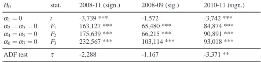
The HEGY test was performed on the 2008-2011 Italian daily PUN5 (more specifically the log-PUN). As reported in Table 1, none of the null hypotheses (H0) was significant at 1% level. Nev-ertheless, the absence of a stochastic trend was not confirmed by the ADF test on the same data. This might mean that the prices process is nearly a stochastic trend, but also that the process is not homogeneous over the whole period. Indeed, after performing the HEGY test on the sub-periods 2008-09 and 2010-11, it can be noted that the statistic t concerning the presence of a stochastic trend gives different signals: the 2008-09 daily prices seem to include a stochastic trend, whereas the 2010-11 daily prices do not. Such deductions were confirmed by performing the ADF test on the data (Table 1). The absence of mean-reversion in the first period is a particular case and should be related to the high variation of the oil prices in the same period. On the other hand, seasonality remains non stochastic in both periods (absence of seasonal roots). According to these findings, the 2008-09 daily log-PUN was represented by a Reg-ARIMA model, but the 2010-11 Log-PUN by a Reg-ARMA model: more specifically, a Reg-IMA(1,2) for the first period and a Reg-AR(7) for the second one. In both cases the regression was the following:
4This is a standard version of the HEGY test for daily data, but it can be extended to include trends. Nevertheless, in
this case, there is no reason for doing so.
5The PUN is the National Single Price in the Italian electricity market (IPEX). The PUN series are downloadable
Table 1 HEGY and ADF tests
H0 stat. 2008-11 (sign.) 2008-09 (sig.) 2010-11 (sign.)
α1= 0 t -3,739 *** -1,572 -3,742 ***
α2=α3= 0 F1 163,127 *** 65,480 *** 84,874 ***
α4=α5= 0 F2 175,639 *** 66,215 *** 90,891 ***
α6=α7= 0 F3 232,567 *** 103,114 *** 93,018 ***
ADF test τ -2,288 -1,167 -3,371 **
pt=γMondMon,t+ ... +γSatdSat,t+ pnst (14)
The models parameters and their significance are reported in Table 2.
Since the analyzed data are log-prices, each daily coefficient (lower part of the table) indicates the average per-cent difference between the corresponding daily price and the Sunday price, which is obviously the lowest price. Indeed, the consumption of electricity is generally lowest on Sundays. To be noted is that the daily effects are lower in the second period. This result may mean that there was a structural break in the seasonality as a consequence of a structural break in the daily demands or in the daily supplies of electricity. On the other hand, seasonality may have had fluctuations of slowly decreasing intensity in the period 2008-2011 as a consequence of slow changes in the daily demands and/or daily supplies of electricity.
In order to gain better understanding of the dynamics of seasonality in the electricity prices, we analyzed the prices by means of state space models.
Table 2 Models parameters
model 2008-09 model 2010-11
param. value/sign. value/sign.
const -0,001 4,136 *** AR1 - 0,351 *** AR2 - 0,116 *** AR3 - 0,084 ** AR4 - 0,134 *** AR5 - 0,088 ** AR6 - 0,038 AR7 - 0,067 * MA1 -0,498 *** -MA2 -0,237 *** -Mon 0,148 *** 0,076 *** Tue 0,173 *** 0,093 *** Wed 0,190 *** 0,091 *** Thu 0,169 *** 0,097 *** Fri 0,151 *** 0,080 *** Sat 0,103 *** 0,072 ***
3.1 State Space analysis of electricity prices
pt = mt+ st+εt (15)
mt+1 = mt+ bt+ε1,t (16)
bt+1 = bt+ε2,t (17)
st+1 = −st− st−1− ... − st−5+ε3,t (18)
where mtis the non-seasonal level of the log-PUN pt; bt is the slope and st is the seasonality (daily
effect). The disturbance factorsεt,ε1,t,ε2,t andε3,t are white noises with variancesσ2,σ12,σ22and σ2
3.
This model, also known as the local linear trend model with seasonal effect [3], is a common starting state space model for seasonal data. Equation 18 is a particular case of assumption 7 (wtis assumed
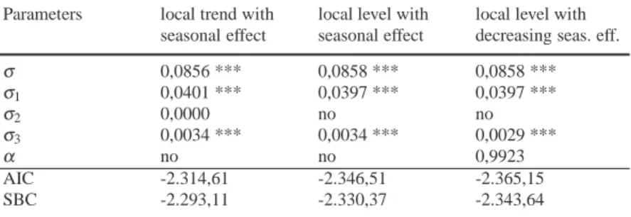
to be a white noise) and entails stochastic seasonality. This assumption permits seasonality to change in the period 2008-2010 according to the findings in Table 1. The estimation results of this model are reported in the second column of Table 3. To be noted is that the estimate of the standard deviation ofε2is zero, which means the slope of the trend bt can be assumed to be non stochastic; moreover,
the estimate of bt converges to zero. For these reasons, a seasonal model without slope (without bt
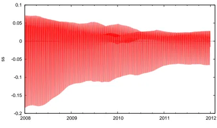
in equation 16 and without equation 17), also known as the local level with seasonal effect, shows better indices of fit (third column). The consideration of the diagram of the smoothed seasonality
Table 3 Three state space models for the log-prices
Parameters local trend with local level with local level with seasonal effect seasonal effect decreasing seas. eff.
σ 0,0856 *** 0,0858 *** 0,0858 *** σ1 0,0401 *** 0,0397 *** 0,0397 *** σ2 0,0000 no no σ3 0,0034 *** 0,0034 *** 0,0029 *** α no no 0,9923 AIC -2.314,61 -2.346,51 -2.365,15 SBC -2.293,11 -2.330,37 -2.343,64
(Figure 1) shows that the daily effects tend to decrease in the period 2008-2011 (in this case, the daily effects should be viewed as the percentage deviations, positive on working days and negative at weekends, from the trend of prices). According to this evidence, the standard local level model was modified by the following seasonal state equation:
st+1= −α(st+ st−1+ ... + st−5) +ε3,t (19)
where 0<α < 1 so that the daily effects can tend to decrease. On performing the new model on the 2008-2011 log-PUN, the value of alpha resulted equal to 0,9923 (Table 3, fourth column); the standard deviation of the disturbance on seasonality was equal to 0,0029 (less than 0, 3%). The values of the Akaike (AIC) and Schwarz (SBC) indices are less than in previous models, denoting an improvement in fit. These findings prove that the daily effects were very slowly decreasing in the period 2008-2011; indeed, so slowly decreasing and so little varying that they could be viewed as constant in a short period. For this reason, the HEGY test, which is not a particularly powerful test, detected deterministic seasonality (Table 1).
-0.2 -0.15 -0.1 -0.05 0 0.05 0.1 2008 2009 2010 2011 2012 ss
Fig. 1 Seasonality in the period 2008-2011
4 Final considerations
The analysis described in the previous sections has shown that the daily effects (i.e. seasonality) on daily wholesale electricity prices exhibited slowly decreasing intensity in the period 2008-11 in Italy. We reiterate that the daily effects can be viewed as deviations from the trend of the prices due to the days of the week. A reduction of the daily effects means a reduction of the differences among the daily prices. Some causes regarding the demand and the supply of electricity can be highlighted. In regard to the demand, a more balanced consumption of electricity over the week has been noted in recent years. One reason is certainly that more and more families have subscribed contracts of domestic electricity provision which make electricity consumption cheaper in the evenings and at weekends. Moreover, the difficulties of the Italian economy in recent years have caused a reduction in electricity consumption on working days.
In regard to the supply, the entry into the market of several small electricity producers has made the supply of electricity more flexible.
Regarding the methodology, Structural State Space Models seem to be a more powerful tool than the HEGY test for detecting the type of seasonality. From the state sequence of the seasonal com-ponents, it is possible to gain a first view on the kind of seasonality affecting the data. Moreover, the significance test on the standard deviation of the disturbance in the seasonal component makes it possible to check whether or not seasonality is stochastic. More specifically, if the standard devia-tion is not significant, the seasonality should be assumed to be deterministic; otherwise it should be assumed stochastic. Although these models are not usually employed for electricity prices, they have interesting features for the analysis and prediction of electricity prices. As known, State Space mod-eling can include ARIMA modmod-eling, but it allows easier modmod-eling of periodic components compared with the latter. Moreover, Structural State Space models can represent electricity prices according to an economic or behavioral theory.
This study has not dealt with volatility clustering, a well-known feature/problem of electricity prices. As known, the GARCH models (in all versions) are typically used to model volatility clus-tering. Although such modeling is generally associated with ARIMA modeling, conditional het-eroscedasticity can be considered in structural framework as well ([7]).
References
1. Bhanot, K.: Behavior of power prices: implications for the valuation and hedging of financial contracts, Journal of Risk, Vol. 2, pp. 43-62. (2000)
2. Dickey, D.A., Fuller, W.A.: Distribution of the estimators for autoregressive time series with a unit root. Journal of American Statistical association, 74, 427–431 (1979)
3. Durbin, J., Koopman, S. J.: Time series analysis by state space methods, Oxford University press. (2001). 4. Escribano et al.: Modelling electricity prices: international evidence, Economic Series 08, Working Paper 02-27,
Universidad Carlos III de Madrid, June. (2002)
5. Gianfreda, A., Grossi, L.: Forecasting Italian electricity zonal prices with exogenous variables, Energy Eco-nomics (available on line: http://dx.doi.org/10.1016/j.eneco.2012.06.024). (2012)
6. Hamilton, J.D.: Time series Analysis, Princeton University Press. (1994)
7. Harvey, A., Ruiz, E., Sentana, E.: Unobserved component time series models with ARCH disturbances. Journal of Econometrics 52, 129-157 (1992).
8. Hylleberg, S., Engle, R.F., Granger, C.W.J., Yoo, B.S.: Seasonal Integration and Cointegration. Journal of Econo-metrics, 44, 215–238 (1990)
9. Knittel CR, Roberts MR.: An empirical examination of restructured electricity prices, Energy Economics 27: 791-817. (2005)
10. Koopman, S. J., Ooms, M., Carnero, M. A.: Periodic seasonal reg-ARFIMA-GARCH models for daily electricity spot prices, Journal of the American Statistical Association, 102(477), 16-27(12). (2007)
11. Leon, A., Rubia, A.: Testing for weekly seasonal unit roots in the Spanish power pool. In: Bunn, D.W. (ed.) Modelling prices in Competitive electricity markets, pp. 131-145. Wiley (2004)
12. Lucia, J., Schwartz, E.: Electricity prices and power derivatives: Evidence from the Nordic Power Exchange, Review of Derivatives Research, 5(1), 5-50, January. (2002)
13. Rubia, A.: Testing for weekly seasonal unit roots in daily electricity demand: evidence from deregulated markets. Istituto Valenciano de investigaciones Economicas, WP-2001-21 (2001)