Velocity structure and seismic anisotropy in the crust and upper mantle from Receiver Function analysis: three case studies in Italy

Universit`a degli Studi di Bologna Dottorato di Ricerca in Geofisica

ALMA MATER STUDIORUM UNIVERSIT `A DEGLI STUDI DI BOLOGNA Facolt`a di Scienze Matematiche Fisiche e Naturali

Dottorato di Ricerca Geofisica XXII Ciclo Settore Scientifico-Disciplinare GEO/10

Velocity structure and

seismic anisotropy in the

crust and upper mantle

from Receiver Function

analysis: three case studies

in Italy.

PhD Thesis of:

Tutor:

Dott. Irene Bianchi

Dott. F. P. Lucente

Coordinator:

Prof. M. Dragoni

CONTENTS

1 Introduction 1

2 Deep Structure of the Colli Albani volcanic district (central

Italy) from Receiver Functions analysis. 5

2.1 Introduction . . . 5

2.2 Crustal structure . . . 7

2.3 Data & Method . . . 8

2.3.1 Dipping layer vs anisotropy with a dipping simmetry axis 9 2.4 Inversion Method . . . 9

2.4.1 Parameter space . . . 11

2.4.2 Sensitivity to 3D parameters . . . 13

2.4.3 Errors on layer thickness . . . 17

2.5 Results . . . 17

2.6 Discussion . . . 28

2.7 Conclusions . . . 32

3 Mapping seismic anisotropy using harmonic decomposition of Receiver Functions: an application to Northern Apennines, Italy. 33 3.1 Introduction . . . 34

3.2 Data & Method . . . 36

3.2.1 CCP and Migration . . . 38 3.2.2 Harmonic analysis . . . 39 3.2.3 Symmetry directions . . . 40 3.2.4 Modeling . . . 42 3.3 Results . . . 42 3.3.1 Harmonic analysis . . . 42 3.3.2 Symmetry direction . . . 49 3.3.3 Modeling . . . 51 3.4 Discussion . . . 52 3.5 Conclusion . . . 56 3.6 Supporting material . . . 57 3

3.6.1 Migration . . . 57

3.6.2 Decomposition of the seismic signal . . . 57

4 Custal thickness variations and seismic anisotropy in Southern Apennines (Itlay) from receiver functions. 61 4.1 Introduction . . . 61

4.2 Data and method . . . 62

4.3 Forward modeling . . . 64

4.4 Results . . . 65

4.5 Discussions . . . 70

4.6 Conclusions . . . 74

5 The 2009 L’Aquila (central Italy) earthquake rupture controlled by a high Vs barrier: a Receiver Function application 79 5.1 Introduction . . . 79

5.2 Data & Method . . . 80

5.3 Results . . . 84

5.3.1 AQU . . . 84

5.3.2 FAGN . . . 88

5.4 Discussions . . . 91

5.4.1 Regional structure of the crust . . . 92

5.4.2 Seismogenetic layer . . . 92

5.5 Conclusions . . . 95

CHAPTER

ONE

Introduction

The most heterogeneous layer of the Earth is the outer one, the crust. Here, chemical composition, rocks texture and physical properties can be highly vari-able in all directions, making the one-dimensional approximations, as function of depth only, extremely rough. The high grade of heterogeneity of the Earth’s crust makes the determination of its principal characteristic (composition, struc-ture, geometry) a difficult task to achieve. This is especially true for the deeper part of the crust, which is not directly accessible, and whose characteristics should be investigated through indirect information. Seismology is possibly the main source of information on the deep Earth, hence on the Earth’s crust. In the last years, the developing of new techniques of analysis and the grow-ing amount of seismological data and studies allowed to gain a better knowl-edge of the Earth’s interior. These studies revealed that the Earth is highly three-dimensional and mainly anisotropic, and these complexities heighten in the crust. In this PhD Thesis we aim to study the crustal structure in various tectonic environments in Italy by means a seismological approach. The Italian territory is shaped by the geodynamic evolution of the Apennines-Tyrrhenian subduction system. Evidence of lithosphere subduction during the Neogene formation of the Apenninic belt comes from geological, petrologic, and seismo-logical studies (Faccenna et al., 2001, and references therein). The present-day geologic setting of the Italian peninsula is complex due to the interaction of different geodynamic processes still acting. Italy is located between the African and the European plates, which are presently converging approximately in a NS direction at a rate of less than 1 cm/year (Argus et al., 1989; Dewey et al., 1989). The present configuration of the Apennines consists of two major arcs, the northern Apennines and the Calabrian arc, separated, in central-southern Apennines, by a NS trending fault zone that, according to some authors is related to deep lithospheric discontinuity (Patacca & Scandone, 1989; Amato et al., 1993; Lucente et al., 1999). It is widely accepted that the southern Tyrrhenian Sea formed as a back-arc basin related to the subduction of the Ionian lithosphere beneath the Calabrian arc (Malinverno & Ryan, 1986). The

northern Apenninic arc developed with a series of thrusting episodes over the Adriatic continental plate, which flexed below the foredeep for as much as 8 km since Pliocene (Royden et al., 1987). The presence of subcrustal seismic-ity down to 90 km depth (Selvaggi & Amato, 1992) suggests that the arc has developed due to westward subduction of the Adriatic plate. In the northern Apennines, from Upper Miocene to Quaternary the coexistence of extension in the internal domain toward the Tyrrhenian, and compression along the external part of the arc, toward the Adriatic, is observed (Patacca & Scandone, 1989; Frepoli & Amato, 1997). Quaternary caldera complexes grown in the back-arc region of the northern Apennines and central Italy. The Central and South-ern Apennines developed in a transition area linking the NorthSouth-ern Apennines and the Calabrian subduction arcs; together they made up the whole Apennine fold-and-thrust belt. From north to south, the Apennines are made of sedimen-tary rocks mainly derived from the Mesozoic deposits of the southern passive margin of the Tethys Ocean, characterized by extensive outcrops of Apenninic Platform carbonate rocks and related transitional facies of pelagic Basin to the north and east. Being locus of very active tectonic processes, the internal structure of the crust in the Italian region is extremely complex. We focus our study on the determination of the main geometric and structural characteristic of some of these crustal complexities. To do it we apply a well know geophysical technique developed to identify the main impedance contrasts in the structure under the seismic station, which uses the analysis of the Receiver Functions (Langston, 1979). These are time series obtained by the teleseismic recordings under a three component seismic station, and recovered thanks to two simple assumptions: that energy from a P-wave which crosses a seismic discontinuity is partially converted into a S-wave, and that for teleseismic P-waves, source and path effects are recorded on the vertical component. Through the deconvo-lution of the horizontal components from the vertical one of the seismic record, we obtain two times series, Radial and Transverse, which contain the P-to-S phases converted at the interfaces under the receiver. In a receiver function the local structure response is separated by all other factors which interact to compose a seismogram, the information is then translated into a simple model of local velocity structure. We analyzed and modeled the computed receiver functions to generate S-velocity models of the crust and upper mantle in vari-ous study regions, in Italy. We often find and model not only one-dimensional structures below the stations, but more often our results evidence the presence of crustal complexities, such as dipping interfaces and anisotropic layers. In particular, the determination of the anisotropic properties of rocks both in the crust and in the mantle can be highly informative on their tectonic history and on the stress regime acting. The tectonic processes that we observe in nature impose stresses and shear on the Earth outermost layers, these forces deform the crust and mantle, modifying their internal structure, and reorganizing the texture of rocks. This can cause differential propagation of the seismic waves inside the Earth’s interior, i.e. the seismic anisotropy. The mechanisms that are used to explain anisotropy in the crust and the mantle are usually classified in two main groups: shape-preferred orientation (SPO) and lattice-preferred orientation (LPO) of Earth materials (e.g. Fouch & Rondenay, 2006). In the

3

Earth’s crust the development of anisotropy is generally ascribed to SPO related to structural features as faults, regularly oriented cracks or layering, or due to elongated or flat minerals alignment, that provide a preferential fast and slow direction of seismic wave propagation. In the upper mantle, seismic anisotropy is usually caused by LPO of crystallographic axes of olivine, which is the main constituent of the Earth’s mantle, and which fast symmetry axis aligns roughly parallel to the direction of maximum extension or is controlled by the flow di-rection. Therefore, seismic anisotropy can be highly informative on the past (inherited) and present tectonics. In this PhD Thesis we retrieve the crustal model in three different regions in Italy: 1) the Colli Albani volcanic district. This is a geographically limited area SE of Rome, which has been interested by recent (Quaternary) magmatic activity. The Colli Albani Volcano is one of the several volcanoes and caldera complexes developed starting from Pliocene along the Tyrrhenian coast and forming the Roman Magmatic Province. 2) The Northern Apennines. The northern Apenninic arc is the surface expression of the subduction process of the northernmost segment of the Adria lithosphere beneath the Tyrrhenian basin. The grown of the mountain chain is related to the emergence of the accretionary prism that developed within the subduction zone. At present the subduction process here has slowed or perhaps terminated due to the exhaustion of the oceanic or thinned continental crust available for subduction, even if the signature of subduction is preserved. 3) The Southern Apennines. Southern Apennines is characterized by extensive outcropping of carbonate platform rock. It has been theatre of large and destructive earth-quakes in the past, and is locus of the main hydrocarbon reservoir on land in Italy. Despite of the extensive oil exploration, the deeper portion of the crust here is largely unknown.

As additional case of study, since the exceptional nature of the event, we explore the crustal structure in the epicentral area of the earthquake, which struck L’Aquila in the 2009.

In the following chapters crustal structure and properties of the above dif-ferent regions will be discussed in detail.

CHAPTER

TWO

Deep Structure of the Colli Albani volcanic district

(central Italy) from Receiver Functions analysis.

The Colli Albani is a Quaternary quiescent volcano, located a few kilometers southeast of Rome (Italy). During the past decade, seismic swarms, ground deformation and gas emissions occurred in the southwestern part of the vol-cano, where the last phreatomagmatic eruptions (27 ky) developed, building up several coalescent craters. In the frame of a DPC-INGV project aimed at the definition and mitigation of volcanic hazard, a temporary array of seismic stations has been deployed on the volcano and surrounding areas. We present results obtained using Receiver Functions (RF) analysis for 8 stations, located upon and around the volcanic edifice, and revealing how the built of the volcanic edifice influenced the pre-volcanic structures. The stations show some common features: the Moho is almost flat and located at 23 kilometers, in agreement with the thinning of the Thyrrenian crust. Also the presence of a shallow lime-stone layer is a stable feature under every station, with a variable thickness between 4 and 5 km. However, some features change from station to station, indicating a local complexity of the crustal structure: a shallow discontinuity dividing the Plio-Pleistocenic sediments by the Meso-Cenozoic limestones, and a localized anisotropic layer, in the central part of the old strucure, which points of the deformation of the limestones. Other two strongly anisotropic layers are detected under the stations in lower crust and upper mantle, with symmetry axis directions related to the evolution of the volcano complex.

2.1

Introduction

The Colli Albani volcanic district, is one of the several Quaternary caldera complexes developed in the back-arc region of the northern Apennines (Fac-cenna et al., 1997, 2001) (see Figure 2.1). It is characterized by hyper-potassic magma originated during the wide extensional processes by partial melting of a K-metasomatised mantle source (Sartori, 1990; Conticelli & Peccerillo, 1992; Faccenna et al., 2001).

12˚30' 12˚30' 13˚00' 13˚00' 41˚45' 41˚45' 0 5 10 km AL01 _AL02 RDP AL03 AL06 AL08 AL09 AL12 Tuscolano-Artemisio Ring Albano Lake Lepini Mountains

Figure 2.1: Map of the study area showing temporary seismic network distri-bution (triangles). Locations are selected to focus on the volcano and monitor the surroundings. Black triangles indicate stations used in this study.

The recurrence time between eruptions (in the order of 104_{years) is} compa-rable with the time elapsed since the last eruption (27 ka, (Fornaseri, 1985)), indicating that this volcano is classifiable as quiescent (De Rita et al., 1995; Giordano et al., 2006). Frequent episodes of unrest with seismic swarms (Am-ato et al., 1994), local ground uplift (Am(Am-ato & Chiarabba, 1995), hydrotermal circulation and gas emissions (Quattrocchi & Calcara, 1995) are documented. The source of ground uplift has been interpreted as a magma inflation at 5-6 km depth beneath the phreato magmatic craters (Chiarabba et al., 1997), the location of the most recent volcanic activity (Giordano et al., 2006). Although geophysical data revealed the first order structure of the upper crust, clear infor-mation on the location of the crustal magma chamber is lacking. In this chapter we provide new evidences for the understanding of the crustal and upper mantle seismic structure beneath the volcanic area. We compute 3D S-wave velocity models for the volcano and surrounding region by analysing the Receiver Func-tion (RF) of teleseismic data recorded at a temporary seismic network (Figure 2.1). The RF technique allows us to separate the effects of the structure un-der the observation point from the source function and the near source velocity structure, creating velocity models for the crust and upper mantle (Burdick & Langston, 1977). Although receiver functions are widely used to map crustal and mantle discontinuities (Ferris et al., 2003; Lucente et al., 2005), their use and potential on active volcanoes are still not fully explored (Nakamichi et al., 2002, and references therein). Recently, RF provided information on the anisotropic

2.2 Crustal structure 7

proprieties of the crust (i.e. Sherrington et al., 2004; Ozacar & Zandt, 2004) and mantle (Vinnik et al., 2007; Piana Agostinetti et al., 008a), opening new and original evidence for the flow of rocks at depth. In this study, we use RFs to define both S-wave velocity model and anisotropic fabric coupling harmonics analysis (Farra & Vinnik, 2000) and global inversion method (Frederiksen et al., 2003) of RF data-set. Results show the presence of strong local heterogeneity, related to the growth of the volcano and the evolution on the magma supply system.

2.2

Previous information on the crustal

struc-ture

The Colli Albani volcano developed on the Tyrrhenian margin of the Italian peninsula (Conticelli & Peccerillo, 1992) at the intersection of regional trans-tensional faults which operated as preferential pathway for magma upwelling (Funiciello & Parotto, 1978). During the Quaternary, the pervasive extension of the Apennines back arc region produced the thinning of the Tyrrhenian crust and the development of volcanism on a broadly NW- trending belt (Funiciello & Parotto, 1978; De Rita et al., 1995). The depth of the thinned Tyrrhenian crust ranges between 20 and 25 km, as revealed by previous RF studies and deep seismic profiles (Pauselli et al., 2006; Steckler et al., 2008; Piana Agostinetti et al., 008a). In the Colli Albani, information on the crustal structure comes from the analysis of seismological data collected during the last 1989-1990 seis-mic swarm (Amato et al., 1994), local earthquake and teleseisseis-mic tomography (Chiarabba et al., 1994; Cimini et al., 1994; Chiarabba et al., 1997) and sur-face geology (Funiciello & Parotto, 1978; Faccenna et al., 1994; Giordano et al., 2006). Gravimetric surveys show the presence of NW-trending structural highs and lows of the Meso-Cenozoic carbonatic layer which constitutes the basement of the volcanic cover (Toro, 1978; Di Filippo & Toro, 1980). The top of the carbonates is located between 0.5 and 2.5 km depth, by geologic data (Amato & Valensise, 1986) consistent with seismic tomography (Chiarabba et al., 1994) and gravimetric anomalies (Di Filippo & Toro, 1980). The last magmatic episode is documented by the intense seismic swarm and ground uplift of 30 cm observed in the western region of the volcano, where the more recent phreato-magmatic ac-tivity took place (Amato & Chiarabba, 1995; Chiarabba et al., 1997). The uplift is consistent with the process of magma injection beneath the phreato-magmatic craters. Geodetic modelling indicates that the injection is at 5-6 km depth, just within a high Vpbody interpreted as the top of solidified material (Feuillet et al., 2004). Earthquakes have occurred within the overburden carbonate layer, above the inflating source. At present, seismic tomography has failed to identify a low Vp and low Vs anomaly attributable to a crustal magma chamber. A dike-like structure is hypotesized on the basis of the high P-wave velocity anomalies ob-served in the uppermost crust (Feuillet et al., 2004). Partial evidence for the existence of a low velocity zone in the lower crust underneath the south-western part of the volcano came from teleseismic tomography (Cimini et al., 1994).

2.3

Teleseismic data-set & Methods of data

pro-cessing

We use teleseismic data collected by a DPC-INGV project whose aim is the un-derstanding of active volcano-related processes in the Colli Albani. During the project, 23 seismic stations were deployed and operated for 1-2 years. Digital seismic stations were continuously recording and equipped with Lennartz 5s and Trillium 40s sensors (Figure 2.1). In this analysis, we use Mw≥ 5.5 teleseismic events with epicentral distance between 30◦and 105◦, recorded at 8 seismic sta-tions (Figure 2.1), selected to achieve the best coverage of the volcano structure at depth. Those stations have a good back-azimuthal distribution and a high signal to noise ratio. We obtain RFs deconvolving the vertical from the radial (R) and transverse (T) horizontal components (see Langston, 1979). RFs are calculated through a frequency domain deconvolution (Di Bona, 1998) using a Gaussian filter (a=4) to limit the final frequency band at about 2 Hz. A bet-ter signal-to-noise ratio is achieved by stacking the RFs coming from the same backazimuth direction (Φ) and epicentral distance (∆). RFs are binned in areas 10◦ and 20◦wide in Φ and ∆ respectively, to optimize the signal to noise ratio, (Park et al., 2004) the number of RFs composing each bin varies between 1 and 35. If seismic rays pass through isotropic media, Ps converted phases are inde-pendent of backazimuth and no energy on the T component is seen. Conversely, if the amplitude of the converted Ps phases on the T component is not null, and varies with the backazimuth angle, complex heterogeneities exist. Widely known phenomena that produce such feature are seismic anisotropy and dipping discontinuities (Levin & Park, 1998). We can discriminate a dipping interface from some forms of anisotropy by using an azimuthal filtering. In the case of hexagonal anisotropy with a horizontal axis of symmetry, R and T vary in the azimuth domain with a periodicity of 180◦. Instead in the case of a dipping interface or anisotropy with a dipping axis of symmetry, the related effects vary in the azimuth domain with a period of 360◦ _{(Savage, 1998; Maupin & Park,} 2007). Harmonic angular stacking has been introduced to isolate out the dif-ferent periodicity of P s converted phases (i.e. Girardin & Farra, 1998). While the K0 harmonic (simple stacking) is the sum of all the RFs and contains infor-mation on the isotropic structure underneath the station, the k-th harmonics reveal those features that have a periodicity equal to 2π/k. Since a preliminary analysis of our data set revealed that the energy on the T component is consid-erable, we investigated the amplitude variations of the converted Psphases on the T component with respect to Φ variation. We applied an azimuthal filter to our RF data-set, for both first and second harmonics, to eliminate the ef-fects of noise and point out the presence of hexagonally anisotropy and dipping planar discontinuities. We extracted the k-th harmonics from the R (and T) data-set by summation of the components of individual RFs with weight W_iR (and W_iT), dependent on the azimuth (Farra & Vinnik, 2000, see for details). If the RF contains energy in the k-th harmonics, the weighted sum of the R and T should present some homogeneity in the distribution of the signal. We stacked the R and T distribution (R+T) and amplified the signal, in case of similarity

2.4 Inversion Method 9

between R and T (Vinnik et al., 2007). The analysis of R+T diagram is useful to highlight the axis of three-dimensional features.

2.3.1

Dipping layer vs anisotropy with a dipping simmetry

axis

The presence of dipping layers or anisotropy with a dipping symmetry axis results in a rotation of the energy out of the ray-propagation plane. Both structures generate P s converted phases on R and T that show a 360◦periodicity with Φ. Lateral heterogeneity other than these would likely produce rougher patterns of amplitude variation with Φ. Distinguishing between dipping and anisotropic layer is challenging (Savage, 1998; Maupin & Park, 2007). In Figure 2.2, we show RF synthetic data from three models which have: two parallel dipping interfaces at depth (Model A, Figure 2.2a), an anisotropic layer with dipping fast simmetry axis (Model B, Figure 2.2d) and an anisotropic layer with dipping slow simmetry axis (Model C, Figure 2.2g). Model A consists of two N-striking, 30◦ E-dipping interfaces. Model B has a E-trending 30◦ plunging fast axis, while model C has a W-trending 60◦ plunging slow axis. The pattern on the R and T components is similar for the three models, suggesting that only a priori information can help identify the right model. The similarity due to the anisotropy merits a deeper discussion. To reproduce the same pattern, fast and slow anisotropy axes should trend in opposite direction and plunge with a complementary angle (Sherrington et al., 2004). A small velocity jump is required for one of the two models. Also the peak amplitude of the converted phases varies slightly, but such variation is not easily detected in real dataset. Hypotesizied anisotropy is hexagonal and, whereas other symmetries can be present in the Earth, this is the simplest geometry able to reproduce the major observable effects (Becker et al., 2006). Uniform seismic anisotropy at large (teleseismic) scale could be present in several geological settings. While mantle anisotropy is widely accepted to be due to the physical properties of the aligned olivine crystals, there are many potential causes for crustal anisotropy. Among these, the main factors are the presence of non-hydrostatic stresses inducing aligned micro-cracks in the shallow crust, the layering of sedimentary piles, and the alignment of anisotropic mineral grains in deeper portion of the crust, i.e. lamination of the lower crust (Meissner et al., 2006) . All these causes can be approximated using hexagonally anisotropy with a unique slow or fast simmetry axis, respectively. As previously demonstrated, to discriminate between the two kind of anisotropy could be difficult. In this study, forward modelling test and available geological information have been used to constrain a-priori the nature of the heterogenities, selecting either the slow or fast axes based on which is the most likely cause for anisotropy.

2.4

Inversion Method

RF modeling is a strongly non-linear and non-unique inverse problem since there is still a trade off between thickness and seismic velocity inside layers. However

0 10 20 30 40 50 60 1 2S velocity [km/s]3 4 5 6 1.6 1.7 1.8 1.9 2.0 2.1 2.2 2.3 2.4 2.5 a) N E S W 0 10 20 30 40 50 60 1 2 3 4 5 6 10.0% d) N E S W 0 10 20 30 40 50 60 1 2 3 4 5 6 7.2% Vp/Vs mk[ ht pe D ] g) N E S W 0 30 60 90 120 150 180 210 240 270 300 330 360 0 5 10 b) Radial 0 5 10 c) Transverse 0 30 60 90 120 150 180 210 240 270 300 330 360 0 5 10 e) 0 5 10 f) 0 30 60 90 120 150 180 210 240 270 300 330 360 0 5 10 h) 0 5 10 i) Time [s] kc aB ]ht ro N mor f WC ,°[ ht u miz a Model A Model B Model C 1.6 1.7 1.8 1.9 2.0 2.1 2.2 2.3 2.4 2.5 1.6 1.7 1.8 1.9 2.0 2.1 2.2 2.3 2.4 2.5

Figure 2.2: S-velocity Model, and Radial and Transverse sinthetic RF for Model A (panels a-c), Model B (panels d-f), and Model C (panels g-i). In panels (a), (d) and (g), grey lines indicate the S-wave velocity profile. Heavy and light dashed line show the anisotropy and the Vp/Vswith depth. In the right bottom corner, southern emispheric projection of the 3D parameter of each model is reported. Light and heavy grey circles indicate the direction of the symmetry axis in fast and slow anisotropic layers, repsctively. A grey dashed line coupled with a grey vector displays the strike and the dip vector of a dipping discontinuity, respectively. Synthetics RF are plotted as a function of the back-azimuth of the incoming wave, keeping fixed the ray parameter. Positive and negative amplitudes are shown in grey and black, respectively. Zero-time is the direct-P arrival.

2.4 Inversion Method 11

geological and geophysical information could be used to guide the global search, thus reducing the dimensionally large parameter space.

In this study, we use a Neighbourhood Algorithm (NA) to iteratively sam-ple good data-fitting region of our parameter space and to extract information on the 3D crustal structure (Sambridge, 1999, 999b, see for details). NA has been extensively used to solve RF inverse problems (Piana Agostinetti et al., 2002; Frederiksen et al., 2003; Bannister et al., 2004; Nicholson et al., 2005) Following the original implementation of the NA, we initially generated 1000 samples from the parameter space. From the neighbourhood of the best fit models, 40 new samples are iteratively resampled. After 500 iterations we ob-tained an ensamble of 21, 000 models. Synthetic seismograms are computed using the RAYSUM code, which models the propagation of a plane-wave in dip-ping and/or anisotropic structure (Frederiksen & Bostock, 2000). We calculated the multiples only for the first layer, since they can be very large due to the great impedance contrast between sediments and bedrock. Multiples for deeper discontinuities have a smaller impact on the waveform (Sherrington et al., 2004, see for a discussion). Then, we proceed to the model uncertainities by apply-ing the second step of the NA (Sambridge, 999b). The method allows us to calculate the mean model and the posterior probability density (PPD) function through the Bayesian inference. The Bayesian solution to an inverse problem is the PPD, so Bayesian integrals are calculated from the PPD, by using a Monte Carlo method, in the model space such that their distribution follows the PPD. Here we generated 90, 000 points for Monte Carlo integration.

2.4.1

Parameter space

To avoid geologically unreasonable structures, the parameter space has been re-stricted based on the available geological and geophysical information on rocks and velocities for the Colli Albani and the surrounding regions (Feuillet et al., 2004). Our parameterization is composed by: (1) a layer of volcanics and sedi-mentary deposits with thickness varying between 0 and 1.5 km, and Vs ranges between 1.2 and 2.8 km/s; (2) a limestone layer with variable thickness (be-tween 3 to 5 km), with Vs between 3.2 and 3.6 km/s, and Vp/Vs between 1.85 and 1.95; (3)a mid crust layer, and a lower crust layer, each 5 to 15 km thick, with Vs between 3.2 and 3.8 km/s; (4) an upper mantle layer with Vs ranging betwen 4.1 and 4.5 km/s; (5) an half space with mantle Vsvelocities.

The 1D parameter space is summarized in Figure 2.3. In the inversion, we use information from the harmonics analysis to restrict the search on the 3D parameters in two ways. First, time delay of the main pulses on R+T diagram broadly constrains the presence of local heterogeneities at depth (Vinnik et al., 2007). Second, the direction of the polarity inversion on the K1 diagram suggests us a range for the strike of dipping interfaces or the trend of anisotropy symmetry axes.

Figure 2.3: Schematic initial parameter space for indicated stations. Stations AL06 and AL09 have the same initial parameter space as AL08 with anistropy in the lower crust too. Vertical axis is not in scale.

2.4 Inversion Method 13

2.4.2

Sensitivity to 3D parameters

In this section, we present the inversion method applied to RDP data-set to show how the inversion can discriminate the number of anisotropic layers and the amount of anisotropic percentage. We choose RDP seismic station because of the large and clear data-set available. The station is located on the central cone of the ancient strucuture of the volcano.

Number of anisotropic layers

Figure 2.4a displays the mean S-velocity model retrieved at the end of the in-version process. In Figure 2.4b, we show the harmonics components of both observed RF data set and synthetic RFs computed using the mean model (the 3D parameters are shown in Figure 2.4c). The fit between observed and syn-thetic traces is fairly good. RDP data-set shows two strong features on the K0 diagram (black line in Figure 2.4a): the top of the limestones, Ps converted phase at about 1 s, and the Moho converted phase at about 3.5 s. Both these phases are well reproduced by the synthetic K0 diagram. The necessity of in-troducing anisotropic layers is explained by the presence of 5 phases on the K1 diagram located at about 0.5, 1.0, 2.0, 3.5 and 4.0 s. We choose to introduce 3 anisotropic layers after some trials on models with less anisotropic layers. In Figure 2.5, we show how the progressive increase of anisotropic layers improves the fit. Results from a simple 1D inversion, i.e. without anisotropic layers, al-though achieving a very good fit to the radial signal, obviously fail to reproduce the K1 signal, due to the absence of 3D parameters (Figure 2.5d). The intro-duction of an anisotropic layer in the upper crust is useful to fit the K1 signal between 0 and 1 s, while the sub-Moho anisotropic layer gives a strong signal between 3 and 4 s similar to the signal in Figure 2.5f gather. A third anisotropic layer (in the lower crust) is necessary to fit the arrival at about 2 s (Figure 2.4b, K1 gather). The comparison of these four models (Figures 2.4a and 2.5a) gives addictional consistence to the 1D model, displaying a thin layer of sediments over the limestones and a low velocity lower crust. The Moho depth is confined between 21 and 26 km.

Anisotropy amount

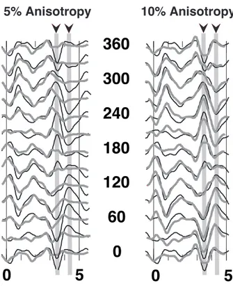
Seismic anisotropy in the upper mantle is known to be theoretically as large as 20%. However, no percentage of anisotropy larger than 5% is usually observed at upper mantle depths (e.g. Tommasi et al. (1999)). In this study our percentage of anisotropy vary between 8 and 12%, stronger than expected, but necessary to fit the pattern described by data. A conservative value for mantle anisotropy (5%) is not enough to produce the right phase amplitude (left panel of Figure 2.6). Conversely 10% of anisotropy gives a better fit to the waveform. Such high value is consistent with recent studies (Levin et al., 002b; Savage et al., 2007; Vinnik et al., 2007; Piana Agostinetti et al., 008a) and theoretical predictions (Blackman & Kendall, 2002).

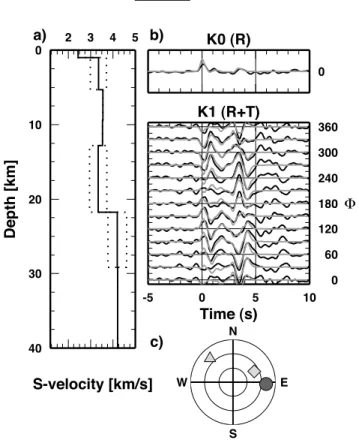
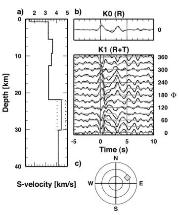
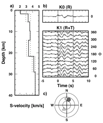
Figure 2.4: (a) Mean velocity model for station RDP. Solid line indicates S-velocity profile, while dotted lines enclose anisotropic layers. (b) K0 and K1 harmonic coefficent expansion (HCE) for station RDP. Observed HCE (black lines) are overplotted by synthetics HCE (grey). (c) Southern emispheric pro-jection of the 3D parameters for RDP model. Circle indicates trend and plunge of the symmetry axis in the upper crust anisotropic layer, triangle shows trend and plunge for the anisotropic layer in the lower crust, diamond shows trend and plunge of the upper mantle anisotropic layer.

2.4 Inversion Method 15 0 10 20 30 40 2 3 4 5 0 k0(R) N E S W -5 0 5 10 -5 0 5 10 k1 (R+T) -5 0 5 10 Time (s) 0 60 120 180 240 300 360 Φ S-velocity [km/s] -5 0 5 10 12 3 3 3 a) b) c) d) e) f) 4 5 4 5

Figure 2.5: (a) S-velocity models for station RDP, red model has no anisotropic layers, green model has only the upper crust anisotropic layer, blue model has the upper crust and the upper mantle anisotropic layers. (b) K0 diagram com-paring data and synthetics for the three models in panel (a): red, green and blue wiggles correspond to the the relative color model. (c) Southern emispheric pro-jection of the 3D parameters: circles indicate trend and plunge of the symmetry axis in the upper crust anisotropic layer, diamond shows trend and plunge of the upper mantle anisotropic layer. In panels (d), (e) and (f), K1 gathers comparing data (black) and synthetics (color) for the three models in panel (a).

0

60

120

180

240

300

360

0

5

0

5

5% Anisotropy

10% Anisotropy

Figure 2.6: Comparison for upper mantle anisotropy values. On the left, ob-served RF (black lines) and synthetics RF (grey) computed from a model with 5% of upper crustal anisotropy. On the right, the same but for a model with 10% of upper mantle anisotropy.

2.5 Results 17

2.4.3

Errors on layer thickness

We estimate the errors on the thickness of the layers by adding random noise to a synthetic RF data-set and comparing the resulting models with the input model (Figure 2.7) (Vinnik et al., 2004). In this case, both the input and the resulting models are performed for a 1D structure which is similar to the 1D S-velocity model computed for RDP. We assume a white gaussian noise in the RFs with a standard deviation of 0.25. We run the inversion in the same way of the real data; at the end of the search stage, we set a misfit threshold, i.e. 1.25 times the best-fit model misfit, and select all models in the ensemble which have the misfit lower than the threshold. We compute the variability of each inverted parameter as the min/max interval of the parameter in the selected family. We estimate the errors on the inverted parameters as the half-width of the intervals of variability of the parameters. This test allow us to define errors on thickness and depth: about 0.5 km for the shallow sediments thickness, 1 km for the limestones thickness, and 1.5 km for the Moho depth.

2.5

Results

We show and discuss the results of the 3D model inversion, with the aim of understanding the effects generated by the building of the volcanic edifice on undeformed crustal structure. To do that, we looked at results station by station focusing progressively on the volcano edifice, and we analysed the symmetry axes for each data-set. Also, trend and plunge of the symmetry axis detected in each anisotropic layer encountered are studied using the Bayesian approach and their PPD as shown in Figure 2.15.

Station AL08 is a reference for the regional structure surrounding the vol-cano, since it is located about 10 km to the NE of the caldera (see Figure 2.1) and close to the carbonate outcrops of the Apennines. For this station, the isotropic component of the harmonic analysis (K0) reveals a strong conversion at about 3.2 s, related to the Moho. The first harmonics (K1) shows two derivative pulses at about 0.5 and 3.5 s, with a polarity flip at about 60◦of Φ (φ=150 in Figure 2.8). The first feature indicates the existence of a shallow dipping interface. Since the Moho conversion occurs at 3.2s, the second feature is consistent with the presence of an anisotropic layer in the upper mantle. Consequently, our a priori information consists of a dipping interface between the first and second layers and a fast anisotropic layer underneath the Moho. The computed 3D model shows a thin sedimentary cover, ∼1 km thick, lying above a 5 km thick carbonate sequence (Vs3.3 km/s). Underneath the limestone layer, we observe very high S-wave velocities (3.6 km/s between 6 and 13 km depth), and a Vs reduction in the lower crust. The Moho is modelled at 22 km depth, and the sub-Moho anisotropic layer shows an axis trending N64◦_{, plunging 35}◦_.

Station AL01 is located on the western side of the volcano, about 6 km from the Albano lake. The K0 component presents a negative pulse at 1.5 s, followed by a positive pulse at 2.5 s, related to the conversion at the Moho. The K1 component shows a derivative pulse in the first second, with a polarity that reverses at φ=150◦and a second couple of pulses between 2.5 and 4 s. While the

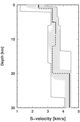
Figure 2.7: Estimating the standard error of inversion by numerical experiment. Solid blak line indicates the ”true” model, used to generate the ”observed” data-set. The grey area is composed of all the best-fit models selected from the entire sampled ensemble. The bounds for velocity are shown by thin dashed line, while a white dashed lines indicates the best-fit model.

2.5 Results 19

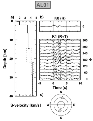
Figure 2.9: As in Figure 2.4, for station AL01.

former can be related to a shallow dipping discontinuity, the latter requires two anisotropic layers, in the lower crust and in the mantle. The anisotropic layer in the lower crust is needed to fit the data. In the uppermost crust, the 3D model shows a 0.5 km thick volcanic cover overlaying a ∼2 km thick Plio-Pleistocene sediment layer and a 4 km thick carbonate layer. Underneath the limestone, we find a small S-wave velocity jump between 7 and 15 km depth, consistent with the Pre-Mesozoic basement. In the lower crust, we find a 7 km thick anisotropic layer with high S-wave velocity, its axis trends N12◦ with a 32◦ plunge. In the uppermost mantle, beneath the Moho modelled at 22 km depth, a layer with a small anisotropy (3.9%) is observed oriented N194◦ plunging 41◦ (Figure 2.9).

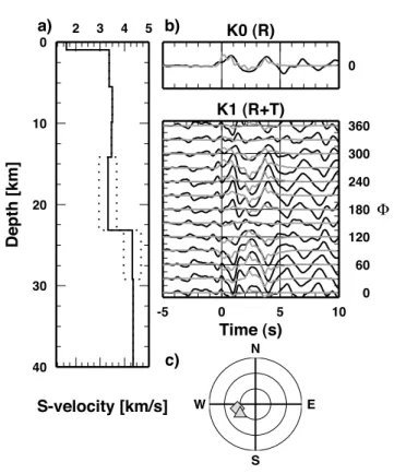
Station AL12 (Figure 2.10) is located to the south of the volcano on the carbonate units of the Lepini mountains. On the K0 component, we observe a clear pulse at 3 s, related to the Moho. The K1 component shows a couple of pulses flipping at about 120◦ _{(at 0.5-1 s), and two broad pulses at 3-4.5 s,} flipping at the same direction, interpreted by a shallow interface and two deep

2.5 Results 21

Figure 2.10: As in Figure 2.4, for station AL12.

anisotropic layers. The obtained crustal structure is simple: a 26 km thick crust with an almost constant S-wave velocity. The shallow interface coincides with the base of the carbonate layer, and shows a gentle dip towards SW. In the lower crust and uppermost mantle, we find two highly anisotropic layers, the first is oriented N245◦, plunging 55◦ the latter trends N219◦, plunging 25◦. These two layers are separated by the Moho modelled at 26 km depth.

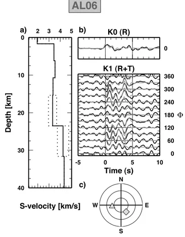
Station AL06 is located on the northern edge of the Tuscolano-Artemisio caldera ring (see Figure 2.1). The K0 component shows the Moho related pulse at 3.3 s. The K1 diagram shows three main couple of derivative pulses at 1, 2 s and between 3.5 and 5 s (Figure 2.11). We attribute the first couple to a shallow dipping layer and the two later pulses to anisotropic layers located above and below the Moho. The sharp pulses at 2 and 3.5 s strongly require the anisotropic layer in the lower crust. The 3D velocity model reveals a thick (2 km) layer of volcanic rocks overlaying a 5km thick carbonate sequence, separated by a 340◦-striking and 17◦ E-dipping interface probably indicating the top of the

Figure 2.11: As in Figure 2.4, for station AL06.

limestone. Anisotropy is revealed in the lower crust with N254◦ _{trending axis,} plunging 65◦_{, and an uppermost mantle with a N144}◦ _{oriented axis, plunging} 39◦. The Moho is modelled at 25 km depth.

Station AL09 is located a few kms to the north of station AL06 and similarly is featuring a shallow dipping interface and two deep anisotropic layers. Any-way, the trending of interfaces and anisotropy axes desumed by the harmonics analysis are different. In the K1 diagram (Figure2.12), we observe two pulses at 1-1.5 s (flipping at N330◦) due to the shallow dipping layer, and two pulses between 2.5 and 4 s, due to two anisotropic layers with the fast axes trending between N200◦and N300◦. The computed model shows a ∼1 km thick sediment layer lying above a 5 km thick limestone layer. The base of the limestone co-incides with the N128◦-striking, 35◦ W-dipping discontinuity. The lower crust has a N240◦_{-trending 55}◦ _{plunging anisotropy fast axis. The Moho is modelled} at 23 km depth, and the fast axis of anisotropy in the uppermost mantle is N256◦-trending and 54◦plunging.

2.5 Results 23

The three stations AL02, AL03 and RDP are located inside the Tuscolano Artemisio caldera, over the volcanic products related to the second and the final volcanic activity (see De Rita et al., 1995)

On K1 diagrams, stations AL02 and RDP show similar couple of pulses with the same arrival time, but with different directions of polarity inversion (Figures 2.13 and 2.4). We observe two coupled pulses in the first second, a single phase at 2 s, and two coupled pulses between the 3 and 4 s. The coupled pulse in the first second is only revealed at the stations inside the caldera and is due to a very shallow feature. In the uppermost few kms, the deep structure of the volcano is composed by volcanic rocks and Meso-Cenozoic limestone units (see Chiarabba et al., 1994). Therefore, we associate the coupled pulse to a shallow anisotropy derived from the layering of sedimentary rocks, preferential sites for magmatic intrusions. In this case, the anisotropy axis would be slow and perpendicular to the layering. While arrival times of the first couple are exactly the same for both stations, the polarity change occurs at N270◦and N30◦for AL02 and RDP, respectively. This sharp variation at very close stations suggests that both axes are pointing roughly towards the center of the volcano. The two other features are the lower crust and uppermost mantle anisotropic layers, features already observed for the other stations. Velocity models obtained for these two stations are similar. In AL02, we find two shallow layers related to the volcanic rocks and sediments (2 km thick) and to the limestones (4 km thick). The slow anisotropic axis trends N21◦ and plunges 54◦. The lower crust anisotropy fast axis is oriented N234◦and plunges 57◦. The Moho is located at 23 km, and the upper mantle anisotropic fast direction is N35◦, with a plunge of 29◦. In RDP, the sediment and volcanic layer is 1 km thick, the carbonate layer is 4 km thick and the slow anisotropic axis is oriented N93◦, with a plunge of 20◦. The lower crust anisotropic axis is N316◦_{with a plunge of 20}◦_{. The Moho is located at 21} km depth and the upper mantle fast anisotropy direction is N63◦, with a plunge of 40◦. Station AL03 is located 5-6 km to the southeast of AL02 and RDP. The harmonics analysis shows 5 pulses within the first and the fourth seconds. We associate the first couple of pulses to the shallow anisotropy already observed at AL02 and RDP. In AL03, its arrival time is slightly delayed (1 s) suggesting that the anisotropic layer is a few km deeper than for the two other stations. The a priori information for the modeling consists of three anisotropic layers, similarly to AL02 and RDP. The velocity model shows a 1 km thick sediment layer overalying 4 km thick limestones. The slow anisotropy axis, located at the base of the limestone layer, is N225◦ trending and 51◦ plunging. The fast axes have N336◦ and N194◦ with plunges of 30◦ and 47◦, for the lower crustal and uppermost mantle anisotropic layers, separated by the Moho located at 22 km. Figure 2.15 shows the Posterior Probability Distribution (PPD) for the anisotropic parameters estimated for each station. Well constrained parame-ters have a sharp Gaussian distribution. We observe that while the plunges of anisotropic axes have a broadened gaussian distribution, trends of anisotropic axes are generally well constrained; however some trend parameters are not well resolved, as for the lower layer of station AL01, AL02 and AL09. This happens because the shallowest layers, displaying a sharp gaussian, badly influence the resolution of the directions of deeper layers.

2.5 Results 25

2.5 Results 27

Figure 2.15: 1D posteriori probability density (PPD) function from Bayesian resampling. Here, only anisotropic parameters are reported (trend and plunge) for every anisotropic layer in the S-velocity profiles. Grey vertical lines indicate the mean of each distribution.

2.6

Discussion

Seismic wave velocity depends on several factors, including lithology, tempera-ture, stress, fabric, mineralogy, fluid inclusions, and pore properties and pressure (O’Connell & Budiansky, 1977; Kern, 1982; Mavko, 1980; Sato et al., 1989). In Quaternary volcanoes, the repeated accumulation of magma produces sharp and abrupt horizontal and vertical variations of P- and S-wave velocities. Seismo-logical techniques help to indirectly trace the location and geometry of magma conduits, solidified intrusions and magma chambers (Lees, 1992; Mori et al., 1996; Okubo et al., 1997; Chiarabba et al., 2004). In the Colli Albani, great ef-fort was spent in recovering the uppermost crustal structure with tomographic techniques (Chiarabba et al., 1994; Feuillet et al., 2004). High P-wave velocity anomalies are identified and related to the presence of shallow solidified mag-matic bodies nested within the limestone layer at 4-5 km depth. Since the last volcanic activity at the Colli Albani is older than 25 ka, and is volumetrically small, the crustal structure more likely reflects the older volcano activity, which was elevated between 600-200 ka (De Rita et al., 1995).

The inversion of RFs adds significant new information on the crustal struc-ture of the volcano and surrounding regions down to the uppermost mantle. The harmonics analysis points out that dipping discontinuities and anisotropy in the crust and upper mantle largely affect the RFs at the Colli Albani. Neglecting such 3D heterogeneities, the computation of an isotropic 1D S-wave velocity model may be severely biased (Christensen, 2004). Therefore, we computed 3D velocity models, inserting a priori the existence and the reasonable range for anisotropic parameters, and modelled contemporaneously the isotropic and anisotropic structure. The caveat is that 1D and 3D features are coupled on the RF and the modeling may be unbalanced towards either the isotropic or anisotropic parameters. We prefer to model at the best the 3D heterogeneities, leaving some small spurious discontinuities on the isotropic velocity profiles. Anyway, the robust isotropic features, i.e. the Moho and the top of the lime-stone layer, are well resolved and stable for all the stations. The existence of this coupling, undoubtfully present in complex tectonic structures, is rapidly emerging in RFs modeling, but still not completely addressed (Savage, 1998). We believe that our study provides new information for a more general use of RF in complex media. Our results shows that the Vs models define coherently the regional structure, featuring a thinned crust (21 to 26 km depth), shallow carbonate layers in the upper 6-8 km depth, and a general low Vs in the lower crust. In the shallow structure of the volcano (5-10 km depth), we do not ob-serve a Vsreduction ascribable to a crustal magma chamber or melt (Nakamichi et al., 2002). Conversely, we find a high Vsbody located underneath the lime-stone layer, probably referable to an old intrusion and cold solidified material of the former volcano activity (Lees, 1992). Such body may be the intrusive root of the high Vp body revealed by local earthquake tomography at shallower depth (Feuillet et al., 2004). Since the complexity of the shallow 3D features, we are not able to resolve the presence of tiny low Vsvolumes in the upper 15 km beneath the resurging area. If new magma was emplaced in the shallow crust during the unrest episodes, the last of which occurred in 1989-1990, the

2.6 Discussion 29

dimension of such bodies, nested within the high Vs old intrusion, should be small enough to be undetected by RF.

The most intriguing and innovative result is the recovering of strong anisotropic layers in the crust and uppermost mantle. The presence of seismic anisotropy is necessary to model the pulse variations on the R and T components ob-served in the RFs (Figures 2.8 to 2.14). Beneath the study region, we recognize three anisotropic layers (Figure 3.12). The shallow anisotropic layer changes in orientation even at close stations. It is present only at the three stations located within the caldera and became shallower moving towards the centre of the volcano. We attribute this feature to the layering of the sedimentary lime-stone pile, possibly alternated with intruded magma. For sedimentary rocks, the slow axis of anisotropy is perpendicular to the stratification (Sherrington et al., 2004). The conic-like pattern, radial to the volcano, suggests that the limestone layer was deformed by the up-welling of magma in the central cone. Remains of the solidified magma are traced between 5 and 10 km depth by the high Vs at the three stations. Alternatively, the 3D feature observed on the RF can be explained by two dipping interfaces coinciding with top and bottom of the limestone layer. Since the resulting geometry of the carbonate layer is inconsistent with the available geologic data (De Rita et al., 1988), we prefer the former interpretation. The second anisotropic layer is located in the lower crust (14-26 km depth) and is visible at almost all the stations. In the lower crust, seismic anisotropy is due to the alignment of minerals grains, metamor-phism, ductile deformation or crustal flow during tectonic events (Savage, 1999; Meissner et al., 2006). The percentage of anisotropy varies between 8 and 15% and the fast axis is sub-vertical (see Figures from 2.8 to 2.14), while the slow axis is almost sub-horizontal. Since the two different simmetry axes (fast and slow) generate the same feature on RF if oriented in opposite direction and plunging with a complementary angle, the choice of one or the other is abso-lutely arbitrary, as we show in section 3.1, and depends on crustal composition. In our results, we got direction for fast axes, but as showed in Figure 3.12 the slow associated axes for lower crust seems to fit better into the whole structure, arranging almost parallel to the fast axes detected in the upper mantle. This last anisotropic layer, located in the uppermost mantle below 25 km depth has a percentage of anisotropy of about 8-12% and is present at all the stations.

Although seismic anisotropy in the lower crust and uppermost mantle should be expected in case of a robust flux that aligns anisotropic minerals (biotite, amphibolite, granulite, olivine), evidence and measurements from seismological data are still poor. Recently, RF modelling showed the existence of several anisotropic layers in the lower crust in the Tibet region (see Sherrington et al., 2004). The presence of such high anisotropy percentage in the mantle is striking, but reliable as demonstrated in section 4.2.2).

In Figure 2.17 we show a comprehensive sketch of our results. Sediments cover the entire area buring the limestones layer. The high velocities under the limestones are interpreted (where present) as the Triassic anydrites constitu-ing the basement of the Mesozoic sequence. These two latter layers probably are locally deformed by the magma intrusion, and their tilt is the cause of the observed seismic anisotropy. This is in agreement with previous studies in

12°30’E 13°00’E 12°30’E 13°00’E 41°36’N 41°48’N 0 4 8

km

Upper ani (Slow) sym. axis Middle ani (Fast) sym. axis Middle ani (Slow) sym. axis Lower ani (Fast) sym. axis

0 10 20 30 40 0 10 20 30 40 -20 -15 -10 -5 0 5 10 15 20 Depth [km] A A' 0 500 1000 0 500 1000 Alt [m] AL01 AL02 RDP AL03 AL06 AL08 AL09 AL12 0 10 20 30 40 0 10 20 30 40 -20 -15 -10 -5 0 5 10 15 20 Depth [km] B B' 0 500 1000 0 500 1000 Alt [m] AL01 AL02 RDP AL03 AL06 AL08 AL09 AL12 0 10 20 30 40 0 10 20 30 40 -20 -15 -10 -5 0 5 10 15 20 Depth [km]

Distance along profile [km]

B B' 0 500 1000 0 500 1000 Alt [m] AL01 AL02 RDP AL03 AL06 AL08 AL09 AL12 A) B) C)

Figure 2.16: Map of the studied region, showing anisotropy axes direction (blue arrows) for the upper crust, and profiles AA’ and BB’ traces. (A) AA’ and (B) BB’ profiles showing distribution of symmetry axes in each anisotropic layer; color coding is: blue for the upper crust, yellow for the lower crust, and red for the upper mantle. (C) BB’ profile, as for BB’ in (B), but the green arrows indicate slow-axis in lower crust anisotropic layers.

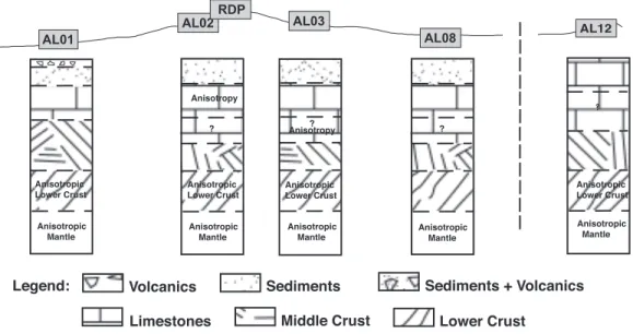
2.6 Discussion 31 ? ? v v v v v v v v v v v v v v v v v v v v v v v v v v v v v v v v v v v v v v v v v v v v v v v v v v v v v v v v v v v v v v v v v v v v v v v v v v v v v v v v v v v v v v v v v v v v v v v v v v v v v v v v v v v v v v v v v v v v v v v v v v v v v v v v v v v v v v v v v v v v v v v v v v v v v v v v v v v v v v vv vv v v v v v v v v v v v v v v v Legend: v v v v v v v v v v AL02 RDP AL03 AL08 AL01 Moho Sediments Volcanics Limestones

Anydrites Middle Crust Lower crust Magmatic Intrusions Mantle Flux Sediments + Volcanics

Figure 2.17: Summary sketch of results. Stations are projected on the AA’ profile of Figure 3.12. Seismic anisotropy with negative slow simmetry axis is considered in lower crust, as in Figure 3.12c.

which the magmatic chamber was identified as a high Vp body at 5-6 km depth (Chiarabba et al., 1997; Feuillet et al., 2004).

The middle crust does not show any particular characteristic, while the lower crust and the upper mantle are characterised by strong anisotropy in which the symmetry axes distribution suggest that it is generated by localized deformation manifested in fossil fabrics. Three main tectonic events can reasonably have produced such fossil fabric: the Mesozoic extension related to the opening of the Tethys ocean, the Cenozoic compression that build up the Apennines and the more recent extension of the Tyrrhenian back arc region. During this last event, the pervasive extension in the Tyrrhenian plate, induced by the Apennines slab rollback (Gueguen et al., 1998), re-organized the flow in the mantle wedge. In such case, a consistent sub-horizontal direction perpendicular to the slab edge should be expected, except in the corner flow region, and we do not observe a defined horizontal alignment of simmetry axes. We favour the interpretation of a sub-vertical flux in the mantle coherent with the magma up-rise from a mantle source located below 30 km depth. This flux, vigorous in the past 1-2 Ma, aligned the direction of mineral crystallographic axes in the mantle and in the lower crust. More speculatively, the variation of the plunge of fast axes, moving away from the volcano, suggests that the flux of magma followed local small-sized convective cells. At a local scale, the magma upraise beneath this volcano is mirroring the mantle flow of plate tectonics.

2.7

Conclusions

The analysis and modeling of teleseismic receiver functions helps to understand the crustal and upper mantle structure beneath the Colli Albani Quaternary volcano in central Italy. The 3D S-velocity models are consistent with the regional structure of the Tyrrhenian. Most robust features are: (1) limestones are present as remnants of the Mesozoic platform, they have thickness between 4 and 5 km. Their structure is plane, and for the stations under the calderic edifice they present a clear and well defined anisotropic pattern as on Figure 3.12; the slow anisotropic axes evidence a volcanic-related structure; (2) a high Vsvalue for the under-carbonates layer is recognised, this can be due to cold intrusive accumulated material. (3) a shallow Moho, present at depths between 21 and 26 km, as evidence of a thinned crust. (4) lower crust and an uppermost mantle in all the stations considered in this study show distinct anisotropic patterns. These are generated probably by the local flux of the ascended magma. This area is also involved in tectonic processes of back-ark extension, so fossil or active structures are deepely conditioned by both processes generating anisotropy.

CHAPTER

THREE

Mapping seismic anisotropy using harmonic

decomposition of Receiver Functions: an application to

Northern Apennines, Italy.

Isotropic and anisotropic seismic structures across Northern Apennines (Italy) subduction zone are imaged using a new method for the analysis of teleseismc receiver functions (RFs). More than 13,000 P-wave coda of teleseismic records from the 2003-2007 RETREAT experiment are able to reveal new insights into a peculiar subduction zone which develops at the convergent margin of two conti-nental plates and is considered a focal point inside the Mediterranean evolution. A new methodology for the analysis of receiver function is developed, which combines both migration and harmonic decomposition of the receiver function data-set. While migration technique follows a classical “Common Conversion Point” scheme and helps to focus on a crucial depth range (20-70 km) where mantle wedge develops, harmonic decomposition of a recevier function data-set is a novel and less explored approach to the analysis of P -to-S converted phases. The separation of the back-azimuth harmonics is achieved through a numeri-cal regression of the stacked radial and transverse receiver function from which we obtain independent constraints on both isotropic and anisotropic seismic structures. The application of our new method to RETREAT data-set succeeds both to confirm previous knowledge about seismic structure in the area and to highlight new structures beneath the Northern Apennines chain, where previ-ous studies failed to clearly retrieve the geometry of the subducted interfaces. We present our results in closely spaced profiles across and along the Northern Apennines chain to highlight the presence of the Tyrrhenian and the Adriatic side which differ in the thickness of the crust (about 25 km the first one, and about 40 km the second one). These two plates converge in the central zone where the Adriatic plate subducts beneath the Tyrrhenian. A signature of the dipping Adriatic Moho is clearly observed beneath the Tyrrhenian Moho in a large portion of the forearc region. In the area where the two Mohos overlap, our new analysis reveals the presence of an anisotropic body above the subducted Moho. There is a strong Ps converted phase with anisotropic characteristics

from the top of the Adriatic plate to a depth of at least 80 km. Because the Ps conversion occurs much deeper than similar Ps phases in Cascadia and Japan, dehydration of oceanic crust seems unlikely as a causative factor. Rather, the existence of this body trapped between the two interfaces supports the hypoth-esis of lower crustal delamination in a post-subduction tectonic setting.

3.1

Introduction

Developed between the European plate and the continental Adriatic microplate, the Northern Apennines (NA) are characterized by an active accretionary wedge that is actually below sea-level in central Adriatic but contains active thrust faults at the southern border of the Po River Valley (Picotti & Pazzaglia, 2008; Wilson et al., 2009) and the elevated area is both in uplift and extension (Figure 3.1). Deep earthquakes occur along some portions of the NA chain, reaching maximum depths of about 90 km (De Luca et al., 2009). Tomographic studies reveal the presence of a westward dipping fast anomaly beneath the NA area, suggesting the sinking of a cold body into the mantle (Lucente et al., 1999). Re-gional tomographic results suggest thinner crust in the Tyrrhenian side than in the Adriatic one, associated with a small velocity jump at the Moho (Di Stefano et al., 2009). Low-seismic velocity in the uppermost mantle under Tuscany has also been suggested from surface wave studies (Levin & Park, 2009). Measures of SKS splitting in the area highlight a complex link between mantle flow under the NA and orogenic evolution (Salimbeni et al., 2008). An eastward retreating slab has been invoked as principal driving process in this area (Malinverno & Ryan, 1986), able also to describe the present position of the orogen, but hy-potheses have been argued where this motion is a steady-state (Faccenna et al., 2004), or ongoing process (Doglioni, 1991).

Receiver Function (RF) analysis is a widely applied technique that uses P -to-S converted waves, generated at sub-surface seismic discontinuities, to map sharp lithologic contrasts at depth. Receiver functions are based on two simple assumptions. First, a plane P-wave which crosses a planar seismic disconti-nuity is (partially) converted to an S-wave. Second, for teleseismic P waves, source and path effects are recorded on the vertical Z component of the seis-mograms. Thus, a simple deconvolution of the horizontal components from the vertical gives rise to two time-series, a radial (Q-RF) and a transverse (T-RF), which contains the P -to-S converted waves beneath the receiver (Vinnik, 1977; Langston, 1979; Levin & Park, 1998; Savage, 1998). The Q-RF contains energy mainly from the isotropic seismic structure beneath the receiver, while TRF carries information primarily from the anisotropic and/or dipping subsurface structure. Q-RF analysis has been widely used to create images of subduction zones (Ferris et al., 2003; Bannister et al., 2007; Kawakatsu & Watada, 2007; Piana Agostinetti et al., 2009). Analysis of the energy on the TRF data-set is far less common. A large TRF data-set from a single seismic station has been used to image both anisotropic and dipping structures beneath the receiver (Savage, 1998; Park et al., 2004; Piana Agostinetti et al., 008c). Harmonics coefficent analysis, involving both Q- and T- RF, has been developed for the analysis of

3.1 Introduction 35 8˚ 8˚ 10˚ 10˚ 12˚ 12˚ 14˚ 14˚ 42˚ 42˚ 44˚ 44˚ 46˚ 46˚ 100 km Elba Island Po Plain Tyrrhenian Sea Tuscany Adriatic Sea Ligurian Sea 7 mm/year convergence

Figure 3.1: Tectonic sketch fo the study area. Main tectonic boundaries are displayed outlining areas affected by compression and extension. The arrow indicate the convergence direction between Eurasia and Africa plate, almost parallel to the development of the compression/extension area.

subsurface anisotropy (Girardin & Farra, 1998; Bianchi et al., 2008) under iso-lated seismic stations. However, few imaging techniques, which use data from several seismic stations, join the analysis of the Q- and T- RF data-set (Tibi et al., 2008; Mercier et al., 2008; Tonegawa et al., 2008).

RF techniques have been applied to study the NA area. Moho depth in NA region has been estimated using both temporary (Piana Agostinetti et al., 2002) and permanent (Piana Agostinetti & Amato, 2009) seismic stations. A selection of the RETREAT data-set has been employed to estimate crustal properties, i.e. thickness and VP/VS, across the NA chain, using a simple grid-search approach (Piana Agostinetti et al., 008a). The anisotropic seismic structure of the forearc Adriatic crust has been studied in Levin et al. (002a), while Roselli et al. (2010) investigated both isotropic and anisotropic structure of the Tyrrhenian crust in the fore-arc. Strong evidence of heterogeneity in the crust and upper mantle has been detected (Piana Agostinetti et al., 008a) under the NA chain, where the previous studies failed to clearly reveal the geometry of the subducted interfaces. In this study, we apply a new technique for RF analysis which allows the sep-aration of the back-azimuth harmonics of the Q- and T- receiver-function data-set as a function of the incoming wave-field direction. Energy due to anisotropic and/or dipping subsurface structures is separated from the isotropic signals, and partitioned in 2-lobed back-azimuth harmonics, cos φ and sin φ, which become the principal tool for the understanding of subsurface geometries. Data are stacked along profiles which image both isotropic and anisotropic structures. The input data for the profiles are obtained by a Common Convertion Point (Dueker & Sheehan, 1998) stack technique to focus our analysis between 20 and 70 km depth. In this chapter, we first describe the harmonic decomposition and the migration methods. Then, we present results from the analysis of the RE-TREAT data-set, and we discuss our method and the geodynamics implications of the results.

3.2

Data & Method

We use a dataset composed of about 13, 000 RFs obtained from teleseismic records occurred at epicentral distance between 30◦ and 100◦, and with M > 5.5, and selected by their high signal-to-noise ratio. Teleseismic events were recorded at 51 broadband, 3-component stations, deployed along peninsular Italy, between 42◦N and 46◦N (Figure 3.2). Forty stations were operating by RETREAT experiment for three years (10/2003 to 09/2006) (Margheriti et al., 2006).Ten stations are permanent seismic observatories of the Italian National Seismic network; and one station (VLC) belongs to the Mediterranean Network (MedNET). All stations recorded continuously between 2003 and 2006. Due to the long working period of the RETREAT array, we obtain a good back-azimuth coverage (Figure 3.3).

Seismic records are rotated into the LQT reference system to enhance the converted P s phases. L is the direction of the hypothetical incoming P wave (computed using IASPEI91 model) and Q is perpendicular to L in the vertical-radial plane, i.e. the plane that contains source and receiver. T is normal to

3.2 Data & Method 37 10˚ 10˚ 12˚ 12˚ 14˚ 14˚ 42˚ 42˚ 44˚ 44˚ 50 km A A’ B B’ C C’ D D’ E E’ ELBR ELBR RAVR RAVR 14 20 17

Figure 3.2: Map displaying stations (black triangles); piercing points (grey crosses) at 40 km depths for the events recorded at stations and used in this this study. The map shows also the locations of 5 profiles, white dots represent the spots for which we estimated a RF along profile directions. Spots 14, 17 and 20 in profile BB0 are represented by stars. ELBR and RAVR stations (at the beginning and end of BB0) are displayed.

0˚ 45˚ 90˚ 135˚ 180˚ 225˚ 270˚ 315˚ 25 50 100 N S E W

Figure 3.3: Black stars represent the location of teleseismic events recorded at Spot 17 in profile BB0. Numbers indicate back-azimuth φ (rays) and epicentral distance ∆ (circles).

the L-Q plane. Receiver functions are calculated by frequency-domain inversion algorithm using multi-taper correlation estimate (Park & Levin, 2000). We use a frequency cut-off of 0.5 Hz, which gives us a vertical resolution of approximately 3 − 5km.

3.2.1

CCP and Migration

To enhance the continuity of the structures in the study area, we implemented a Common Convertion Point technique (Dueker & Sheehan, 1998; Wilson et al., 2004) (see also Supporting Material). We select five main profiles across North-ern Apennines (Figure 3.2). Three profiles (AA0, BB0and CC0) share the same direction N18◦E approximately orthogonal to the strike of the Apennines oro-gen (in its northern part, between 9◦E and 13◦E longitude). Two profiles (DD0 and EE0) are orogen-parallel. For each profile, we divide the area within 40 km of the profile into rectangular boxes 20 km wide, with a 50% overlapping scheme (i.e. each area shares 50% of its surface with the adjacent areas). For each rectangular area, we select the ensemble of RFs (both Q and T) for which the surface projections of their conversion points at a fixed migration depth fall inside the rectangular area. We associate the RF with the center of the rectangular area (the ’spot’, hereinafter). For our purpose, we migrate each RF using IASPEI91 model to 40 km depth (Figure S1). For each spot, we ob-tain an ensemble of Q-RF and T-RF which can be used to image the seismic