2021-01-07T15:49:17Z
Acceptance in OA@INAF
ARGOS at the LBT. Binocular laser guided ground-layer adaptive optics
Title
Rabien, S.; Angel, R.; Barl, L.; Beckmann, U.; BUSONI, LORENZO; et al.
Authors
10.1051/0004-6361/201833716
DOI
http://hdl.handle.net/20.500.12386/29573
Handle
ASTRONOMY & ASTROPHYSICS
Journal
621
Number
https://doi.org/10.1051/0004-6361/201833716 c ESO 2018
Astronomy
&
Astrophysics
ARGOS at the LBT
Binocular laser guided ground-layer adaptive optics
S. Rabien
1, R. Angel
7, L. Barl
1, U. Beckmann
6, L. Busoni
2, S. Belli
1, M. Bonaglia
2, J. Borelli
3, J. Brynnel
8,5,
P. Buschkamp
1, A. Cardwell
8, A. Contursi
1, C. Connot
6, R. Davies
1, M. Deysenroth
1, O. Durney
7, F. Eisenhauer
1,
M. Elberich
6, S. Esposito
2, B. Frye
7, W. Gaessler
3, V. Gasho
7, H. Gemperlein
1, R. Genzel
1, I. Y. Georgiev
3,
R. Green
8,7, M. Hart
7, C. Kohlmann
1, M. Kulas
3, M. Lefebvre
8, T. Mazzoni
2, J. Noenickx
7, G. Orban de Xivry
1,10,
T. Ott
1, D. Peter
3, A. Puglisi
2, Y. Qin
7, A. Quirrenbach
4, W. Raab
1,9, M. Rademacher
7, G. Rahmer
8,
M. Rosensteiner
1, H.W. Rix
3, P. Salinari
2, C. Schwab
4, A. Sivitilli
3, M. Steinmetz
5, J. Storm
5, C. Veillet
8,
G. Weigelt
6, and J. Ziegleder
11 Max-Planck-Institut für extraterrestrische Physik, Giessenbachstr., Garching, Germany
e-mail: [email protected]
2 INAF Osservatorio Astrofisico di Arcetri, Florence, Italy
3 Max-Planck-Institut für Astronomie, Königstuhl 17, Heidelberg, Germany 4 Landesternwarte, Königstuhl 12, Heidelberg, Germany
5 Leibniz-Institut für Astrophysik Potsdam (AIP), An der Sternwarte 16, Potsdam, Germany 6 Max Planck Institut für Radioastronomie, Auf dem Hügel 69, Bonn, Germany
7 Steward Observatory, 933 North Cherry Avenue, University of Arizona, Tucson, AZ, USA 8 Large Binocular Telescope Observatory, 933 North Cherry Avenue, Tucson, AZ, USA 9 European Space Agency – ESTEC, Keplerlaan 1, Noordwijk, The Netherlands
10 Space sciences, Technologies and Astrophysics Research (STAR) Institute Université de Liège, Belgium
Received 25 June 2018/ Accepted 19 October 2018
ABSTRACT
Having completed its commissioning phase, the Advanced Rayleigh guided Ground-layer adaptive Optics System (ARGOS) facility is coming online for scientific observations at the Large Binocular Telescope (LBT). With six Rayleigh laser guide stars in two con-stellations and the corresponding wavefront sensing, ARGOS corrects the ground-layer distortions for both LBT 8.4 m eyes with their adaptive secondary mirrors. Under regular observing conditions, this set-up delivers a point spread function (PSF) size reduction by a factor of 2–3 compared to a seeing-limited operation. With the two LUCI infrared imaging and multi-object spectroscopy instruments receiving the corrected images, observations in the near-infrared can be performed at high spatial and spectral resolution. We discuss the final ARGOS technical set-up and the adaptive optics performance. We show that imaging cases with ground-layer adaptive op-tics (GLAO) are enhancing several scientific programmes, from cluster colour magnitude diagrams and Milky Way embedded star formation, to nuclei of nearby galaxies or extragalactic lensing fields. In the unique combination of ARGOS with the multi-object near-infrared spectroscopy available in LUCI over a 4 × 4 arcmin field of view, the first scientific observations have been performed on local and high-z objects. Those high spatial and spectral resolution observations demonstrate the capabilities now at hand with ARGOS at the LBT.
Key words. instrumentation: adaptive optics – instrumentation: high angular resolution – instrumentation: spectrographs – gravitational lensing: strong
1. Introduction
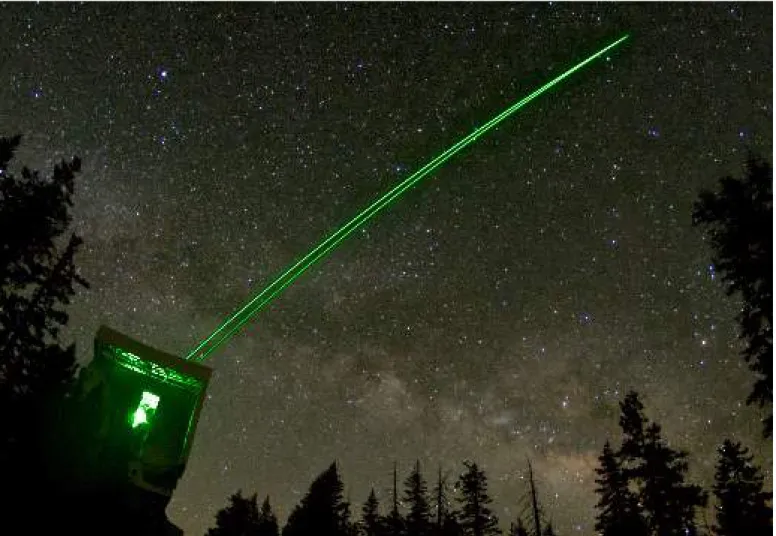
The Advanced Rayleigh guided Ground-layer adaptive Optics System (ARGOS) has been implemented to deliver a ground-layer adaptive optics (GLAO) correction to both of the 8.4 m “eyes” of the Large Binocular Telescope (LBT). GLAO is a tech-nique used to correct the atmospheric induced optical distortions over a large field of view, enhancing the image quality homoge-nously. To conduct this correction, ARGOS utilizes two con-stellations of multiple guide stars, generated artificially above the LBT with Rayleigh backscattering of high-power pulsed green lasers. Figure1shows the ARGOS binocular laser beams when propagated to sky. With range-gated wavefront sensing systems for the laser beacons and the LBT’s adaptive secondary
mirrors, the correction yields an improved point spread function (PSF) for imaging and spectroscopic observations. Enhancing the image quality with GLAO has several advantages. Increas-ing the spatial resolution gives insights into the details of an object’s structure. Additionally, the signal-to-noise ratio (S/N) in spectroscopy benefits strongly from sharpening the image. With the required integration time to reach a given S/N being inversely proportional to the square of the PSF diameter, obser-vations can be carried out in a much shorter time. Due to the smaller PSF size the spectroscopic slit width can be decreased accordingly, enhancing the spectral resolution and allowing spa-tially resolved spectroscopic observations. With GLAO deliv-ering a wide field-of-view correction, science cases benefit from adaptive optics that cannot be done with single-conjugate
Fig. 1.The ARGOS system propagating a bundle of laser beams on each side of the large binocular telescope. This wide-angle photograph was taken in 2017 with a 25 s exposure time. Each visible green beam in this image consists of three individual laser rays forming the wide-field constellations of guide stars in the atmosphere. The light pulses from the high-power lasers are subject to Rayleigh scattering by air molecules in the Earth’s atmosphere. Having the wavefront sensors gated and adjusted to receive the photons only from a distance of 12 km, a sharp reference beacon constellation is formed. Measuring the wavefronts and correcting the atmospheric ground-layer distortions with the two adaptive secondary mirrors yields a wide-field correction for imaging and spectroscopy.
systems or in seeing-limited mode. With a factor 2–3 PSF size reduction, ARGOS can be considered a “seeing enhancer” ben-eficial for the two facility instruments LUCI1 and LUCI2 o ffer-ing imagffer-ing and multi-object spectroscopy (MOS) in the near-infrared (NIR) wavelength regime. A multitude of science cases will benefit from the enhanced resolution and encircled energy that ARGOS delivers. Amongst others, scientific topics that can be addressed with the aid of GLAO span a wide range, from extragalactic cases such as high-z galaxy dynamics, active galac-tic nuclei, and Quasar host galaxies, to Galacgalac-tic astrophysical questions about planets, Cepheids, or stellar clusters. To summa-rize briefly, ARGOS with LUCI at the LBT offers the following benefits:
– Binocular observations, using the two 8.4 m telescopes of LBT at once;
– GLAO correction with a 0.200–0.300 resolution over a
4x4 arcmin field of view at both telescopes;
– A fairly homogeneous PSF shape over this full field (see Sect.3);
– A large 2 × 3 arcmin field for the tilt star selection;
– NIR imaging of the full field at the GLAO spatial resolution; – GLAO corrected NIR multi-object spectroscopy with custom
cut slit masks and high spectral resolution.
The last point emphasizes one of the unique capabilities that ARGOS provides. Currently this combination is only available at the LBT, enabling spectroscopic observations at high spatial and spectral resolution with slits cut to the object’s shape. The high spatial resolution allows the spectroscopic slits to be cut as narrow as 0.2500–0.300, pushing the spectral resolution up to R ∼ 10 000, enabling the detection of structures in the velocity distribution of high-z galaxies in great detail, and reducing the fraction of atmospheric bands for which the spectra are disturbed by the OH night sky emission lines.
In Sect. 2 we describe the ARGOS laser guide star (LGS) and adaptive optics system, now operational at the LBT. We give an overview of how the system is assembled, describe the laser beacon generation, the wavefront sensor units and its adaptive optics correction system. At the end of commissioning we can now show the resulting performance of the ARGOS binocular GLAO system. The analysis of the adaptive optics performance and the achieved image quality in the J, H, and K bands is dis-cussed in Sect.3. Having targeted a variety of objects in imag-ing and spectroscopic mode over the commissionimag-ing period, we can show selected science cases which highlight the capabilities of the system. Section4shows imaging programmes that bene-fit from the PSF size reduction: the globular cluster NGC 2419; the nearby galaxy NGC 6384, which hosts a massive nuclear star
Fig. 2. Sketch of the basic geometry of the GLAO scheme with the six laser beacons serving as reference for the adaptive optics. Located at a finite height above the telescope, the light from the laser beacons travels down on a cone through the Earth’s atmosphere. Turbulent layers located close to the ground will be sampled equally by all three beacons on each side, while on the high layers the footprints are completely separated and smaller than the illumination from the science object at infinity. The wavefront measurements from the high layers will average out over time, and the adaptive optics correction therefore is strongest for turbulent layers close to the ground.
cluster and a black hole; and three lensing galaxy clusters. In par-ticular, PLCK G165.7+67.0 (G165) ARGOS-corrected K-band imaging complementing HST WFC3/IR data allows us to detect the counter-image of one of the gravitationally lensed sources. One of the most powerful properties of ARGOS at the LBT is the combination of the custom cut slit masks in the LUCI spectrographs with the light concentrating GLAO system. We present curved slit spectroscopic observations of gravitationally lensed high-redshift galaxies which follows the long axis of the arcs. These spectroscopic programmes are focused on the “8 o’clock arc” and SDSS 1038+4849, which reveal structures within the interstellar medium of these systems undetected by other methods.
2. The ARGOS GLAO system
Within the multiple flavours of adaptive optics, the single-conjugate adaptive optics (SCAO) with sodium layer LGS is currently standard equipment at many large ground-based tele-scopes. The ESO UT4 (Lewis et al. 2014; Rabien et al. 2003), the Keck (van Dam et al. 2006; Wizinowich et al. 2006), or Gemini telescopes (Boccas et al. 2006) offer facilities of this kind. Since SCAO mainly corrects the column of turbulence in the direction of the guide star the usable field of view is lim-ited by the angular anisoplanatism to a ∼3000 patch. In order
to extend the suitable field of view, it is possible to imple-ment multi-conjugate adaptive optics (MCAO) with multiple guide stars and multiple deformable mirrors. Systems with this technique utilizing natural guide stars (NGSs) include the MAD test system (Marchetti et al. 2007) and LINC-NIRVANA (Herbst et al. 2016) at the LBT. GEMS at the Gemini south tele-scope (Rigaut et al. 2014;Neichel et al. 2014) is a MCAO sys-tem based on a sodium layer LGS constellation.
Proposed by Rigaut (2002), GLAO utilizes a single deformable mirror for the correction of the distortions located in the lower atmosphere, measured on multiple guide stars over a larger field. Natural guide stars can be used as reference sources, but many fields will not offer enough bright stars in a proper con-stellation to serve as adaptive optics probes. Laser guide stars are a natural choice for the wavefront measurement, offering a bright reference at the location of choice and constant posi-tions for repeatable results. Successful realizaposi-tions and tests of GLAO with Rayleigh lasers at smaller telescopes have been done at SOAR (Tokovinin et al. 2008), the WHT (Morris et al. 2004), and at the MMT (Hart et al. 2010).
The basic geometry of a GLAO system is shown in Fig.2. The constellation of laser beacons is placed at a finite dis-tance above the telescope. Therefore, the guide star light trav-els downwards through the atmosphere forming a “cone” on its path. Due to this geometry, the high-layer footprints of the beams are small and the constellations measurements will aver-age over time, leaving the ground layer as the only common sig-nificant contribution for the AO correction. As has been shown in several studies (e.g. Avila et al. 1998; García-Lorenzo et al. 2007;Tokovinin et al. 2005; Dali Ali et al. 2010), and in mea-surements at Mt. Graham (Masciadri et al. 2010), the vertical atmospheric turbulence distribution often shows a prominent ground layer, allowing GLAO to remove most of the distortions. The favourable property originating from the ground-conjugate geometry is the wide field of view where the correction is effec-tive. Placing the guide star constellation at a 4 arcmin diame-ter circle corrects a similarly sized field for the science obser-vation. The LUCI1 and LUCI2 instruments (Seifert et al. 2003; Buschkamp et al. 2012) cover this 4 arcmin field for imaging and MOS spectroscopy. Having been designed as an adaptive tele-scope from the beginning, the LBT (Hill 2010) is equipped with adaptive secondary mirrors on both sides (Riccardi et al. 2010). Since the Gregorian telescope has the adaptive mirror conjugated close to the ground at ∼100 m above the primary and the wide-field LUCI’s as receiving instruments, the choice for GLAO was obvious. ARGOS saw the first laser light on sky in November 2013 (Rabien et al. 2014) and the adaptive optics loop running successfully in early 2015 (Orban de Xivry et al. 2015). Now that commissioning is coming to an end, the 8.4 m apertures of the LBT are both equipped with an operational LGS-based GLAO system.
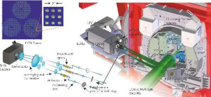
2.1. System description
ARGOS is based on constellations of laser beacons created by Rayleigh scattering from air molecules with multiple high-power pulsed green lasers. Upon a trigger command, all six laser heads fire synchronously the ∼40 ns light pulses. As they travel through the optical train of the laser systems and the launch telescope the beams are shaped, expanded, and focused at a distance of 12 km. While propagating through the Earth’s atmosphere, some pho-tons out of each pulse are scattered backwards by air molecules, given the well-known Rayleigh cross section. After 80 µs, pho-tons scattered at a distance of 12 km arrive back again at the
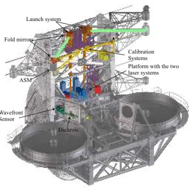
Fig. 3.Overview of the ARGOS components as installed at the LBT. The laser units are located in the centre piece between the two mir-rors on a dedicated platform. Leaving the laser systems, the beams are expanded with a refractive beam expander built into the LBT structure. The beams are directed behind the secondary mirror and sent to the sky by large flat mirrors. On the return path the photons are split off with a large dichroic mirror, which sends the light to the wavefront sen-sor. Calibration light sources and optics mounted on swing arms can be moved into the Gregorian prime focus for the adaptive optics calibra-tion. A total of eight electronics racks host the required infrastructure of drivers, readout, and controllers.
telescope and are detected by the wavefront sensor. In front of the instrument rotator structure we separate these photons with a dichroic beam splitter and direct the light towards the LGS wave-front sensors (LGSW). Inside these LGSWs the beams are first collimated before being sent through the Pockels cells gating units. These optical shutters are driven with a fast high-voltage switch to slice out exactly the photons scattered at 12 km within a selectable range, which is usually set to 300 m. The light out of this limited volume then propagates through the lenslet array onto the wavefront sensor detector. The detector itself is a fast, large frame PnCCD (Hartmann et al. 2008) allowing all three LGSs to be imaged on a single frame. In terms of timing, the lasers and Pockels cells are triggered at a 10 kHz repetition rate and the detector accumulates the photons from ten pulses before being read out, thus delivering a 1 kHz frame rate. The frames from the CCD are then transferred to the ARGOS slope basic computational unit (BCU). This computer calculates the cen-troid position of all spots and sends the resulting slope vector to the adaptive secondary mirror where the reconstruction is per-formed in dedicated fast parallel computers, and the thin shell of the adaptive secondary mirror is set.
Since the LGS position as measured on sky does not reflect the atmospheric tilt properly, a separate NGS tip-tilt sensor is required. For this purpose ARGOS can use either its own avalanche photo-diode quad cell (APD-QC) set-up, or the First Light AO (FLAO) pyramid sensor (Esposito et al. 2011,2010). While the APD system can detect fainter stars, the usage of the FLAO pyramid has proved to be more convenient during oper-ation. Indeed, the pyramid wavefront sensor is used to sense
Table 1. The parameters of the ARGOS main system.
Laser beacons per LBT side 3
Laser beacon gating height 12 km
Average power per laser 18 W
Laser repetition rate 10 kHz
Laser beam quality M2 <1.2
Launch beam diameter at e12 300 mm
Wavefront sensor frame rate 1 kHz
Number of sub-apertures across primary 15 × 15
Nominal range gating time 2 µs
Nominal LGS photon flux on the WFS∗ 5.8 × 10⁶m−2s−1 Notes.(∗)This number includes an optical round trip efficiency of 25%.
the “true” values for 21 low-order wavefront modes and slowly offset the LGS wavefront slopes. Its usage as tilt sensor addi-tionally avoids a complicated calibration of the APDs individual gains. The purpose of the truth sensing is to correct for non-common path aberrations, imperfect calibrations and the slight difference between elongated spots on sky and round calibration spots. ARGOS components are widely distributed over the tele-scope as can be seen in Fig.3. Apart from the core units of the two laser boxes, the launch expanders and the wavefront sensors being described in this paper, the system relies on a multitude of auxiliary units to be functional:
– A calibration system for each side mounted on swing arms (Schwab et al. 2010). This unit based on computer-generated holograms (CGHs) delivers light sources mimicking the far off-axis LGSs and a single NGS on sky in the Gregorian prime focus;
– A laser alignment telescope system to detect the initial loca-tions of the lasers on sky and automatically adjust the posi-tion (Sivitili 2016);
– The high-speed slope computing units (Biasi et al. 2004) based on a field programmable gate arrays system;
– A vibration compensation system based on accelerometers and fast laser uplink stabilization (Peter et al. 2012); – Transponder-Based Aircraft Avoidance (TBAD), the aircraft
detection units for an operation without human aircraft spot-ters (Rahmer et al. 2014);
– An infrastructure of drivers, controllers, cameras, computing units, safety systems, etc., filling eight electronics racks at the telescope.
The ARGOS main system parameters are listed in Table1. 2.2. Creating the laser beacons
Although the very early LGS systems already used Rayleigh scattering of high-power laser beams for the creation of the bea-cons (see e.g.Fugate et al. 1991;Parenti 1992), this method has become less popular since the adoption of sodium layer beacons. Beacons created in the sodium layer are at much higher altitude; therefore, the focal anisoplanatism is less problematic with this method. Nevertheless Rayleigh beacons offer several advantages over sodium beacons, making them very attractive:
– Rayleigh backscatter yields a high photon flux within the dense parts of the atmosphere;
– Standard short-wavelength, visible, or UV pulsed lasers can be used. Lasers of this kind are currently available for indus-trial applications, with high power and beam quality. In con-trast, sodium line lasers are still expensive and relatively
Laser heads Pre-expanders Pol rotators constellation generator Periscope mirrors field cam constellation focus launch focus drive climate control pupil mirror with PZT Laser heads steel frame Pupil diagnostics field diagnostics pupil mirror launch lens shutter power meter pupil camera
Fig. 4.Optical layout (top panel) and the CAD model of one of the laser systems. Starting from the right the laser heads can be seen. In the beam path a pre-expander, polarization rotators, and a periscope assem-bly are installed before the constellation is generated and passed via fold mirrors towards the launch system. Diagnostics allow for an auto-matic pupil and field position control, stabilizing the constellation on sky. Average laser power and pulse shape measurements are built in. Finally, a safety shutter enables the beams to pass to the launch beam expander when opened.
bulky. This is a special advantage if multiple beacons are required, keeping the system compact and affordable; – The scattering height can be chosen freely, trading off
alti-tude and volume coverage with backscattered photons; – By gating out all unwanted light in the wavefront sensors,
Rayleigh guide star systems do not suffer from the “fratricide effect”, the pollution from scatter at low altitudes;
– With slight adjustment of the gating time, an easy way of adjusting the wavefront sensor focus can be used. This is especially useful for a fast and stable way to close the adap-tive optics loop;
– In contrast to sodium beacons, Rayleigh beacons are not strongly sensitive to variations in particle abundance, nor dis-tance variations of the backscattering layers.
– The spot elongation is a free parameter in the design: longer gating times yield more return flux and more elongation in the outer sub-apertures.
Apart from the above mentioned focal anisoplanatism, draw-backs of Rayleigh beacons are that the gating height may be close to high-layer cirrus clouds. We have seen cases when the signal on the wavefront sensors increased massively due to clouds, disrupting the wavefront sensing. Fluorescence issues, as reported by the early Rayleigh guide star systems sharing the launch and receiving path, are not seen in systems with sepa-rate launch optics. For ARGOS we use six frequency doubled Nd:YAG lasers from Innolas GmbH as beam sources. These lasers emit 40 ns pulses at 532 nm with a nominal 18 W average power each at 10 kHz. With this pulse energy the calculated pho-ton return from the beacons is of the order of 1800 phopho-tons per sub-aperture and ms. At that high level of signal from the laser
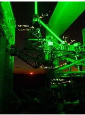
Fig. 5.Photograph of the left side of the telescope with the lasers in operation. The launch beam path from the exit to the first fold mirror is enclosed in a beam tube for safety and light scattering reasons. Between the first fold mirror and the mirror behind the adaptive secondary the beam is propagated in free air above the primary mirrors. From the mir-ror behind the secondary the laser bundle is launched to sky, forming the beacon constellation at a distance of 12 km.
beacons, there is a factor ∼10 margin built into the system to account for degrading laser power, optics, and atmospheric trans-mission, etc. The lasers are built into two boxes, one per side of the LBT. One of the boxes is shown in Fig.4. Inside each box we shape and direct the laser beams into the desired locations. Fol-lowing the beam train after the exit from the laser heads, we col-limate and pre-expand the beams to a 6 mm e12 diameter, rotate the polarization to match the Pockels cell gating units, steer the direction of each laser individually to position it on the constel-lation, send it to a common piezoelectric (PZT) mirror in the launch pupil plane, and let it exit from the box into the main beam expander. To make the set-up work, additional diagnostics and controls are built-in:
– Two cameras measuring the location of the beams in the field and pupil plane, feeding a loop to adjust the positions; – A specially developed white-light shearing interferometer to
control the beams collimation on demand;
– A power meter to measure the laser’s power and photo diodes to monitor the pulse shape and emission timing;
– A safety shutter to enable or disable the laser propagation to sky;
– The vibration compensating piezoelectric pupil mirror; – Several devices to control the temperature, humidity, and
cleanliness of the unit.
Being able to create a small spot at a distance of 12 km from the telescope requires a sufficiently large beam to be launched. The enlargement of the 6 mm laser beams and steering onto the axis of the telescopes are done by the launch telescope. A photo-graph of the launch path in operation is shown in Fig.5. It con-sists of a refractive aspheric beam expander and two large fold mirrors. The expander has been designed with ∼8 m focal length aspheric fused silica lenses, being held in the LBT’s steel frame as a mount. The expanded 40 cm aperture beam is reflected with
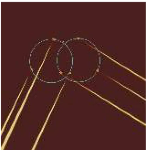
Fig. 6.Image of the double laser constellation on sky, taken with a small auxiliary telescope. Each bundle of lasers belongs to one side of the binocular telescope. The circles guide the eye, showing the constellation diameters of 4 arcmin on sky. The stars indicate the locations of the Rayleigh tip from where the scattered light is used for the wavefront sensing.
a fold mirror across the primary and with a second fold mir-ror behind the adaptive secondary towards sky. These two fold mirrors are manufactured from Borofloat (a borosilicate glass), using an internal lightweight honeycomb rib structure with an optically polished front plate. During the commissioning phase we found this structure to bend slightly due to temperature dif-ferences between the front and back plate, mainly driven by the small amount of laser light that is absorbed and therefore heats the surface. This effect made it necessary to implement a twofold correction mechanism: a counter heater on the back surface of this mirror to keep the temperature difference at a constant level, and an astigmatic compensation system in the beam. Consist-ing of two tilted flat glass plates this compensation unit can be adjusted remotely to minimize the spot sizes on the wave-front sensor together with focusing the beams. The lasers focus is adjusted by moving the small launch entrance lenses in the expander units along the optical axis.
Because the LBT is a binocular telescope with a large struc-ture, significant flexure and differences in pointing can occur between the mount and the mirrors. The laser and launch system are built into the centre piece of the steel structure and follow its movement. When setting up at the beginning of the night, or moving to a new object, the constellation (shown in Fig. 6) usually requires a new pointing correction. Finding the laser positions on sky is carried out with the help of the laser align-ment telescope (LAT) and a routine calculating the required movements of the large fold mirror, as described in detail by Sivitili (2016). Once located in the field of view of the patrol cameras of the wavefront sensor, the laser beacons are placed by a “click-and-go” procedure in the central aperture.
2.3. Sensing the laser beacons
On the downwards path the LGS light is collected by the two primary mirrors of the LBT and sent via the secondary and the tertiary mirror towards the science instruments. Figure7shows a drawing of the optical path and the multiple wavefront sensors units as installed at the telescope. After the telescope’s tertiary mirror, in front of the instrument rotator, a dichroic beam split-ter separates off the 532 nm laser light and sends it towards the
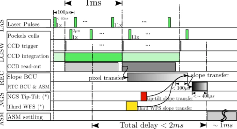
LGS wavefront sensor (LGSW). Light from the NGS passes the dichroic, is reflected by the LUCI entrance infrared-transmitting window, and is sent to the FLAO sensor. The infrared light passes the entrance window and enters the LUCI spectrographs. Both ARGOS LGS wavefront sensors are based on a Shack– Hartmann (SH) scheme to detect the LGSs. Details are described inBonaglia et al. (2014). Being located in a conjugated plane of the 12 km focus, a field stop with ∼400 diameter forms the entrance to the WFS optics. For each of the guide stars, a colli-mating lens re-images the pupil via a periscope onto the entrance of the Pockels cells. The periscope mirrors bring the beacon con-stellation closer together, and allow for field stabilization inside the sensor. The collimated beam – strictly collimated when the laser light comes from exactly 12 km – arrives at the Pockels cell assembly. This unit has been specially designed to ensure an excellent suppression over the large field of view of the Shack– Hartmann sub-apertures, 500 on sky or the corresponding 1.6◦ ray angle at the level of the Pockels cells. Due to the 8.4 m apertures of the primary mirrors, large ray angles are present at the Pockels cells assembly, prohibiting the use of standard commercial cells. The custom developed cells consist of dou-ble beta-barium borate (BBO) crystals in an optical arrangement ensuring the highest suppression over a large ray angle range. Applying a 9 kV rectangular voltage pulse to the crystals elec-trodes, the cells act as the optical shutter. In the range gating sequence the opening is applied ∼80 µs after the laser pulse has been sent to sky and then closed 2 µs later. All light that is scat-tered in the atmosphere before or after the high-voltage pulse is suppressed by a factor of more than ∼1000. This lets only those photons pass towards the CCD that have been scattered between 11.85 and 12.15 km above the telescope. At that sup-pression rate we have calculated the resulting wavefront error in each affected radial mode to be less than 8 nm RMS, sufficiently low to be of negligible influence. With the lasers repetition rate being set to 10 kHz, we accumulate the charge of ten pulses on the sensor before the readout is triggered. The complete timing sequence is shown in Fig.8. The readout of the CCD takes just less than 1 ms during which the analogue signals are transmit-ted to the ARGOS slope BCU. This unit digitizes the analogue pixel signals, performs the necessary calibration and computes the slopes. The operations are performed in parallel to the arrival of the pixel charges and thus ensures a minimum latency, being estimated to be <100 µs, with respect to the end of the readout. A particular feature of the ARGOS slope BCU is that it can asyn-chronously receive other WFS signals such as tip-tilt measure-ments from our APD or WFS slopes from the FLAO pyramid sensor. A final slope vector is concatenated and transmitted to the real-time computer (RTC) BCU that reconstructs and con-trols the adaptive secondary mirror (ASM). Without including the ASM settling time, the total latency in the timing sequence is less than 2 ms. Optically, after the gating units in the LGSW, each beam passes a focusing lens and a common collimator that forms three pupil images on a single lenslet array directly before the CCD. The optics are adjusted such that the three SH patterns are distributed over the CCD as shown in the upper left inset of Fig.7. Each sub-aperture spans 8 × 8 pixels, corresponding to ∼500× 500on sky, and is aligned such that the split frame transfer
does not cross the sub-apertures. More information on the wave-front sensor performance is given inBonaglia et al.(2014). The CCD itself is based on a deep-depletion technology, developed at the Max Planck semiconductor laboratory. It offers 264 × 264 pixels and 3.7 e−readout noise at a 1 kHz frame rate. Details can
Fig. 7.Optical path and CAD model of one of the wavefront sensors. The light from the LGSs enters from the right side in its 4 arcmin wide constellation. Patrol cameras enable a fast acquisition and position control of the guide stars. Inside the wavefront sensor units motorized mirrors stabilize the field and the pupil, driven by the signals from the WFS CCD. After that the gating units slice out the photon bunches originating from the 12 km distant scattering, letting a 300 m range (i.e. 2 µs) long part pass to the wavefront sensor detector. These Pockels cells units operate at the same 10 kHz as the laser pulses are sent to sky. The wavefront sensor detector accumulates the charge originating from 10 consecutive pulses, being read out at a 1 kHz frame rate. The wavefront sensor CCD frame of one telescope side with the three LGSs is shown on the left. Having passed a common microlens array in front of the detector, all three guide stars show a Shack–Hartmann spot pattern on the detector. From each spot the local wavefront slope can be measured, enabling the reconstruction and correction of the ground-layer turbulence. Because LGS spots are often larger than NGSs, the sub-aperture’s field of view amounts to ∼500
sampled with 8 × 8 pixels on the CCD frame.
2.4. Correcting the ground layer
The core of the adaptive optics computation with ARGOS is car-ried out by the wavefront sensor computer, as sketched in Fig.9. It receives the PnCCD analogue signals, and finally transmits a slope vector to the LBTs adaptive secondary mirrors (ASM) where the wavefront reconstruction is performed. This compu-tation architecture has to carry out several main tasks and fulfil tight constraints:
– Digitizing the analogue signal from the ARGOS LGS wave-front sensor camera;
– Calibrating and background subtracting the frames;
– Computing the x and y local wavefront gradients for three SH pupils, each containing about 176 sub-apertures, hence 1056 displacements;
– Providing the interfaces to the other wavefront measure-ments, in particular to the NGS tip-tilt, mandatory for the AO operation, but also for the measurements of a third WFS providing an NGS or sodium guide star measurement. This allows a “hybrid” AO operation;
– Calculating the global tip and tilt signals for each LGS and controlling the overall field position correction on the CCD; – Delivering a global tip-tilt signal to drive the uplink
correc-tion performed by the pupil mirror in the launch system; – Transmitting the wavefront measurements to the LBT
real-time reconstructor and deformable mirror controller. ARGOS has three different wavefront sensing measure-ments: the three combined laser measurements, the NGS tip and tilt, and a third wavefront sensor, that can be used to perform a “hybrid” correction scheme, combining GLAO with a SCAO mode. Currently the FLAO pyramid sensor can be concatenated into the slope vector. Those measurements are collected in a vector sf = [s3LGS; sTT; sFLAO], for a total of 1600 slope
mea-surements, and are sent to the ASM. At the ASM a
reconstruc-tor converts the slopes into the mirror Karhunen–Loève (KL) modal basis, using an integrator control. Once computed, the modes are then projected on the command space of the ASM by matrix multiplication, which is then directly used by the inter-nal control of the ASM. An additiointer-nal disturbance vector can be added to this command vector, which is typically used for calibration.
The main element to be calibrated from the ARGOS point of view is the reconstruction matrix used to perform the mapping, from the several wavefront measurements to the modal ampli-tudes. This matrix is obtained by pseudo-inversion of the inter-action matrix, which is part of the calibration of the ARGOS AO loop and is obtained as follows: utilizing a push-pull sequence, modes are successively applied to the ASM (i.e. by using the disturbance vector mentioned above). For each of them the wavefront measurements are recorded, thus constructing the matrix IM of dimension (Nslopes × Nmodes). The amplitudes of the push-pull of each mode is optimized to provide a uni-form signal-to-noise ratio by re-scaling the applied amplitudes to have the same slope standard deviations (for more details see Esposito et al. 2010). An example of the full interaction matrix is shown in Fig.10. The final ARGOS reconstructor is a block-wise matrix containing the GLAO reconstructor R3LGSsand RTT
or RFLAOdepending on which sensor is used for the tip-tilt
cor-rection. Considering the symmetry of the LGS constellation, the GLAO reconstructor that estimates the ground layer and aver-ages out higher-layer altitudes is obtained by taking the pseudo-inverse of the three LGS interaction matrices at once: R3LGSs =
I M3LGSs† , where I M3LGS is of dimension nslopes× nmodes or
typ-ically 1057 × 150. The block-wise reconstructor provides great flexibility regarding which wavefront sensor is used. In addition to these wavefront measurements and the modal reconstruction, ARGOS uses the NGS wavefront sensing unit (FLAO) to mea-sure slowly changing non-common path aberrations between the
... ...
... ...
... ...
Fig. 8.Sketch of the complete ARGOS timing sequence from laser pulse launch down to the settling of the adaptive secondary mirror (ASM). The 40 ns laser pulses are generated at a 10 kHz rate. The back and forth propagation in the atmosphere takes 80 µs at which point the Pockels cells are opened for 2 µs (corresponding to a 300 m slab), thus exposing the PnCCD to the laser photons. Ten successive pulses are integrated on the detector, the readout is triggered taking just less than 1ms. The analogue outputs are directly sent to the slope BCU unit, which digitizes the analogue pixel signals and perform all the necessary operation to compute the Shack–Hartmann slopes in a parallel manner, thus minimizing the delay (est. <100 µs) after the end of the CCD read-out. Asynchronous signals (indicated by a ?), a particular feature of ARGOS, such as tip-tilt signals from our APD or the FLAO pyramid slopes, can be concatenated to the LGS signals. The final slope vector is transmitted to the real-time computation BCU for reconstruction and control of the ASM. Disregarding the ASM settling time, the total delay is less than 2 ms.
ARGOS Slope Vector WFSCamera
Pyr WFS Slopes
WFS Camera Frame (Input) TT Slopes (Input) FLAO Slopes (Input) ARGOS Slopes (Output) APD Unit Slopes
ASM Switch BCU ASM BCU Diagnostic broadcaster Diagnostic to Workstation Real Time Diagnostic Only if used as TipTilt sensor
ARGOS Reconstruction Matrix With APD for modes 0,1 and LGSW for modes 2 … 150 Mo des 0 1 2 . . . 15 0
ARGOS Reconstruction Matrix
With PyrWFS for modes 0,1 and LGSW for modes 2 … 150
Analog signals
Fig. 9.Sketch of the ARGOS WFS computer and reconstruction matrix. First, the computer receives the analogue signals through 8 channels from the ARGOS pnCCD camera. It digitizes the data and sends the pixel values to the computing part of the board for LGS slope com-putation. In parallel, the computer can also receive the NGS tip-tilt slopes and the slopes from a third WFS, currently from the first light AO (FLAO). Finally, a slope vector is assembled and sent to the ASM switch BCU, selecting the working wavefront sensor, and then for-warded to the ASM control.
LGS optical beam and the light on the pyramid sensor. This “truth” sensing is projected back to the LGS slopes and is added as new offsets in the ARGOS wavefront sensing computer.
Fig. 10.Image of the ARGOS interaction matrix showing the x- and y-direction slopes for each KL mode. Since the WFSs are SH, the image of the interaction matrix is the derivative of the wavefront in the x and y directions. The bottom line in the matrix displays the low-order modes: (from left to right) Tip, Tilt, Astigmatisms, Focus, and Coma. The inset shows 18 modes for illustration. Values are in arbitrary units, scaled from −1 to 1, while the interaction matrix used for the computation is in units of RMS wavefront deviation divided by unity slope [m arcsec−1].
2.5. Operating ARGOS on sky
Getting the adaptive optics loop closed and operational on sky requires the whole chain of system items to be functional: from the telescope collimation itself to the focusing and shaping of the laser beams on sky, acquisition of the laser beams on the wavefront sensor, locking the LGS guiding loop, and the acqui-sition of the natural tilt star, and finally to a sequence of actions to close the adaptive optics loop. Having the loops closed then enables the science integrations to start. In the following, we briefly describe the acquisition and loop operations, and we pro-vide insights into the way the laser star and tilt guide star oper-ation is handled upon offsetting, sky frames pointing, and asyn-chronous interruptions such as aircraft passage or satellite clo-sures. More details on the adaptive optics operation are given in Busoni et al.(2015)
2.5.1. Acquiring the stars
Pre-acquisition. After the telescope is properly collimated, a pre-set is executed to slew to the science field where the Satellite Avoidance System allows the laser operator to enable the prop-agation of the six lasers (see e.g.Rahmer et al. 2014). To simul-taneously align the LGS constellation on both of the telescope’s optical axes, the laser alignment telescope (LAT) is used. This allows the three LGSs to be acquired in the 4000field of view of the patrol cameras of each LGSW.
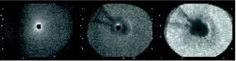
Fig. 11.One of the LGSs as seen on the patrol camera. This camera has a field of view of 1 arcmin and is used to acquire the lasers in a click-and-go procedure. Left panel: clear sky view of the laser as seen by this un-gated camera, focused to 12 km. The laser spot vanishes in the central hole, being the entrance aperture of the WFS. In the mid-dle panel scatter from lower altitude cirrus clouds can be seen, clearly distinguished from the LGS. Right panel: thick clouds make the star at 12 km vanish completely.
Beam sharpening. The laser launch optics are equipped with two active devices to compensate for focus and astigmatism aberrations in the uplink path. While the need for focus com-pensation is obvious, astigmatism is introduced by the thermal bending of the launch mirrors LM1 and LM2 (see Fig.5) in the launch system itself. To restore the laser beam quality the com-pensator position must be optimized by running an automatic procedure that scans the entire range of the focus stage while recording images of the laser spots on the LGSW patrol cameras in an intra-focus/extra-focus scheme. For each focus stage posi-tion the spot size is measured along two orthogonal direcposi-tions. The distance between the two minima in the spot length curves is proportional to the total amount of astigmatism in the uplink propagation. The value is converted to a compensator adjustment by using a model of the launch optics.
Final-acquisition. The LGS acquisition requires human inter-vention: the ARGOS operator has to look at the LGSW patrol camera display and to click on the position of the LGS spots that are easily identifiable by eye. This has been shown to be much more robust than an automatic procedure, especially in the case of thin clouds creating scattered images on the LGSW patrol cameras. Images of the LGS on one patrol camera are shown in Fig.11. As soon as the operator confirms the LGS acquisition, the LGS guiding loop is automatically closed. This algorithm uses the mean tip-tilt slopes recorded by the three SH sensors to evaluate the common drift of the LGS constellation on sky and to apply a proper tip-tilt correction to the launch system pupil mirror. This process is a real-time loop, running at 1 kHz imple-mented in the ARGOS slope BCU. The offset accumulated by the laser system pupil mirror is periodically offloaded to the LM1 that has the same optical effect on sky but with a larger stroke.
Together with the guiding loop the vibration compensation system is activated. This system uses the piezoelectric launch system pupil mirror compensating for the uplink laser jitter. The system relies on the measurement of eight accelerometers attached to the back of the 2 LMs in the launch optics and it implements an open-loop feed forward control and a Kalman recursive filter. (Details inPeter et al. 2012).
In parallel with the process of LGS acquisition, the NGS sensor is configured and the natural star chosen by the LUCI script as the tip-tilt and truth sensing star is acquired. As ARGOS makes use of the FLAO hardware to implement the NGS WFS, it also uses its control procedures to move the acquisition stages on target, to configure the WFS hardware, and to activate the real-time communication with the slope computer.
2.5.2. Enabling the adaptive correction
Having both LGS and NGS acquired on the respective WFS automatically triggers the closure of the GLAO loop. This con-sists of several operations performed in sequence:
(1) Configure the real-time computer (RTC). The reconstruc-tor matrix is selected according to the chosen configuration (APD vs Pyramid, binning of pyramid WFS) and to the mag-nitude of the NGS. The reconstructor matrix is uploaded to the ASM RTC. The ARGOS slope computer BCU is re-configured, if needed.
(2) Close the tip-tilt loop. The real-time communication between the slope computer and the reconstructor on the ASM is enabled, with all modal gains set to zero. Then tip-tilt gains are ramped up from 0.01 to 0.2 in a few seconds.
(3) Offload focus to time-of-flight. The altitude to which the LGSW is conjugated can be varied by modifying the time-of-flight, i.e. the time passing between the trigger of the laser pulse and the signal that opens the gating units in the LGSW. This interval, being nominally 80 µs and corresponding to the round-trip of the laser pulses to 12 km, is adjusted to null the focus term measured by the SH WFS. This ensures a smooth operation when the LGS loop is closed.
(4) Close the LGS loop. The gain of the modes controlled by the LGS are increased in steps from 0.001 to 0.1 in a few seconds.
(5) Start the Truth Sensing. The FLAO control software com-putes autonomously the true wavefront error by projecting on the same modal basis that is used in ARGOS for the adaptive correction. The modal coefficients are read by the ARGOS control software and converted into LGSW signals through a multiplication by the LGS interaction matrix. This signal vector is integrated to the current LGSW slope-offset vector for all modes but the focus. Focus is offloaded to the time-of-flight, as described above, to retain the maximum dynamical range of the SH sensor.
(6) Optimize modal gains. As a last step, the modal gains can be optimized. An optimization script that scans a range of modal gains and searches for the values that minimize the WFS signal variance can be optionally executed. The oper-ator has the option to adjust the values of the modal gains (grouped in three sets: tip-tilt, modes from 2 to 36, and higher modes) from the ARGOS control GUI. This procedure is not always required for the modes controlled by the LGSW because the sensitivity of the SH sensor is stable under most operating conditions. However, it is always required for tip and tilt modes because the quad-cell sensor and the pyramid WFS sensitivity depends on PSF size, which in turn depends on seeing.
2.5.3. Dithering, offsets, and asynchronous interruptions During the execution of a LUCI-ARGOS observing block, there are several circumstances that require pausing the adaptive optics correction for a short period. These include offsetting the field or stopping the laser propagation due to satellite or airplane transit. In the first case, because of the way the LBT handles binocular offsets between the mount and the two telescopes, it is difficult to predict whether the LGS light will stay on target. The easiest solution is to pause the LGS loop by setting the mid- and high-order modal gains to zero. The size of the offset then plays a role in the way the LGS loop is resumed:
– Small offsets, within the reach of the FLAO field positioning stages (30× 20), the NGS loop is paused, the board stages
are then moved to re-centre the star on the tip-tilt sensor and both the NGS and LGS loops are resumed by ramping up in two steps the modal gains to the original value. During the offset execution, the truth sensing is disabled.
– Larger offsets, where the NGS cannot be re-acquired because it is out of the field reachable by the FLAO stages, the whole adaptive optics loop will simply remain paused. When point-ing the telescope mount back after the large offset, the adap-tive optics loop will be automatically resumed, with the same procedure as for small offsets.
When a satellite or an airplane transit requires laser propaga-tion to be stopped, the control software automatically pauses the LGS loop and then stops the lasers: this permits the closed-loop observation to quickly resume as soon as the lasers are propa-gated again on sky without the overhead of a new acquisition. The control software tries to resume the loop automatically. If it fails, it leaves to the ARGOS operator the task of reacquiring the LGSs, which may have drifted out of the field during the pause. In the current telescope control software scheme there is no way for ARGOS to interact with the LUCI script sequencer, leav-ing it unaware of these kinds of events and unable to react and optimize the observation. Instead the AO loop status is recorded in the fits header. Since most interruptions are short, the LUCI integration just can continue, with a minor reduction in the data quality.
2.6. Spectroscopy with ARGOS
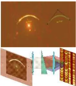
One of the really unique capabilities that ARGOS offers is the combination of the GLAO with NIR spectroscopy. To our knowl-edge LUCI-ARGOS is currently the only facility in the world that can deliver spectra of multiple objects with 0.2–0.300 spa-tial resolution and spectral resolution R ∼ 10 000 at the same time. Additionally the 4 × 4 arcmin masks for LUCI can be cut to custom shapes matching the object under study, or can contain up to ∼70 slits (depending on length) to be placed on individual objects for a high multiplexing advantage. In Fig. 12a sketch of such a custom slit observation is shown. Using HST or an ARGOS pre-imaging campaign, we design a mask that matches a lensed arc, and a second identical slit to allow nodding between the two. Additionally, a slit of the same width is always placed on one or more reference stars in the field and its nod position to control alignment during the observation and to have a spa-tial and spectral reference upon data reduction. Adding align-ment boxes on objects over the field finalizes the design step. This design file is sent to the observatory for the laser cutting and cryogenic insertion of the masks for the upcoming semester. Upon observation the mask is grabbed by the robot inside LUCI and inserted in the instrument’s focal plane. The ARGOS obser-vation then approximately follows the scheme for seeing-limited MOS observations with some specific additions:
– in the observation preparation, and already in the design of the mask, the location of the tilt star needs to be taken into account. All planned dither points must lie within the capture range of the FLAO board;
– during pointing of the telescope the set-up follows a two-stage process: the telescope first needs to set its active optics on a suitable bright star, not too far from the object, and then the telescope and FLAO board position are set to catch the tilt star on the pyramid. This process is handled by the tele-scope control and does not need the attention of the observer.
Fig. 12.Basic principle of curved slit spectroscopic observations with ARGOS plus LUCI. Top panel: Ks-band image of a gravitationally
lensed object (the 8 o’clock arc) with the mask design overlaid. From the design, a custom, laser cut mask is made and inserted and stored cryogenically in the LUCI instruments. During the observation only the light from the desired object enters the spectrometer. The ARGOS sys-tem allows tiny slits to be used with all light from the object passing through. As a result the spectral resolution is high and the skylines are well resolved. This allows for much better object flux extraction.
In parallel the LGSs are launched and the LGS acquisition process is executed, as laid out in Sect.2.5.
– Once the AO loop is closed, the telescope pointing can be aligned to the MOS mask in the LUCI focal plane. With the ARGOS slits usually being of the order of 0.300 wide,
this process needs special attention since small misalign-ments quickly result in light lost at the slits. Therefore, we have developed our own routine that measures and aligns the required offset and rotation on the through slit image and ref-erence objects, preferably some background galaxies, chosen during the mask design.
3. GLAO performance on sky
From 2015 to 2017, ARGOS has spent approximately 100 nights and many days of commissioning. With multiple systems only being available on site, we had to bring the subsystems together and make them work at the telescope. While usually an extended period in the laboratory as a complete system would be desir-able, the pure size of such a test facility and the complexity of the ASM usage did not allow for laboratory system test-ing. Having seen continuous progress, now the full system in binocular mode is finally available for the community. Commis-sioning and AO results can be found in several conference pro-ceedings (Busoni et al. 2015;Orban de Xivry et al. 2015,2016; Rabien et al. 2017). Now, we do see a system that is capa-ble of conducting science operation feeding the two sides of LBT simultaneously with LGS corrected light. The capability of doing full binocular operation with ARGOS and two LUCIs is a real boost for the science outcome. Having two 8.4 m tele-scopes available at the same time with a GLAO corrected PSF of 0.200–0.300 in size will help some science cases to proceed. Since the PSF size compares well with HST data, ARGOS can complement imaging taken with HST with K-band observations at similar resolution. In the following sections, we discuss the
Fig. 13.Left panel: histogram of the mag(R) of the NGS used in 100 science fields during 2016 and 2017 commissioning runs. The val-ues represent the star magnitude taken from the NOMAD Catalog, as used to produce observing script. Right panel: distribution of the GLAO performance as a function of the NGS magnitude. The GLAO gain has been evaluated by the ratio between the full width half maxi-mum (FWHM) measured in open-loop and closed-loop LUCI/ARGOS images. No clear trend is visible in the plot, suggesting a limited impact of the NGS brightness on the GLAO peformance.
performance of ARGOS based on several metrics. First, we look at the adaptive optics performance, i.e. the wavefront error RMS, and show that it matches our theoretical expectations. Then, in Sect.3.2we analyse the uniformity of the correction over the full 4 × 4 arcmin field of view and conclude that we have marginal observational effects, irrespective of the tip-tilt guide star loca-tion in the field. In Sect. 3.3we look at the performance over an observing period showing that GLAO with ARGOS is also a full width at half maximum (FWHM) stabilizer over time, producing a more consistent FWHM than seeing-limited obser-vations. In Sect. 3.4, we summarize the GLAO performance, i.e. the improvement in FWHM with ARGOS with respect to seeing-limited mode, over our commissioning period. Finally, in Sect. 3.5, we discuss the GLAO corrected PSF which is well matched by a Moffat analytical profile as expected from the-ory. One limitation of our performance analyses is the lack of a dedicated turbulence profiler which would provide the strength of the turbulence as a function of altitude while operating with ARGOS. This is further discussed at the end of Sect.3.4. 3.1. Adaptive optics performance
A critical parameter of an AO system based on LGS tomography is the availability of a suitable NGS within a few arcmins of the science field. A statistical analysis of the more than 200 science fields observed during the last 2 years of commissioning shows that 40% of the time the system worked with an NGS fainter than 14th magnitude, as shown in Fig.13and that a few targets were observed with NGS of about 17th magnitude.
As detailed in Sect.2.4, the ARGOS LGS wavefront sen-sor runs at a fixed framerate of 1 kHz, while the NGS wavefront sensor framerate can vary between 100 Hz and 1 kHz depending on the star magnitude. At the faint end, the typical tip-tilt resid-ual measured by the NGS WFS amounts to 150 nm rms. How-ever, the pyramid WFS sensitivity strongly depends on the size of the NGS PSF so the tip-tilt residual measured on sky is under-estimated. The ratio of the optimal gain applied to the tip-tilt modes on sky (e.g. 2.5) to the value used in daytime operation when a diffraction-limited light source and 1 kHz frame rate are used (e.g. 0.75) gives a conversion factor to properly scale the on-sky tip-tilt residual. Considering a faint NGS the residual jit-ter amounts to ∼50 mas, so about 1/4 of the closed-loop PSF FWHM obtainable in GLAO assisted images. In conclusion, the
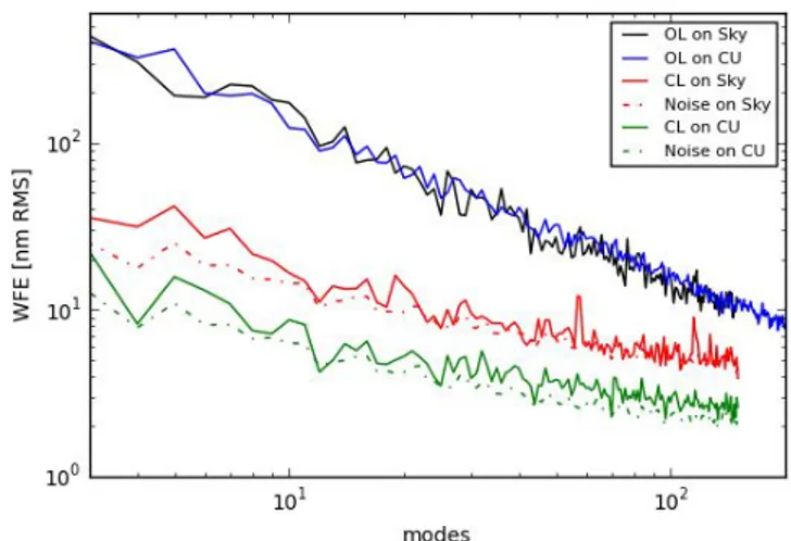
Fig. 14.Modal decomposition of the wavefront measured by the LGS WFS. The tip-tilt modes have been removed because they are sensed by the NGS WFS. In open loop (OL) the integral of the measured WF amounts to 860 nm rms in daytime, using the prime focus calibration unit (CU) (blue line), and to 830 nm rms on sky (black line). When the AO loop is closed the WFE are lowered to 55 nm rms (green) and 120 nm rms (red) respectively. The dashed lines show the modal decom-position of the covariance matrix for the SH WFS measurement error evaluated considering the daytime (green) and on-sky (red) parameters of seeing, flux, and spot dimension.
NGS brightness has a very limited impact on the GLAO perfor-mance (see Fig.13, right panel).
Evaluating the performance on sky of the LGS wavefront sensors is difficult because the quality of the tomographic mea-surement is strongly affected by the vertical distribution of the atmospheric turbulence and because the LGS WFS are only sen-sitive to the lower layers of the atmosphere. A possible approach is to compare the performance of the LGS WFS on sky with that obtained in daytime, using the prime focus calibration units and emulating the atmospheric turbulence through the adaptive sec-ondaries.
In daytime the system operates under well-known condi-tions: the injected disturbance is equivalent to a 0.800 seeing (r0= 0.125 m) with a Kolmogorov spectrum represented by 672
Karhunen–Loeve modes, the daytime LGS flux can be tuned to reproduce the same S/N as obtained on sky (∼30, equivalent to a flux of 650 e−/subap/ms) and the LGS spots from the
calibra-tion source have a FWHM of ∼0.900 with no elongation. The turbulence is only applied to a layer conjugated to the ground where the three LGS WFS measure up to 150 modes. Neglect-ing the tip-tilt terms, the typical WFE measured on the higher order modes by the LGS WFS amounts to 860 nm rms, as shown by the blue line in Fig.14. Closing the AO loop the residual WFE lowers to 55 nm rms, as given by the green line in the figure. This value can be compared with the covariance matrix CNobtained
by multiplying the noise propagation coefficients by the Shack-Hartman measurement error reported inCubalchini(1979),
CN= (ITMIM)−1σ2m, (1)
where IMis the LGS WFS interaction matrix and the
measure-ment error σ2mcan be retrieved fromHardy(1998),
σm= π2 4SNR 3d 2r0 !2 + θdλ !2 1/2 [rad] , (2)
where d = 0.55 m is the sub-aperture dimension projected on the primary mirror, θ the LGS spot dimension and λ= 532 nm.
Fig. 15. Colour composite image of NGC 2419 from J, H, and Ks
images. On the left side the full 4 × 4 arcmin field of LUCI is shown, fitting well the whole cluster. To the right a zoom into the cluster core, showing the richness and density. Taken during the commissioning of ARGOS, we can use this example to measure the adaptive optics perfor-mance over the field. NGC 2419 with its large number of stars provides a good map for the uniformity of the FWHM.
Considering the daytime operating conditions described above, the modal decomposition of the LGS WFS measurement error is shown by the dashed green line in Fig.14. Digging into data col-lected on sky it has been possible to find similar input conditions, where the LGS WFS were measuring an open-loop WFE of about 830 nm rms (black line) and a residual of 120 nm rms (red line). However, the LGS spots on sky typically have a FWHM of θ ∼ 200, increasing the LGS WFS measurement error by a factor
of 2.2. Taking into account the increased spot size and the on-sky parameters, the residual WFE measured by the LGS WFS is in agreement with the modal decomposition of the covariance matrix, as can be seen from the red dashed line.
3.2. Imaging performance over the field
Figure15shows the image of NGC 2419, an old cluster of stars in the halo of the Milky Way. The cluster has been visited during the ARGOS commissioning several times. Apart from the sci-entific insight into the galactic potential and the cluster colour magnitude diagram (CMD) outlined in Sect.4.1, the cluster also provides us with nicely distributed stars as PSF probes for the adaptive optics performance. Judging the correction quality in single-conjugate adaptive optics is usually done by measuring the Strehl ratio, comparing the PSF to the diffraction limit. In GLAO the correction rarely reaches the diffraction limit, with the main focus being on the uniformity and wide-field performance. In analysing the resulting images we selected the FWHM as a reasonable metric for the PSF.
With the large LUCI field available we can probe the PSF properties over the 4 × 4 arcmin fields. Figure 16 shows the performance over the field as obtained in an observation of NGC 2419 over the J, H, and Ksbands. In this observation under
seeing conditions of ∼100, as measured on the differential image
motion monitor (DIMM), the measured PSF size in J, H, and Ks
amounts to 0.2700± 0.04, 0.2500± 0.04, and 0.2500± 0.04,
respec-tively, in the inner 1 arcmin radius. Towards the outer areas an increase of ∼0.0200in all bands can be seen.
Another inherent property of the GLAO system is the lack of dependence of the PSF shape on the tilt star location. Within the ARGOS and FLAO set-up we are able to chose the location of the tilt star within a 2 × 3 arcmin field, asymmetric in the LUCI fields, as given by the travel range of the FLAO stage assembly.
Fig. 16.Analysing the FWHM over the field of the NGC 2419 data shows the ARGOS performance over the full LUCI2 field of view, mea-sured in 100
seeing. In the upper panel are indicated the positions of all the stars used to measure the azimuthal FWHM variation in the field. Colours separate stars at less then 1 arcmin (blue) and 2 arcmin (red) radial distance from the field centre. The grey encircled asterisk marks the location of the NGS at 225◦
, that has been used to track the tilt and low-order modes. A small (<15%) radial increase from 0.2500
to 0.2800
of the FWHM from the centre to the detector edge is possibly seen in this data set. There is one panel shown for each of the J, H, and Ks
Fig. 17.Temporal evolution of an imaging observation of the XID2028 source. The natural seeing in the visible from the DIMM measurements is shown as a green line and varies between 0.800
and 1.000
over this ∼2 h observation. The individual points are the measured FWHM from fitting a Gaussian to a resulting 1min integration of six stacked frames. The red stars indicate the FWHM measured in the LUCI1 frames, the blue diamonds that in LUCI2. With this observation of an extragalactic source, no sky frames are taken, and no open-loop data is available. The one red star at 0.500
is a frame marked with “paused”, indicating a laser propagation stop upon aircraft passage while still being closed on the tip-tilt star. The median performance on the LUCI frames over this full 2 h operation amounts to 0.2600
with LUCI1, and 0.2500
with LUCI2.
Within many observations we have not seen a detectable dependence on the tilt star location in the field. For the many science cases that suffer from sparsely available suitable NGSs, this will be of major importance.
3.3. Imaging performance over time
Many science cases require a stable and well-defined PSF over the observing period. With the natural seeing being often highly variable, the combination of many images over the observation period results either in the combined image being affected badly by the increased seeing moments, or a selection of frames may be required. Getting rid of the ground-layer turbulence contribu-tion does help in that respect. We have seen long exposure peri-ods where the seeing measured on the DIMM had high varia-tions, while in the corrected images a fairly constant PSF size has been achieved. Of course, if the variation takes place in the high layer, the GLAO PSF will follow the seeing variation. In Fig. 17the PSF FWHM of an imaging observation under fairly con-stant conditions is shown. The object of interest in this observa-tion is XID2028 located at z = 1.5930, originally discovered in the XMM-COSMOS survey, a star forming QSO, being thought to be in the “feedback phase”. The LUCI observations here com-plement ALMA data on the same object, resolving extended dust emission in the Ks band coincident with a point source at 0.100
resolution detected by HST. We observed this object for ∼2 h in binocular mode with both LUCIs in Ksband. With the individual
integration times being 10 s long, each data point is already a stack of six images taken in integrated mode. During this 2 h period the median FWHM on the two LUCIs is 0.2600and 0.2500with a
stan-dard deviation of 0.01400and 0.0200, respectively. The data taken in this observation has been published inBrusa et al.(2018).
Fig. 18.ARGOS commissioning performance plot, summarizing many imaging observations done during commissioning. Taking the open-loop FWHM points as seen in sky frames of an observation and over-plotting the achieved GLAO FWHM, we can judge the “improvement” in FWHM. The plot shows 123 data points taken from 43 observations over the J, H, and K bands (green, blue, and red points, respectively). Lines mark the “factor 2” and “factor 3” improvement, and the yellow diagonal of “no correction”. The “N3.75 camera limit” marks the small-est possible size measurement with the specific camera in use, possess-ing a 0.11800
pixel scale.
3.4. GLAO performance
From early 2015, when the first successful loop closures could be carried out, until late 2017, the technical commissioning was always accompanied by an attempt to get data on sky in parallel. This strategy proved to be quite helpful as issues in the whole chain of units–from telescope to FLAO, ASMs, ARGOS, and finally LUCI as the receiver of the infrared photons–could be found and improved. In the case of nearby galaxies or galactic objects, sky frames are usually required for background subtrac-tion. Moving to sky with ARGOS is usually done by opening the high-order and the tilt loops since the sky pointing may be out of the acceptance cone for satellite avoidance (see Sect.2.5.3). For performance measurements this offers an opportunity to measure the open-loop PSF size and compare it to the closed-loop perfor-mance. Having seen a variety of weather and seeing conditions over the commissioning nights, we can now draw a plot for the open- versus closed-loop PSF size giving the GLAO improve-ment metric. Figure18shows the collection of data points out of 43 observations delivering 123 data points in the J, H, and K bands for this analysis. Observation attempts in very poor con-ditions, high seeing, or winds with the AO loop crashing have been excluded from this plot since under routine observing pro-grammes one would expect to switch to a different programme.
In summary the GLAO system can deliver an improve-ment of a factor of 1.5–3. The K-band average improveimprove-ment from these data points is 2.14, with a 0.2600 median PSF size. Nevertheless, this value gives an average over a technically improving system under commissioning conditions. A future routine usage of ARGOS will yield a picture that is statistically more solid. Since LBT had no turbulence profiler in operation over the commissioning period, we could not study the influ-ence of uncorrected high-altitude turbulinflu-ence layers within this data set. For this reason we started a SLODAR implementation (Mazzoni et al. 2016), and built a MASS unit (Kohlmann 2018) that may be installed in the future as facility devices, helping to decide whether a GLAO observation will yield high gain.
−0.5 0.0 0.5 [arcsec] −0.5 0.0 0.5 data [adu]3500 3550 3600 3650 3700 3750 3800 −0.5 0.0 0.5 [arcsec] −0.5 0.0 0.5 fit [adu]3500 3550 3600 3650 3700 3750 3800 −0.5 0.0 0.5 [arcsec] −0.5 0.0 0.5 residual [adu]−20 −10 0 10 20
Fig. 19.Illustration of the GLAO corrected PSF based on a combined K-band image of a total of 3.8 min exposure time. Left: Point source in the field. Middle and right: Fit by a Moffat profile and its residual after subtracting the model from the data, respectively.
3.5. Shape of the GLAO corrected PSF
It is well known that the PSF produced by a GLAO system does not exhibit diffraction-limited features, but is qualitatively very similar to a seeing-limited PSF (see e.g. Andersen et al. 2006). This means the GLAO PSF is well fitted by a Moffat function
I(r)= I0[1+ (r/R)2]−β (3)
with R the core width related to the FWHM by FW H M = 2R
√
21/β− 1, and β the power index of the function, with smaller
index leading to larger wings. The seeing-limited PSF under Kolmogorov turbulence is well modelled by β ≈ 4.77, but real PSFs typically have larger wings or equivalently smaller β due to imperfection in the optics (Trujillo et al. 2001). The GLAO PSFs are similar and have a power index between 2.5 and 4.5 (Andersen et al. 2006).
As an illustration of the delivered ARGOS PSF, we analysed J-, H-, and Ks-band images from a typical good and stable night.
The data fit and residual of a single PSF is shown in Fig.19. In total we fit several hundreds of elliptical Moffat functions to single and combined frames and obtained the following results: (1) For the J-band, we have β= 3.4±1.3 and FWHM = 0.3400±
0.04;
(2) For the H-band, we have β= 3.2±0.9 and FWHM = 0.2800± 0.03;
(3) For the Ks-band, we have β = 2.5 ± 0.6 and FWHM =
0.2100± 0.02.
We see that β and the FWHM becomes smaller at longer wavelengths which reflects the fact that the PSF is better cor-rected with a more pronounced core (corcor-rected) and wings (uncorrected). These values also fall in the predicted range obtained by GLAO simulations. Flux residual amounts to less than 1% and are typically around 0.2%, which again match the expectation inAndersen et al.(2006).
4. Selected science observations with ARGOS
Many science cases can profit from a GLAO reduced PSF size. From the many objects visited during the ARGOS commission-ing which were used as part of the performance testcommission-ing and science verification, we showcase the use of ARGOS with few selected science cases in this section. Ordered from near to far, we show the following observations:
– NGC 2419, a distant Galactic globular cluster. The enhanced resolution allows us to overcome crowding effects and mea-sure precise CMD and identify variable stars;
– NGC 6384, where the enhanced resolution of ARGOS extends nuclear and star cluster science to a distance of 20 Mpc; 14 15 16 17 18 19 20 21 22 -0.2 0 0.2 0.4 0.6 0.8 1 J0 [mag] (J-Ks)0 [mag] 14 15 16 17 18 19 20 21 22 -0.2 0 0.2 0.4 0.6 0.8 1 J0 [mag] (J-Ks)0 [mag] 14 15 16 17 18 19 20 21 22 -0.2 0 0.2 0.4 0.6 0.8 1 J0 [mag] (J-Ks)0 [mag] α/Fe=+0.2 α/Fe=+0.4 14 15 16 17 18 19 20 21 22 -0.2 0 0.2 0.4 0.6 0.8 1 J0 [mag] (J-Ks)0 [mag]
12Gyr, -2.2dex, α/Fe=0.0
14 15 16 17 18 19 20 21 22 -0.2 0 0.2 0.4 0.6 0.8 1 J0 [mag] (J-Ks)0 [mag] 0 50 100 150 200 250 300 350 400 450 0 20 40 60 80 100 120 140 160 180 Number of stars
Projected distance from NGC2419 center [arcsec] 0 50 100 150 200 250 300 350 400 450 500 14 15 16 17 18 19 20 21 22 Number of stars KS [mag] ARGOS (7118 # stars) Seeing (4764 # stars)
Fig. 20.Upper panel: NGC 2419 colour magnitude diagram from data taken during commissioning nights 2016 Oct 19, 23, 24, and 26. The magnitudes are corrected for foreground extinction as indicated by the magnitude subscript. Shown are sources with S /NJ,Ks > 10 (blue
cir-cles), all detections (small grey dots), and the known RR Lyrae (and other) variable stars in NGC 2419 (large solid red dots). For reference, we show with a solid red curve an isochrone adopting the literature val-ues for its age and metallicity and [α/Fe]= 0.0 dex. Magenta and blue curves in the background show a comparison to enhanced [α/Fe]= 0.2 and 0.4 dex isochrones (see Sect.4.1). Middle and lower panels: number counts of stars as a function of magnitude and as a function of distance to the cluster centre. The green histogram shows the ARGOS number counts, while the red line shows the detected stars in non-GLAO data. (Details in Sect.4.1)
– PLCK G165.7, a massive lensing cluster, where LUCI-ARGOS K-band data complements HST imaging, contribut-ing to lensed image family identification;
– Spectroscopic measurements of high-z gravitationally lensed galaxies. Utilizing the custom slit capabilities, we match the shape to the curved arcs and with ARGOS delivering a small PSF size we can probe the objects at high spectral and spatial resolution.