ALMA MATER STUDIORUM
UNIVERSIT `
A DEGLI STUDI DI BOLOGNA
Dottorato di Ricerca in Ingegneria Biomedica, Elettrica e dei
Sistemi
Dipartimento di Ingegneria dell’Energia Elettrica e
dell’Informazione “Guglielmo Marconi”
Ciclo XXX
Settore concorsuale: 01 - A6 Ricerca Operativa Settore scientifico disciplinare: MAT/09 Ricerca Operativa
MODELS AND ALGORITHMS FOR
OPERATIONS MANAGEMENT
APPLICATIONS
Presentata da:
ANDREA BESSI
Coordinatore Dottorato:
Chiar.mo Prof. Ing.
DANIELE VIGO
Supervisore:
Chiar.mo Prof. Ing.
DANIELE VIGO
INDEX TERMS
Derivative Free Optimization
Black Box Optimization
Computer Vision Algorithm
Sequential Approximate Optimization
Parameter Tuning
Contents
Abstract vii 1 Introduction 1 1.1 Motivation . . . 1 1.2 Thesis Contributions . . . 2 1.3 Thesis outline . . . 32 Overview of Derivative-Free Optimization Approaches and Applications 7 2.1 A short introduction to DFO . . . 7
2.2 Local DFA . . . 9
2.3 Global DFA . . . 12
2.4 The Response Surface Methodology . . . 15
2.4.1 The Surrogate Models . . . 16
2.5 Applications . . . 20
3 Initialization of Optimization Methods in Parameter Tuning for Computer Vision Algorithms 23 3.1 Introduction . . . 23
3.2 Problem Definition . . . 25
3.3 A Sequential Approximate Optimization Algorithm . . . 26
3.4 Experimental Validation . . . 31
4 Parameter Tuning of Computer Vision Algorithms Through Sequential Approximate Optimization 35 4.1 Introduction . . . 35
4.2 Problem Description . . . 38
4.3 Overview of Black-Box Optimization Approaches . . . 41
4.3.1 The selection of the initial set of points . . . 45
4.3.2 The surrogate model building technique . . . 47
4.3.3 The search strategy for the candidate solution . . . 52
4.3.4 The overall search process . . . 53
4.4 The Implemented Algorithm . . . 54
4.4.1 A space-filling Design of Experiment . . . 55
4.4.2 The Surrogate Model . . . 58
4.4.4 The adaptive sampling criteria . . . 62
4.4.5 The overall developed SAO approach . . . 64
4.5 Experimental Results . . . 65
4.5.1 Testing on a problem from the literature. . . 66
4.5.2 Testing on a real-world industrial problem. . . 68
4.6 Conclusions . . . 76
Abstract
In the last decades, there has been a huge evolution in the development and application of Derivative Free Optimization (DFO) techniques. One of the major emerging DFO application fields are the optimal design of industrial products and machines and the development of efficient computer software. This Ph.D. thesis focuses on the exploration of the emerging DFO techniques, oriented especially in the optimization of real-world industrial problem. In this thesis is firstly presented a brief overview of the main DFO techniques and application. Then, are reported two works describing the development of DFO approaches aimed to tackle the optimization of Computer Vision Algo-rithms (CVA), employed in the automatic defect detection of pieces produced by a real-world industries. At the end, are discussed the conclusions related to the results obtained, their potential additional applications, and the fur-ther promising area of theoretical research.
Chapter 1
Introduction
1.1
Motivation
In this dissertation we examined the most known Derivative Free Optimiza-tion (DFO) approaches focusing on their applicaOptimiza-tion to a real world industrial problem, such as the emerging field of CVA employed in automated defect detection. The industrial relevance of this application area is highly increas-ing thanks to the great progress achieved by CVA accuracy and reliability. The fine tuning of the CVA is highly time consuming when done manually, thus enhancing the need of reliable and automated procedures to define the optimal parameters in various use conditions. To the best of our knowledge, no specific optimization method has been proposed in the literature for this type of applications. This make the parameter tuning of CVAs an interesting
class of emerging problems. The fundamental motivations of this thesis are thus resumable as follows.
• Analyze the state of the art of DFO approaches, in order to verify which class of them is the more suitable in order to tackle the CVA tuning problem.
• Search for the study and development of an effective optimization algo-rithm within the chosen family of approaches, able to effectively tackle the CVA tuning problem and to take advantage, where possible, of its specific characteristics.
• Conduct a deep on-field experimentation of the developed algorithm, in order to achieve representative results able to validate the proposed approach and verify if it is suitable for this class of problems.
1.2
Thesis Contributions
The original contribution of this dissertation concerns (i) a survey of the state of the art of DFO techniques, (ii) the presentation of a competitive DFO approach able to tackle the CVA tuning problem, and (iii) the demonstration that DFO, with application in CVA optimization, constitute a very effective and promising methodology.
1.3
Thesis outline
• Chapter 2 is focused on a brief introduction to the Derivative Free Op-timization. An overview is given of the main resolutive methodologies. Some example o the main DFO application are also presented.
• Chapter 3 describe the optimization of a Computer Vision Algorithm trought an implemented DFO approach. CVA are widely used in sev-eral applications ranging from security to industrial processes moni-toring. In recent years, an interesting emerging application of CVAs is related to the automatic defect detection in some production pro-cesses for which quality control is typically performed manually, thus increasing speed and reducing the risk for the operators. The main drawback of using CVAs is represented by their dependence on numer-ous parameters, making the tuning to obtain the best performance of the CVAs a difficult and extremely time-consuming activity. In ad-dition, the performance evaluation of a specific parameter setting is obtained through the application of the CVA to a test set of images thus requiring a long computing time. The problem falls into the cate-gory of expensive Black-Box functions optimization. Here, is described a simple approximate optimization approach to define the best param-eter setting for a CVA used to dparam-etermine defects in a real-life industrial
process. The algorithm computationally proved to obtain good selec-tions of parameters in relatively short computing times when compared to the manually determined parameter values.
• Chapter 4 describe an application of Sequential Approximate Op-timization (SAO) to solve a Black-Box OpOp-timization Problem arisen during the calibration of several Computer Vision Algorithms (CVAs) used in the defects detection of pieces produced by an industrial plant. The performance of the CVAs depend on numerous parameters, mak-ing the search for their optimal configuration extremely difficult. In addition, linear constraints involving parameters are present, and some of these can be of integer type, thus complicating both the selection of the initial Design of Experiment necessary to initialize the search and the subsequent parameter optimization phase. The performance eval-uation of a specific parameter configuration is obtained applying the CVA to a test set of images for which the defectiveness state is known. The comparison between the actual defectiveness state of the items and the relative CVA’s evaluations produces the true and false positive de-tection ratio. These ratios are then linearly combined through weights to obtain a unique objective function, that turned out to be highly multimodal with respect to the input parameters. Moreover, since the
evaluation of the objective function is computationally costly due to the high dimension of the dataset and the CVAs long running time itself, the problem falls into the category of Expensive Black-Box Functions Optimization. To tackle this, being the objective function evaluation not a monolithic experiment but a series of different images elabora-tions, an effective time-saving strategy based on partial elaborations of the images dataset is implemented. In this chapter it is described the SAO approach developed to define the best parameter setting for different CVAs used to detect defects in a real-life industrial process. The overall approach is extensively tested first on an analytical bench-mark function and then on data coming from a real-world application, experimentally proving to be able to obtain good parameters sets in relatively short computing times.
Chapter 2
Overview of Derivative-Free
Optimization Approaches and
Applications
2.1
A short introduction to DFO
Derivative-Free Optimization is identified in literature as the collection of methods, within Operational Research, that does not make use of the in-formation about the derivative of the Objective Function f (·) to search the optimal solution. In the target problem of the optimization typically the derivative is not available. Examples of such class of problem are those one in witch f (·) is computed by:
• Running of computer code;
• Performing a physics experiments; • Running (software) simulations.
In this class of problems, due to their nature, several complicating factors related to the objective function may occur:
• It can be multimodal;
• Its value can be affected by noise;
• Its evaluation can be computationally expensive (time-costly).
Regarding DFO applications, they have grown exponentially in the last years, and nowadays a lot of industrial problem can be solved only with Derivative-Free Algorithms (DFA). This because the associated objective function derivative, and even sometimes the analytical expression fo the ob-jective function itself, are unknown. A detailed overview of the main practical applications of DFO, with particular attention to the industrial field, is re-ported in Section 2.5. In the following, a brief overview of the main DFO approaches is presented.
As well described by Rios and Sahinidis [1], the study of DFO techniques dates back many decades, starting with the work of Nelder and Mead [2] and
their simplex algorithm. A great number of approaches were presented in literature till nowadays, for an exaustive classification of them we refer the reader to [3].
DFAs can be mainly classified by three characteristics. The first one regards which part of the search domain is considered by the DFA at each itera-tion: depending on this, we can have local or global algorithms. The second characteristic regards if a Surrogate Model (SM) is used in the search pro-cess or not. As described later in Section 2.4, a SM is an approximation of f (·) representing the relation between its value and the problem’s vari-ables. A SM-based DFA builds and uses the SM to guide the search process, whereas a direct DFA determines directly the domain points to sample. A complete overview of Direct Search approaches can be found in [4]. The last characteristic regards if the optimization process is deterministic or, instead, stochastic-based decision are taken during the iterations. The following sec-tions will provide a brief summary of the most known DFAs in literature that fall in the above described categories.
2.2
Local DFA
Local Search Algorithms (LSA) are a class of optimization algorithms able to perform the search only in a limited part of the domain, thus are not able
to perform a global optimization and therefore cannot guarantee to reach the global optimum. This because the candidate solution identified at each iteration relies only in a neighborhood of the previously sampled ones. LSA typically present an easier architecture and lower computational cost than the global ones. LSA, in the end, can even be sub-classified in direct and SM-based.
Nelder-Mead simplex algorithm is a direct LSA introduced in 1965 (see [2]). At the beginning, a set of points that form a simplex in the domain space is selected. Then, at each iteration, the objective function at each corner is computed and the corner with the worst one is selected. This is then substituted by another vertex, that is searched in the domain in such a way that the resulting polytope is still a simplex. Indeed, the core of the algorithm is to try to relocate the simplex at each iteration, reaching vertex points that allow to achieve the best objective function value. As to the convergence property of the method, since McKinnon [5] proved that it can stop at a point with non zero gradient even when optimizing a convex f (·), successive improvement of the method were proposed in order to prevent stagnation. Tseng [6] proposed a simplex based method that guarantee a global convergence with convex functions.
Trust-region methods are SM-based LSA techniques. These make use of a surrogate model in order to represent only the part of the domain, called the Trust Region (TR), where the search process, iteration after iteration, focus on. The typical model used is the polynomial (often quadratic) inter-polations. The core characteristic of this methods is that, at each iteration, the size of the TR (its radius δ) can be modified. This decision is based on the level of reliability that the SM is supposed to have. Being xk the
incumbent solution at iteration k, at iteration k + 1 the minimizer x∗ of the SM predictor s(·) inside the TR is evaluated:
x∗ = arg min||x∗−x
k||≤δ s(x
∗
) (2.1)
then a check is performed in order to decide if the SM representing the TR can still be considered reliable or not. This decision is taken by computing the ratio r of the actual reduction on the f with respect to the predicted one:
r = f (x ∗) − f (x k) s(x∗) − s(x k) (2.2)
Fixed a lower threshold l and an upper threshold u, three possibility can occur: 1) r < l 2) r ≥ l ∧ r < u 3) r ≥ u. In the case of the former, x∗ is rejected and δ is reduced, since r suggest that the TR is not reliable
and must be focused on a lower space. In the second and in the latter, x∗ is accepted as the new incumbent solution:
xk+1 = x∗ (2.3)
Moreover, in the latter case, δ is augmented expanding the TR. The various proposed TRM differs in the choose of the SM, the thresholds, and the way in which the TR is redimensioned each times. In literature, two famous approaches using a quadratic surrogate model are presented in [7] and [8].
2.3
Global DFA
As for LSA, even Global Search Algorithms (GSA) can be sub-classified. Beside they can make use of a SM or not, and at the same time they can be deterministic or stochastic. A brief overview of the main approaches in literature is now presented.
The DIRECT algorithm is a direct and deterministic GSA proposed by Jones in the 1993 (see [9]). It belong to the class of algorithms that sys-tematically subdivide the search space using a particular branching scheme. DIRECT, in particular, not allows the presence of constraints between the
design variables and, thus, consider as feasible all the hypercube given by their lower and upper bound. This hypercube is recursively subdivided in hyper-rectangles in such a way that they are not overlapping each others and the union of their volume entirely cover the domain. At each iteration, DIRECT decide which of the current existing rectangles must be split in two. For every new generated rectangle, its center point c is evaluated. The decision of which rectangles must be split is taken basing on two criteria: (i) the rectangle size (ii) the more or less promising values of its base points. The former criterion represents exploration, while the latter exploitation. DI-RECT guarantee to reach a point arbitrarily close to the global optimum if sufficient time is given and no constraint to the partitioning procedure are imposed.
Genetic Algorithms are a direct and stochastic family of approaches that aims to reply the natural selection and reproduction processes assuring the survival of the fittest individual in a population. In this view, the sam-pled points represents the individuals, and the value of the variables at each points represents the individual’s characteristic, i.e., genes. Genetic algo-rithms (GA) generate, at each iteration, a new set of s individuals (i.e. can-didate points) and delete another one of the same size in order to maintain constant the size n of the population. Tree key operation determine the way
in which the new individuals are generated: (i) Selection (ii) Crossover and (iii) Mutation. With Selection, a subset of 2s individuals are chosen as ”par-ents” for the creation of the next generation. The probability to be chosen is a function of the fitness value (i.e. objective function) of the points. In this manner, the next generation will be generated basing on the current most fitting elements. With Crossover, form each couple of parents two new individual are created, by randomly mixing the genes of the parents under a specified rule. With Mutation, a portion of the genes of the new individuals is flipped with a specified, and typically low, probability. While Selection and Crossover tends to concentrate the search near the best solution sam-pled (exploitation), this leading to local optimum, Mutation determine the exploration of the search space. GA were initially proposed by Holland (see [10]) and a huge amount of contributions followed.
Response Surface Methods (RSMs) is a collection of SM-based tech-niques, typically deterministic, although they can make use of stochastic steps in order to prevent the stagnation of the search if necessary. RSM in-cludes a large number of methods, whose behavior can be quite complicated depending on the implementations.
2.4
The Response Surface Methodology
A dedicated section needs to be reserved for the so called Response Surface Methodology, that represent one of the higher area of research inside the DFO techniques. Three key aspect characterize RSMs: (i) the initialization of the SM search through a selected strategy called Design Of Experiment; (ii) the use of a SM, called Response Surface, in order to approximate the optimizing functions f ; and (iii) the optimization over the SM and its update at each iteration. The process starts with the DOE, in order to carry out an efficient initial sampling of the domain space. Then the selected SM is firstly built and the iterative process starts. At each iteration the optimization over the SM is performed. Then the new candidate point is sampled and the SM is updated. The process stops when the termination criteria are fulfilled. Several techniques of DOE were proposed in literature, spacing from classical to modern ones. The former were mainly proposed to control the presence of noise in physics experiments, by performing a geometric sampling of the space. The latter were introduces for the sampling of deterministic experiments like computer simulations, and are aimed to the optimal filling of the design space with an arbitrary number of points. However, apart to the type of DOE used, as described in [11] a main classification of RSMs can be obtained considering the two other aspect: the type of SM used and the
search strategy adopted.
2.4.1
The Surrogate Models
SM can be subdivided in two types: interpolating and not-interpolating the sample points. In the former, the resulting Response Surface (RS) pass through all the sampled points, thus not allowing the presence of noise. In the latter, the RS it is built in such a way to minimize the sum of the squared errors from these, and noise is tolerated. A typical non-interpolating SM is the fitting of a quadratic polynomial functions. Several possibility instead exists for interpolating SM, and the most used are: Radial Basis Functions (RBF) and Kriging. While the former represents an effective way to achieve an interpolating surface, the latter are based on a statistical interpretation that, at a cost of an higher computational cost, enables advanced search strategies that make use of this information.
Radial Basis Functions Surrogate Models make use of a network of basis functions φ(·) in order to exactly interpolate the n sampled points xj, j =
1, ..., n at their values f (xj), and easily predict the value of an unsampled
functions ϕ(·): ˆ f (x∗) = n X j=1 γjϕ(x∗, xj) (2.4)
where xj, j = 1, ..., n are taken as the centers of the radial functions and
γ = [γ1...γk]T is a corresponding vector of weights to be determined. Several
types of radial functions are used in practice, the most common ones are reported in Tab. 2.1:
RBF formulation
Cubic ϕ(x, c) = (k x − c k +p)3
Thin plate spline ϕ(x, c) =k x − c k2 ln(k x − c k p) Multiquadric ϕ(x, c) =pk x − c k2 +p2
Gaussian ϕ(x, c) = exp(−p k x − c k2)
Table 2.1: Radial Basis Functions
Here, c represent the center of the basis function and p is a shape pa-rameter whose value highly influence the smoothness or bumpiness of the resulting response surface, and thus must be carefully determined.
The γ coefficients are easily determined by solving the system:
where: A = ϕ(x1, x1) · · · ϕ(x1, xn) .. . . .. ... ϕ(xn, x1) · · · ϕ(xn, xn) F = [f (x1), ..., f (xn)] (2.6)
Kriging belongs to the family of Gaussian Process Regression (GPR) meth-ods, that are based on a statistical assumption: the response of the system to optimize is considered as the realization of a stochastic process, even if it is actually deterministic. Each sampled points xj, j = 1, ..., n is viewed
as a random variable with known realization f (xj), and these variables are
correlated each others. In Kriging, the correlation function is analytically expressed as follows: Corr(xi, xj) = exp[− H X h=1 θh|xih− xjh|ρh] θh ≥ 0, ρh ∈ [0, 2] (2.7)
where h is the index of the space dimensions (i.e. the number of variables of the optimization problem), θh and ρh are shape parameters whose value can
The resulting Kriging predictor can be expressed in RBF formulation: ˆ f (x∗) = µ + n X i=1 biCorr(x∗, xj) (2.8)
where µ is the center of the Gaussian Process, and bi are the weight
co-efficients to be determined like in the RBF interpolation before described. Kriging, being a GPR method, is capable to compute the confidence inter-val associated to the prediction of an unsampled points, and thus estimate the predictor error s2(x∗). This allow the use of more sophisticated search
strategy, as following described.
2.4.2
The search strategies
Search strategy can be mainly classified in two category: (i) One Stage Ap-proaches and (ii) Two Stage ApAp-proaches.
One Stage Approaches carry out the building of the SM and the search of the candidate solution in a single step. This because the SM itself is built basing not only upon the already sampled points, but also over an hypoth-esis about where the optimum solution could be located. In this way, the parameter of the SM turn out to be as consistent as possible with both the sampled data and the hypothesis made about the optimum. The next
candi-date solution is identified as the point where the built SM results to be more credible as possible. This credibility is typically estimated by analyzing the shape of the response surface resulting by the model.
Two Stage Approaches carry out the search of the next candidate so-lution in two phases. In the first, the SM is built by estimating its parameter basing only on to the set of sampled points. For example, the parameters of the Kriging predictor are estimated by the Maximum Likelihood, in order to maximize the consistence with the sampled data. In the second phase, the parameters of the model are assumed to be correct and the search of the global optimum is performed. This approach is typically less computational costly then the former but also less affordable, especially in the case that the sampled points does not furnish a good sampling of the domain and the resulting response surface is misleading.
2.5
Applications
The most known DFO applications in literature refer to:
• Engineering design. Here, DFO represent a fundamental support in the optimal design of pieces to be manufactured, in order to maximize their expected performances. DFO is highly applied in the aviation
industries, for example in the Engineering Design of airplanes wings profile [12].
• Software Tuning, where the object of optimization is a computer soft-ware itself [13]. The cases studied in this dissertation fall in this cate-gory.
• Electric circuit design, were DFO is used, for example, in the optimal dimensioning of circuit constant [14].
• Dynamic pricing, were the problem consists in the optimal price assig-nation to different customers [15].
In the next two section is illustrated a design and application of a Response Surface Methods in order to optimize a very particular type of computer software: Computer Vision Algorithms (CVA).
Chapter 3
Initialization of Optimization
Methods in Parameter Tuning
for Computer Vision
Algorithms
3.1
Introduction
The calibration of computer vision algorithms (CVAs) is a time consuming and critical step in the effective use of CVAs in many applications, such as the automated defect detection of pieces produced by an industrial plant. In
this case, the final quality control check at the end of the production chain consists in the optical scan of the produced pieces by a set of several CVAs. Each of them is designed to detect a specific type of defect and its behavior is controlled by a large set of parameters, which influence the CVA sensibility and accuracy and must be determined to maximize its detection efficacy on specific types of images. For a general overview of automated defect detection see [16] (see also [17] for an example in the textile industry).
More precisely, given a set of images, the efficacy of the error detection is measured as a function of the positive and negative false ratios produced by the CVA with a specific parameter set. As in many other applications parameter tuning of the CVAs is, therefore, a crucial component for the overall efficacy of the system. To the best of our knowledge, no optimization method has been developed so far for parameter tuning in defect detection.
In the context of CVAs, the computation of the efficacy requires the ap-plication of the CVA to a training set of test images. This is typically a very time-consuming operation requiring several seconds per image, hence minutes or even hours for a significant training set. Therefore, approaches based on black-box function optimization (see, e.g., [11] and [18]) must be used in this case. To this end, we developed a simple Sequential Approxi-mate Optimization (SAO) algorithm (see, e.g., [19]) to identify the optimal parameter values for a CVA used to detect a specific error on the images.
During the optimization process, the solutions iteratively found by the al-gorithm are evaluated by executing the target CVA on the training set of images. The comparison between the CVA outputs obtained on the images and their real defectiveness state produce the true/false positive index ratio for the solutions tested. Our goal is the determination of the optimal in-put parameter combination for the CVA, leading to the best possible false positive and negative ratios for each particular type of defect.
In Section 3.2 we describe in detail the characteristic of the problem under study. In Section 3.3 the structure of the proposed algorithm is given and in Section 3.4 we present the results of an experimental validation of the algorithm on data coming from a specific real-world application.
3.2
Problem Definition
The calibration of the parameters of a CVA is an optimization problem which can be described as follows. The variables to be optimized are the input pa-rameters of the CVA which are assumed here to be continuous and associated with a lower and an upper bound) for their variation. The performance of the CVA is measured in terms of two independent indicators, namely the number of false-negative and false-positive in the solution, to be defined later.
of parameters whose value has to be determined. For each parameter i ∈ I we are given a lower and upper bounds li and ui, respectively. For each
parameter i ∈ I let xi be the decision variable which represents its value.
Given solution ~x we can evaluate its quality by measuring the performance of the CVA on a training set S of images. To this end, let fp(~x) be the
number of false-positives returned by the CVA when applied to the set S with parameters ~x, defined as the number of non-defective images which are classified as defective by the CVA. Similarly, let fn(~x) be the number of
false-negatives returned by the CVA, defined as the number of defective images which are classified as non-defective by the CVA. Finally, let αp and αn be
two nonnegative weights associated with the two performance measures. The CVA Parameter Tuning Problem (CVAPTP) can be formulated as follows
(CV AP T P ) z = min F (~x) = {αpfp(~x)+αnfn(~x)}, s.t. li ≤ xi ≤ ui ∀i ∈ I.
(3.1)
3.3
A Sequential Approximate Optimization
Algorithm
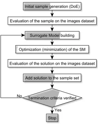
of an inference intelligence able to predict the objective function value of an unsampled solution to guide the search process. In the literature, such rep-resentation of the BB function it is referred to as the Surrogate Model (SM, see [20]) for which a large number of types and formulations were proposed. As frequently done in the recent literature the SM is used within a Sequen-tial Approximate Optimization (SAO) algorithm that iteratively updates the SM by adding the solution points that are determined at each iteration. This sequential approach preserves a certain simplicity but provides some impor-tant advantages. First, the rebuilding of the SM in order to capture the incoming information improves its reliability at each iteration. Second, it guarantees to perform a global optimization over the entire solutions do-main, by reducing the possibility to being trapped into local optima. The general scheme of the simple SAO algorithm we adopted is depicted in Figure 3.1.
The algorithm starts with the identification of the initial sample of so-lution points, used to initialize the SM. Then, for each sample point, the corresponding value of the objective function F (~x) in (3.1) is computed by applying the parameter values associated with the point to the CVA over the entire images test set. The incumbent solution is defined as the best solution found so far, hence it initially corresponds to the best sample. The SM is built from the current set of points (~x, F (~x)) and used to determine the next
Figure 3.1: Outline of the Sequential Approximate Optimization Algorithm
candidate solution. After this, the SM is interrogated in order to search for the best candidate solution possibly improving the incumbent. This phase is generally called adaptive sampling criteria. The process is iterated until termination criteria based on solution quality and running time are met.
As to the type of SM used, in this work due to the BBO nature of the problem we adopted a specific type of the so called Meshfree methods, named Radial Basis Function (RBF) interpolation techniques. These are relatively easy to construct and are widely used to approximate Black Box function responses. In RBF interpolation the model, s(~x), is defined as the sum of a
given number K of radial functions φ: s(~x) = K X J =1 γjφ(k~x − ~¯xjk) (3.2)
where ~xj, j = 1, ·, K, is the set of sampled solution points representing the
centers of the radial functions φ(), γ is a vector of weights to be determined, and ~x is the unsampled point whose value has to be predicted. Regarding the radial functions φ, several type are available in literature, varying from parametrized to not parametrized ones. In our case, the best trade off be-tween a simple construction of the SM and an acceptable reliability resulted with the use cubic basis function, that assume the form:
φ(k~x − ~xjk) = k~x − ~xjk3 (3.3)
We refer the reader to [21] for an overview of Meshfree methods, and to [22] for an example of industrial use of cubic RBF.
As to the initial sample generation through which initialize the SM, sev-eral techniques exists in literature, typically referred to as Design of Exper-iment (DoE). Since in our problem the parameters xj are not subject to
other constraints besides the upper and lower bounds, classical DoE as the Factorial Design are suitable. In particular, a Full Factorial Design (FFD) permit to cover the entire domain space, selecting all the points of the grid
generated by the discretization of each design variable (i.e., the parameters in our problem). This methodology is appropriate with the cubic RBF in-terpolation since it guarantees a sufficient reliability only inside the convex hull of the sampled points. However, in our case the computation of F (~x) is extremely time-consuming and using grids in which the parameter’s values are discretized is not practically possible. For this reason, we decided to initialize our algorithm through a |I|2 FFD, using just the domain vertices obtained with the lower and upper bounds of the parameters to be optimized. To improve the initial sample quality we also considered an initialization in which H additional random points selected inside the domain hypercube are considered. The adaptive sampling strategy that we adopt to perform the search of the candidate solution on the SM is the minimization of its pre-dictor s(~x). To avoid to being trapped in a local minimum and perform an efficient search over all the domain, we implement a multi-start gradient de-scent algorithm and run it by using a discrete grid of starting points.
Finally, we terminate the algorithm after a maximum number of objective function evaluations or after a given number of non-improving iterations.
3.4
Experimental Validation
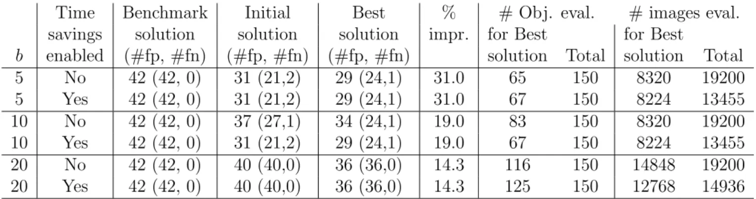
We applied our algorithm to the tuning of a CVA used to detect a specific type of defects on tyre images obtained in a real-world production environ-ment. The training set is made up of 160 images for which the presence or absence of defects is known. Six parameters were selected as the target for the optimization. Each such parameter has a maximum and minimum value and a default value manually determined by the CVA designers. The behav-ior of the CVA with the default parameter values is used here as a benchmark reference to evaluate the performance of the optimized parameters set.
We tested the impact of three variants for the initialization step, leading to three different overall algorithms A1, A2, and A3. In A1 we used H1 = 100
random points to initialize the algorithm. In A2 the sample set is constituted
by the 26points of the simple FFD described in Section 3.3. Finally, in A3, we
added to the FFD set H3 = 36 random internal points. The overall algorithm
is run for a total of 200 objective function evaluations (including those for the initialization step). The gradient descent search for the candidate solution is performed from a 96 discrete grid of points.
To account for possible different relative importance of false positives and false negatives in the defect detection, we considered two different pairs of weights in the objective function (3.1). Namely, we considered (αp, αn) =
{(1, 5), (1, 10)}.
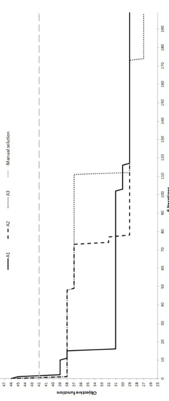
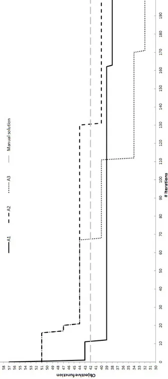
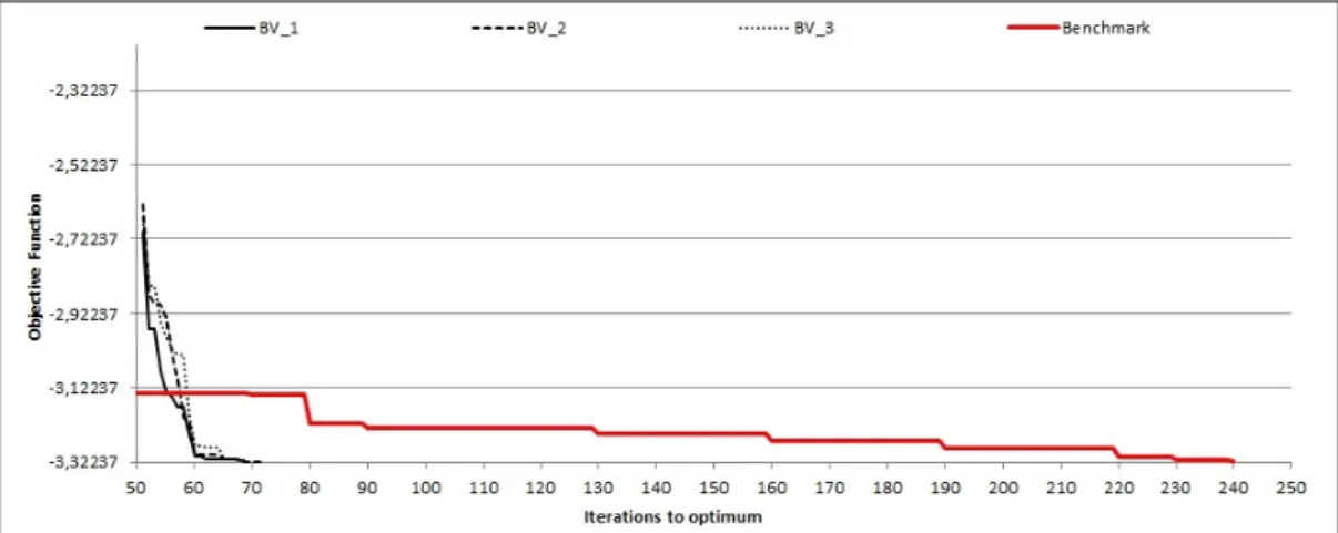
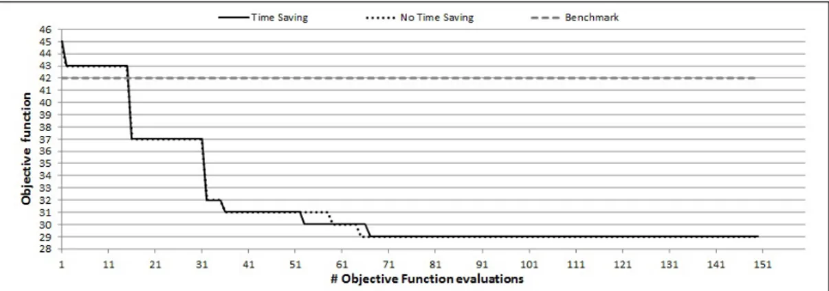
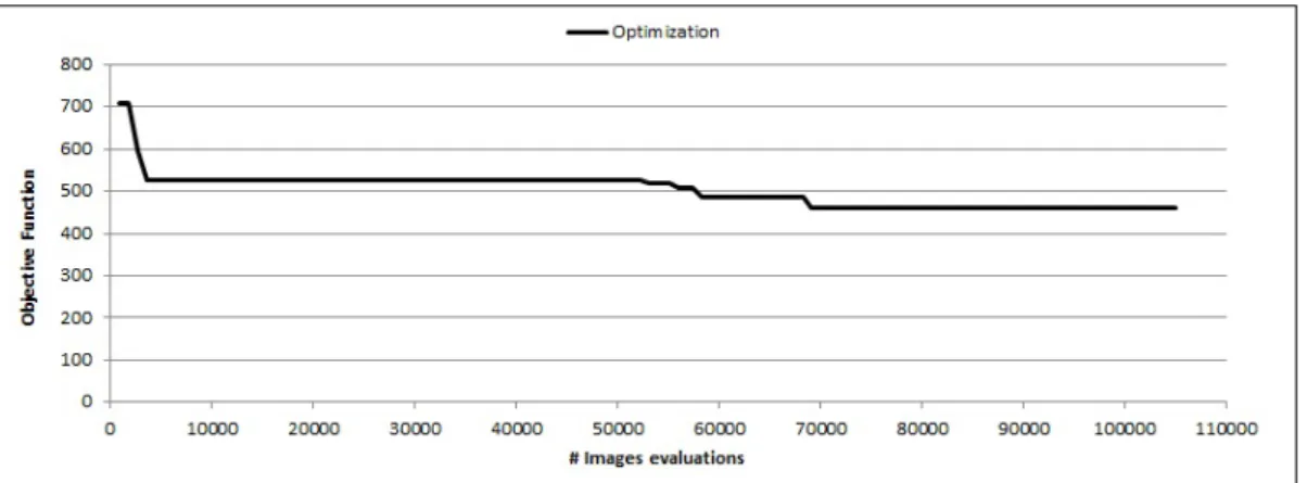
The results for the three algorithms are illustrated in Figures 3.2 and 3.3 for the (1,5) and (1,10) weight combinations, respectively. The figures report the evolution of the objective function for each algorithm compared with the benchmark reference equal to 42 for both weight combinations. By observing the figures it clearly appears that all proposed algorithms generate better parameter combinations with respect to the manual ones. In particular, for the (1,5) case A1, A2 and A3 produce solutions with value 29, 29 and 27,
respectively, which are 31% and 36% better that then manual ones. For the (1,10) case, they find a solution with value 38, 40 and 32, which are 10%, 5%, and 24% better, respectively. In general, we can observe that the mixed initialization of A3 provides better final results but the simple FFD of A2
improves quite rapidly and may constitute a good alternative when less time is available.
Figure 3.2: Evolution of the proposed algorithms with weight combination (1,5) in comparison with the manual tuning.
Figure 3.3: Evolution of the proposed algorithms with weight combination (1,10) in comparison with the manual tuning.
Chapter 4
Parameter Tuning of Computer
Vision Algorithms Through
Sequential Approximate
Optimization
4.1
Introduction
In this chapter, we address the optimal calibration of Computer Vision Al-gorithms (CVAs) used in the automated defect detection of pieces produced by an industrial plant. The final quality control check at the end of the
pro-duction chain consists in the optical scan of the produced pieces by a set of several CVAs. Each of them is designed to detect a specific type of defect and its behaviour is controlled by a large set of parameters controlling various aspects, such as the image noise filtering and the edge detection capability. Given an image of the piece to be checked, obtained with an appropriate camera, the CVA returns a binary value indicating if it is judged as defected or not. For a general introduction to defect detection and the use of com-puter vision, see [23]. The various parameters influence the CVA sensibility and accuracy, and must be optimally determined in order to maximize its detection efficacy on specific types of images. As in many other applications, the parameter tuning of the CVAs is, therefore, a crucial component for the overall efficacy of the system. Given a set of test images, the efficacy of the defect detection is measured as a function of the false positive and false negative detection ratios produced by the CVA with a specific parameter set. Its computation requires the application of the CVA to each image of the set, which is typically a very time-consuming operations requiring from seconds to minutes per image. Therefore, approaches based on expensive black-box optimization (see, e.g., [24] and [11]) must be used in this case. The presence of constraints between parameters and their possible integer type represents further complicating factors. In the literature, there are some general approaches to the parameters optimization of generic software,
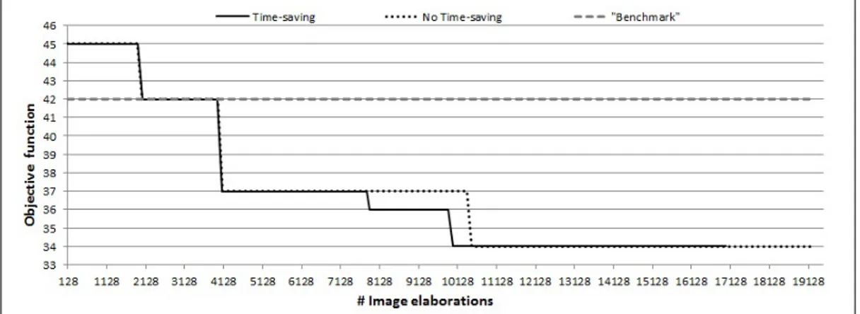
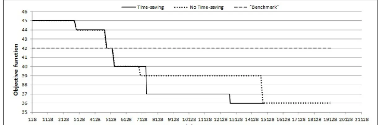
as illustrated, for example, by [13]. An early example of a CVA parameter tuning approach, limited to few parameters in an unconstrained continuous domain, can be found in [25]. However, to the best of our knowledge, no CVA optimization method able to handle all the issue presented by our specific application has been developed so far. We then developed a sequential surro-gate based optimization algorithm to identify the optimal parameter values to be applied to a CVA used to detect a specific defect on the images. During the optimization process, each parameter solution iteratively found by the algorithm is evaluated by comparing the CVA outputs obtained on the im-ages and their true defectiveness state, obtaining the true and false positive index ratio for the solutions tested. The set of the non-dominated parame-ters solutions give an approximation of the receiver operative characteristic (ROC) curve of the CVA. Since the various types of defects are very different both because of the different occurrence frequencies in the production chain and of the relative severity, every CVA must be optimized independently. Our goal is the determination, within a limited amount of computing time, of the optimal input parameter combination for a set of target-CVAs, leading the best possible false positive and false negative ratios for each particular type of defect. To reduce the large computing time required by the images elaborations, we developed an effective time-saving strategy that exploits the specific characteristic of the problem and is based on the partial elaboration
of the images dataset at each algorithm iteration. This paper is organized as follows. In chapter 4.2 we describe the characteristics of the problem under study. In chapter 4.3 we present a brief literature survey on the approaches we use in our solution algorithm: namely, the Black-Box Optimization and the main surrogate modeling techniques. The structure of the developed algorithm is presented in detail in Section 4, including the selection and vali-dation of a surrogate model based on Gaussian process regression to support the optimization process, and discussing how the constraints on the input variables and their possible integer nature can be handled. In Section 5 we discuss the results of an experimental validation of the algorithm on both an analytical benchmark from the literature and on data coming from a specific real-world application. Finally, in Section 6 we draw some conclusions and outline directions of future research.
4.2
Problem Description
The calibration of the parameters of a CVA is an optimization problem which can be described as follows. The variables to be optimized are the input pa-rameters of the CVA. Preliminary tests have shown a high responsiveness of the CVA’s behaviour even with respect to limited variations on the input variables, and the response of the CVAs to parameter changes has shown to
be multimodal. The variables associated with the parameters to optimize are associated with a range of variation (i.e., a lower and an upper bound) and are possibly subject to linear constraints on their values involving some pairs of them. Furthermore, even though some of the parameters may assume only discrete values, in the practical application that motivates our research typically the variation ranges of such discrete variables are large (even hun-dreds of values) and the CVA’s response to their variation can be considered relatively “smooth”. The performance of the CVA is measured in terms of two independent indicators, namely the number of negatives and false-positives in the solution, to be defined later. It can, then, be considered a Multi-Objective optimization problem. More specifically, since these indica-tors are not analytically predictable but can be only empirically measured by running the CVA with a specific set of parameters on a set of target images for which the presence of the defect is known, it is a Multi-Objective Black Bok Optimization problem.
More precisely, we have a CVA whose behaviour depends on a set H of pa-rameters. A subset I ∈ H of parameters are subject to the optimization while the remaining H \ I are fixed to a pre-determined value: in the follow-ing the fixed parameters will be no longer considered. For each parameter i ∈ I we are given lower and upper bounds li and ui, respectively as well as a
I is partitioned into two subsets I = Ic∪ Id, where Icis the set of continuous
parameters and Id is that of the discrete ones. Moreover, for each parameter
i ∈ I let xi be the decision variable which represents its value. Given solution
x we can evaluate its quality by measuring the performance of the CVA on a training set S of images. To this end, let f p(x) be the number of false-positives returned by the CVA when applied to the set S with parameters x, defined as the number of non-defective images which are classified as defective by the CVA. Similarly, let f n(x) be the number of false-negatives returned by the CVA, defined as the number of defective images which are classified as non-defective by the CVA. Note that such values represent two different objective functions depending on x which must be minimized. Therefore, the problem can be formulated as the following two-objective problem.
M in[f p(x), f n(x)] (4.1) subject to: xi > li ∀i ∈ I (4.2) xi 6 ui ∀i ∈ I (4.3) Ax ≤ c (4.4) xi integer ∀i ∈ Id (4.5)
Where constraints (2) and (3) impose the lower and upper bounds. Con-straints (4) represent the set of linear relations between the parameter values and (5) define the integer variables.
As frequently done in the literature the two-objectives problem is transformed into a single objective one by combining the two performance measures into a weighted sum of their values. Hence the objective function (1) becomes
M in[a ∗ f p(x) + b ∗ f n(x)] (4.6)
where a and b are the non-negative weights. Moreover, since the objective function value depends on the cardinality of the test set S and the associated defectiveness state, it can be normalized so that it takes only values between 0 and 1.
4.3
Overview of Black-Box Optimization
Ap-proaches
In this section, we briefly present the main approaches presented in the liter-ature for Black-Box optimization (BBO). A BBO problem is an optimization problem in which at least one function, typically the objective function, is a Black-Box function (BBF), i.e., a function that has the following properties:
• It is not expressed in analytical form. For example, because the func-tion represents the response to the input the variables of a system whose internal behaviour is unknown. This implies that the computation of its value can only be obtained thought an empirical experiment on the system.
• The computation can be time-costly, especially if the evaluation of system’s response consists in a physical experiment or in the run of a dedicated computer simulation software.
• The computation of the function may not return, in addition to its value, any other information of higher order such as the gradient. • The response of the system can be multimodal with respect to the input
variables.
• The response of the system can be affected by noise (i.e., it is a so-called a noisy Black-Box function).
There are several implications of the above-mentioned characteristics. For example, due to the lack of analytical description of the internal behaviour of the system, some kind of inference intelligence is necessary to select the can-didate solutions to be evaluated, based on those evaluated previously. Several types of inference intelligence and different criteria to select the new solution
to be evaluated exists, and some of them will be discussed later. More-over, the lack of higher order information, such as the gradient, increases the difficulty in the building of the inference intelligence, since it can be based on fewer information. A time-costly BBF evaluation implies that only a few evaluations can be done in a reasonable time, contrary to traditional optimization methods which rely on a huge amount of evaluations. Multi-modality, implies that the BBF is not convex, hence there is the possibility of not finding the global optimum and remaining trapped in local optima. As it is well described in [24], to perform global optimization in such multimodal condition it is necessary to perform both global and local search during the optimization process, indicated as exploration and exploitation. Finally, the presence of noise makes the response of the system is non-deterministic, i.e., it can vary from different evaluations even with the same input parameter values and this should also be taken into account by the inference intelligence.
We observe that in the practical application that motivates this paper, the BBF to be optimized is not affected by noise because it is obtained by run-ning on the test images the CVA, which is a deterministic computer code. Furthermore, the evaluation of the BBF through the CVA does not return gradient information, and is extremely time-costly requiring approximately 30 minutes per evaluation with the dataset used.
In the literature, there are several approaches to optimize single-objective Black Box Optimization problems. One way of classifying them is with re-spect to the type of the inference intelligence used. To this end, we can distinguish between approaches which either use or not a surrogate model (SM), see, e.g., [26]. A SM is a simplified representation of the BBF that describes the relation between inputs (i.e., the problem variables) and out-puts of the real system to be optimized, based on the values of the already sampled points. An SM can be built in several ways and, in addition to the function value at an unsampled point, the SM permits to infer different infor-mation about the real system, such as the associated prevision error, which can be used to better choose the next point to evaluate. The use of an ap-propriate SM can greatly reduce the number of evaluations to be performed during the optimization process. On the other hand, when no SM is used, the optimization is performed through techniques that, to select the next point to be evaluated, use only the values obtained from the sampled points of the real system. General approaches not using SM such as, for example, Genetic Algorithms or Direct Search (see, e.g., [26]), require a much larger number of evaluations of the BBF, which makes these techniques impractical when the BBF to optimize is time costly, as it is in our case. Therefore, we concentrate on SM-based approaches only. In the following, we examine
the different components of such methods. In particular, we first address the strategy to select the initial set of points used to build the SM and then we consider the SM building techniques. We next address the validation of the SM and its optimal tuning in order to guarantee its higher possible reliability. Finally, we describe the optimization process which includes the search of the next candidate solution through the so-called adaptive sampling criterion, and discuss the stopping criteria.
4.3.1
The selection of the initial set of points
The common technique used to select the initial sampling points is called Design of Experiments (DOE). As explained in [27], the DOE aims at al-locating sample points across the design space to maximize the amount of information derived from the real system. Classic DOE methods were devel-oped to support physical experiments and control the effects of the associated random errors. The main example of such methods is the so-called Factorial design, whose principle is to discretize each of the d design variables into n values and then select the points from the resulting hyper-grid. Whenever all the resulting points are considered, we have the so-called Full Factorial Design (FullFD) and their number is equal to nd, with n usually small and
sample space is represented by selecting only a subset of them, leading to the so-called Fractional Factorial Design (FractFD). Other examples of clas-sical DOE methods are the Star Design (SD), where a central point and two points for each design variable, usually corresponding to the lower, upper or average values, and the Central Composite Design (CCD), which combines SD and either FractFD or FullFD. Modern DOE methods were developed to mainly support deterministic experiments unbiased by noise such as the run of computer code, as it is in our case. The most used ones are known as Latin Hypercube Sampling (LHS), Orthogonal Array Design (OAD) and Uniform Design (UD). In LHS the points are sampled randomly in the design space but, each design variable is discretized into n values, and points are selected within this hyper-grid so that for each one-dimensional projection over each variable, there is only one point for each of its n values. LHS is easy to im-plement, but may provide non-uniform distributions of points, hence OAD and UD are extension trying to achieve a more uniform distribution of the sample points. We refer the reader to Giunta (2003) for a complete review of modern DOE techniques. We note that all such methods assume that the design space is a hypercube only bounded by upper and lower bound con-straints on the design variables.
When, as it is our case, additional constraints on the variables are present, such methods became not applicable. To address this, other methods were
proposed in the literature and are often referred as Space-Filling Design (SFD). SFD methods guarantee a good uniform distribution of points over a highly constrained convex domain. Their core mechanism is that points are iteratively moved in the space by optimizing a given distance measure such as, for example, by maximizing the minimum distance between each pair of design points. In this case, the SFD is called the MaxMin Design. If instead the objective is to minimize the distance of each points of the domain from the nearest SFD point it is called MinMax Design. Finally, several ways were proposed in the literature to decide how to move the points, that range from geometrical techniques to physics-inspired principles. For a survey on SFDs, we refer the reader to [28]. Given the nature of our problem, we de-cide to develop a simple but efficient MinMax SFD which will be described in Sect. 4.4.1.
4.3.2
The surrogate model building technique
Different types of surrogate model building techniques were proposed in the literature (see [27]), which can be classified into either Physical Surrogates (PS) or Functional Surrogates (FS). The construction of a PS typically as-sumes that some information of the internal structure of the system to model is known. In this case, the main technique to build the PS is to use a
sim-plified representation of the system. For example, by using either a coarser discretization when a simulation software is used to obtain the values of the system response, or a simplified analytical form of the relevant physics laws. PSs are generally easy to design but computationally expensive to be evalu-ated and typically not adaptable to other systems. In the case we consider in this paper, a PS is clearly not usable since the system to describe is actually a CVA.
An FS technique uses a mix of algebraic and statistical models to represent the response of the real system. They do not require any knowledge about it, since its behaviour is implicitly represented by the coefficients of the model which are iteratively tuned. This feature make FSs generic and not bounded to the specific target system. Instead, the correct choice of the coefficients, beside the optimal selection of the algebraic model, represent a critical step in their use. In fact, the definition of the coefficients is carried out by sam-pling and fitting procedures. Starting from an initial set of sample points, defined through the DOE techniques already described, during a fitting step the coefficient values of the model are chosen so that they provide the best fit of the current set of points. It is then clear that the suitability of the FS in representing the real system is strictly dependent on the selection of an appropriate sampling strategy.
Several different mathematical forms have been used as FS models to ap-proximate the unknown behaviour of the system (see, e.g., [29]), most of which are known as Response Surface Methodologies (RSM). For example, non-interpolating techniques include Polynomial Regression (PR) and Ra-dial Basis Function (RBF) approximation. In such cases, the response of the model does not coincide with that of the real system at the sampled points and the model structure and coefficients are chosen so as to provide a simple functional structure that minimizes the sum of squared error with respect to the actual model response at the sampled points. In PR the model is actually a polynomial of given degree for which the coefficients have to be chosen, while in RBF approximation the model, s(x), is defined as the sum of a given number k of radial functions ϕ(·):
s(x) =
k
X
j=1
γjϕ(k x − cj k) (4.7)
where cj, j = 1, ..., k is the set of centres of the radial functions and y = [y1...yk]T is a vector of weights to be determined. Generally, k is smaller
than the number of sample points and several types of radial functions are used in practice such as cubic, splines, Gaussian and Multiquadric functions. As to the interpolating techniques, the model is constructed so that its re-sponse coincides with the value of the sampled points of the real system. To
this end, the centres of the RBF coincide with the sampled points and the order of the model grows with the sample size. It is easily seen that inter-polating techniques are applicable only if the system response is not affected by noise.
A particular family of interpolating methods is represented by the Gaus-sian Process Regression (GPR), also known as Kriging, which is one of the most widely used approach in the literature. GPR is based on the assump-tion that, even if the response of the system is deterministic, it can be viewed as the realization of a stochastic process. The core principle in predicting the response value at an unsampled point x is to use the previously performed evaluations to identify the value that is more consistent, under specific statis-tic assumptions, with the sampled data. Due to the fact that estimating of the model parameters can be computationally costly, the building of GPR require more effort compared to the other methods. However, several papers prove that GPR generally provide better system approximation. For a com-plete review of non-interpolating and interpolating techniques in SM building the reader is referred to [11] and [29]. Our optimization problem is character-ized by a noise-free response and by a highly time-consuming computation. The first feature makes interpolating techniques usable. The second highly reduce the number of response evaluation (i.e., sample points evaluations)
that can be performed in the given time. For these reasons, we have chosen the GPR as SM building method, and we will describe our implementation in Sect. 4.4.2.
After the initial SM is built, a check of its reliability is often performed to verify if it is appropriate for the specific application. Also in this case, several techniques have been developed, among which the most used class is that of Cross Validation (CV) techniques. Here, the dataset of known samples of the system is split into a training set and a test set, then the first is actually used to build the SM, while the second is used for its valida-tion by comparing the values of the SM predicvalida-tions with the actual values of the system, thus obtaining relative and absolute errors. Depending on the ways in which the two sets are defined several assessment procedures can be defined, such as the Exhaustive CV, where all the possible ways to divide the original set must be tested and the corresponding indicators collected, or the Leave-One-Out CV (LOOCV), where the test set is made up by a single element chosen from the sample. If the assessment of the SM reliability is not satisfactory, different strategies exist to improve it. If the SM present parameters than can be tuned, like in parameterized RBF interpolation or in GPR, the model can be rebuilt by varying its parameters and trying to improve the LOOCV performance. Obviously, such attempt is not possible
if either the parameters are fixed during the initial building of the model, or if model parameters are not present. In this case, the possible strategy is to enlarge the training set. To this end, new points of the real system are chosen in such a way to achieve the maximum augment of the SM reliability according to a so-called infill criteria. In Sect. 4.4.3 we explain the strat-egy we developed to efficiently tune the parameters of the GPR model we implemented and to measure its reliability.
4.3.3
The search strategy for the candidate solution
The methods used to search the optimal solution within the SM built are commonly called adaptive sampling methods, and the most common ones are so-called two-stage approaches. Here, the SM is first built by using the existing samples and estimating all the required parameters of the model. Then, the search of the optimal solution is performed over the resulting re-sponse surface, that is densely searched. Several search strategies exist, and their usability depend on the type of SM used. The main discriminant is associated with the use or not of a stochastic approach such as the GPR in building the SM. In the negative case we cannot obtain information about the standard error associated to the predictor, then the only applicable ap-proach is the Minimization of the Response Surface (MRS), which consists
in exploring the response surface to find its global minimum, for example through a gradient descent algorithm coupled with a multistart mechanism to reduce the probability of being trapped into a local optimum. Instead, whenever the SM provides information about the standard predictor error, various methods using such error of it are available, where the Maximization of the Expected Improvement (MEI) represents the most common one. The adaptive sampling strategy that we implemented is described in Sect. 4.4.4.
4.3.4
The overall search process
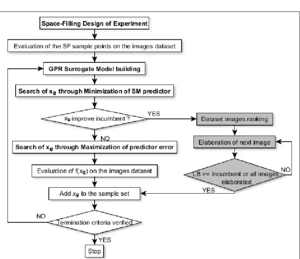
Surrogate-based optimization processes may be either one-shot or iterative, where in the latter, known as Sequential Approximate Optimization (SAO, see [19]), the SM is iteratively rebuilt, updated and used several times. SAO approaches clearly are more time consuming but generally obtain much better solutions than one-shot methods being able to perform global optimization in highly multimodal or noise-affected contexts. The process starts with a given sample of points tested on the real system, selected through a specified DoE. Then, the SM is built through a specific model-building technique, such as RBF or GPR, and is validated. If the model reliability is found unsatisfac-tory, the model parameters are tuned or new points to test are selected by a proper infill criteria, until a satisfactory reliability is achieved. An adaptive
sampling criteria is used to find the candidate solution to test, for exam-ple by using the MRS or MEI methods previously described. To achieve a global optimization, the adaptive sampling criterion used must balance Ex-ploitation and Exploration components. The former component is aimed at improving the incumbent by intensifying the search in its neighborhood, thus incurring the risk of remain trapped in local minima. The second component instead aims at exploring the under-sampled regions of the solution space. The candidate solution found is then evaluated on the real system and the incumbent is possibly updated. The solution found is finally added at the samples set, and the SM is rebuilt and the process is iterated until a stop criteria is met.
4.4
The Implemented Algorithm
We now describe the implemented algorithm and the way in which we have handled the major difficulties of the problem at hand, which are summarized as follows:
• High cost of the single point evaluation, due to the fact that the single solution’s evaluation is performed by running the target CVA on a large dataset of images.
• Presence of integer variables;
• Two different objective function to minimize: false positive and false negative index ratio.
• High multi-modality of the system response.
Being a time-costly BBO problem, we do not apply direct optimization to the system response. In fact, because gradient information is not available, the only possible direct optimization approaches are Derivative Free methods such as Genetic Algorithm or Direct Search, that require a large number of evaluations to produce satisfactory results and, in our case, could require an impractically large computing time. Hence, we developed an optimization algorithm based on a Sequential Approximate Optimization approach which experimentally proved to obtain very good results within an acceptable com-putational time. In the following, we describe in detail the component of the implemented approach following the scheme outlined in Sect. 4.3.
4.4.1
A space-filling Design of Experiment
As seen in Sect. 4.3.1, the main goal in the initial DOE is the selection of n points of the solution space in such a way to extract as much information as possible from the real system to optimize. The choice of the DOE is clearly crucial for the construction of the initial SM and thus for the overall efficiency
of the SOA method.
We developed a Space Filling DoE that iteratively allocates an arbitrary number n of points in the given convex domain so that they are as much uniformly dispersed in the domain as possible. More specifically, we imple-mented a MaxMin SFD (MmSFD), instead of a MinMax one, because it guarantees a more uniform sampling thanks to the minimization of the size of the “unsampled regions” and, at the same time, is able to easily han-dle the domain constraints. As to the integrality constraints, our MmSFD procedure enforces the sample points chosen to be integer. The principle according which the MmSFD works is the simulation of the behaviour of a particles system. Each point is associated with a particle with given mass we assume the presence of repulsive forces between every pair of particles, proportional to their distance. In addition, every point is subject to an or-thogonal repulsive force from each hyperplane supporting a cosntraint of the domain (including the lower an upper bound constraints). This avoids that a point violates the domain constraints, since the repulsive force became expo-nentially larger when the distance of the point from a constraint decreases. For each point, the direction and distance in which it should be moved is computed by considering the resultant of all the forces applied to it. At each iteration, all points are moved and the process is repeated for a given number of iterations. Let F be the complete set of linear constraints bounding the
domain including the lower and upper bound constraints on each variable corresponding to a parameter to be tuned. Moreover, let us assume for sim-plicity that the domain is limited and that all parameters are continuous. The procedure can be easily modified to account for integrality conditions on some parameters. The procedure starts by randomly generating n sample points into the domain, denoted as pt, t = 1, . . . , n.
At each iteration, for each point pt, t = 1, . . . , n, (called target point) we
compute the resultant of the repulsive forces between the point pt and all
other points ps,with s 6= t as well as all the constraints in F , by considering
the orthogonal projection of pton each of the constraints in F . As previously
mentioned, the repulsive force is inversely proportional to the distance be-tween the points, normalized with respect to the maximum distance bebe-tween two points in the domain. More precisely, the repulsive force between ptand
another point ps (i.e., both a sample and a projection over a constraint) is
defined as:
fs,t= (
dmax
k pt− ps k
− 1)h (4.8) where dmax is the maximum distance between two points in the domain
and h is a suitable parameter, typically set to a value ≥ 2 to ensure a fast convergence of the procedure. Once all repulsive forces are computed, their resultant is computed for each point which is moved in that direction by a
distance proportional to the force intensity, suitably scaled down n so as to avoid that two points exchange their relative positions as an effect of their movement.
The process is iterated until the position of the points become stable, e.g. when their coordinates do not vary by more than a predetermined threshold with respect to the previous iteration or after a given maximum number of iterations. As previously mentioned, if integer values of the variables are required these are obtained by a rounding step followed by a simple local search step where neighboring feasible integer points are evaluated.
4.4.2
The Surrogate Model
To define our Surrogate Model (SM) we first need to define precisely the objective function which represent the response value of our system. More precisely, we used equation (6) which allows us to treat the multi-objective BBO as a single-objective one and we normalized it by considering the max-imum number of false positives and false negatives in the training set. This allows to compare the objective function values also when different training sets are used to evaluate different points.
The specific SM we used in our implementation is a GPR interpolating SM, introduced in Sec. 4.3.2. In a GPR, the value of the response y(x) at a
sam-ple point x is considered as the realization of a Gaussian variable Y(x) with mean µ and variance σ2. All the variables Y are then assumed to be corre-lated to each other, and the correlation is expressed as a parametric function of the distance of the respective sample points. Several types of such func-tions were proposed in the literature for GPR, all based on an exponentially decaying structure and here we use the following, well-known, one:
Corr(Y (xi), Y (xj)) = e
−r(xi,xj )2
a (4.9)
where r(xi, xj) is the spatial distance between two points (xi, xj), and the
parameter a determines how fast the correlation decreases with the increase of r. We refer the reader to [30] for its derivation. In our implementation, we used the weighted Euclidean distance
r(xi, xj) = v u u t d X l=1 (wl(xil− xjl))2 (4.10)
where wl representing the scaling factor for the l-th dimension. Since the
higher is the value of wlthe larger is the correlation decrease with the increase
of the distance on the l-th dimension, the vector w is a sensitivity parameter vector associated with the domain dimensions. Given the correlation matrix R defined according to 4.9 we can define the GPR predictor ˆy(x∗) for a target