CEFIN – Centro Studi di Banca e Finanza
Dipartimento di Economia Aziendale – Università di Modena e Reggio Emilia
CEFIN Working Papers
No 9
Indebtedness, macroeconomic conditions and banks’ loan losses:
evidence from Italy
by S. Castellani, C. Pederzoli, C. Torricelli
Indebtedness, macroeconomic conditions and banks’ loan losses:
evidence from Italy
S. Castellani4, Pederzoli C.1,2, Torricelli C.1,3 ♦
1. Centro Studi Banca e Finanza (CEFIN), Università di Modena e Reggio Emilia
2. Dipartimento di Metodi Quantitativi per le Scienze Economiche e Aziendali, Università degli Studi Milano-Bicocca
3. Dipartimento di Economia Politica, Università degli Studi di Modena e Reggio Emilia 4. Independent
Abstract
The Basel II capital accord has fostered the debate over the financial stability of the aggregate banking sector. There is a large empirical literature focused on the effects of macroeconomic disturbances on the banking system. Specifically, loan losses are an important factor for the banking stability and a stream of research in this field aims to identify explanatory variables for this critical indicator.
This paper focuses on Italian banks data over the period 1990-2007 and investigates the relationship between the ratio of non-performing loans to total loans, the business cycle and firms’ indebtedness so as to test the impact of both real and financial fragility on banks’ default losses. We use a regression model with an interaction term representing the joint effect of real and financial fragility, which to our knowledge has never been applied before to Italian default data. The results show that the impact of financial fragility on default losses is enhanced by adverse economic conditions.
I. INTRODUCTION
The new Basel Capital Accord, known as Basel II (BCBS, 2006), has fostered the debate over the financial stability of the aggregate banking sector. Banks’ loan losses are an important factor for financial stability and hence a relevant stream of research has focused on analysing the determinants of losses.
In particular, it is well known that banks’ losses coming from borrowers’ default are affected by the economic conditions and this gives rise to concerns about procyclicality of capital requirements under Basel II. Additionally to a wide empirical literature (e.g. Bangia et al. (2002), Altman et al. (2002) among many others), the dependence of credit risk factors on business cycle is analysed in Allen and Saunders (2003), who provides a survey of cyclical effects in credit risk models.
The empirical literature testing the relation between banks’ performances and the business cycle is huge; some authors (e.g. Leaven and Majnoni (2003), Ayuso et al. (2004) among others) focus on provisions through the business cycle while others consider realized default losses. Among the letters, Sales and Saurina (2002) find an important contemporary impact of economic cycle on bad loans on Spanish data. Gambera (2000) identifies a set of macroeconomic variables (bankruptcy filings, -farming- income, state annual product, housing permits, and national unemployment) as predictors for problem-loan ratios on US data. Hoggarth et al. (2005) document the link between the UK business cycle and banks’ write-off. Quagliariello (2007), Quagliariello and Marcucci (2007) and (2008) analyse Italian data within different econometric frameworks (panel data on 1985-2002 annual bank specific data, threshold model on 1990-2005 quarterly aggregate data, and VAR on 1990-2004 quarterly aggregate data respectively) and focusing on the relation between business cycle and default rates. Pesola (2005) and (2007) analyse the impact of macroeconomic shocks on banks’ losses on European countries, paying particular attention to the Nordic countries. In particular, these two works consider macroeconomic variables and financial fragility as explanatory variables in a non-linear model: the final aim in this case is the understanding of factors causing banking crises.
In the same spirit as Pesola (2005) and (2007), we aim at analysing how real as well as financial conditions impact banks’ loan losses. We apply a comparable model to Italian data, considering a real variable, a financial variable and their interaction as explanatory variables for losses.
The paper is structured as follows. Section II explains the rational for the econometric model adopted. Section III presents the data and Section IV discusses the empirical results and compare them with the existing empirical literature. Section V concludes and provides some directions for further research.
II. THE ECONOMETRIC MODEL
The aim of this work is to analyse some critical determinants of banks’ loan losses at an aggregate level. The dependent variable, the banking system loan losses, is defined as a percentage of total loans (DR). We are interested in analysing the impact of economic and financial conditions on losses: in line with Marcucci and Quagliariello (2007), we measure economic conditions by means of the difference between actual GDP and its linear trend (GDPT) and we interpret it as a measure of ‘real fragility’. Moreover, in line with Pesola (2005), we consider the ratio of total loans to GDP (INDEB) as a measure of financial fragility, since the banking system is fragile when borrowers have high debts (i.e. high loans) compared to total output.
In order to test the hypothesis that both real and financial fragility affect banks’ loan losses, we use three nested models. We start with the simplest model based on the relation between GDP and default losses: the model is presented in equation (1), where DR is the percentage aggregate loss, GDPT is the deviation of GDP from its linear trend and e is the error term.
t t
t GDPT e
DR =α +β1 −1+ (1)
Consistently with previous studies, we expect a negative coefficient β1 since lower GDP values,
i.e. recessionary regime, determines higher default losses1.
Second, we define in equation (2) a regression model to capture how the two variables representing real and financial fragility affect the evolution of the banks’ loan losses. The regressors are both one period lagged.
t t t t GDPT INDEB e DR =α +β1 −1+β2 −1 + (2)
We assume that financial fragility (INDEB) positively affects default losses.
Thirdly, we define in equation (3) the model with the interaction term of financial and real fragility. t t t t t t GDPT INDEB INDEB GDPT e DR =α +β1 −1+β2 −1 +β3 −1⋅ −1+ (3)
The model in equation (3) allows to consider the joint effects of the real and the financial explanatory variables. Pesola (2005) proposes a model with joint terms only: in this work we aim to catch both the linear effect of each explanatory variable and the effect of each variable conditional to the other. Indebtedness may affect default loss depending on the specific GDP value: namely, we expect greater sensitivity to indebtedness during a recession, since the impact of financial fragility on default losses is enhanced by real fragility. This means that we expect a particularly high loss rate when both the indebtedness is high and GDP is low.
III. DATA
The models presented in Section II are estimated over Italian quarterly data spanning over the period 1990Q1-2007Q2. We use data from two sources: the Bank of Italy Statistical Bulletin for loans and default data for Italian non-financial borrower firms, the ConIstat for GDP data. The dependent variable DR is computed as the ratio of the flow of new defaulted debts in the reference quarter to the stock of performing loans of the previous one2. The explanatory variable GDPT is quantified by real (seasonally adjusted) GDP while the variable INDEB is obtained as the ratio of outstanding loans over nominal (seasonally adjusted) GDP.
Since data from the Bank of Italy are available both at aggregate level and separately by different categories, we exploit the distinction of firms by loan size to define two groups representing
2 The Bank of Italy database provides historical series of total and non-performing loans both in terms of number
and monetary amounts: in order to model the loss rate and the financial fragility variable, we used the latter measure. Moreover, in order to define the loss rate we should consider the recovery rates as well as the data on defaults. As a proxy we use the default data only, so that the variable LR is quantified as the aggregate default rate. The variable is the same used in Marcucci and Quagliariello (2007).
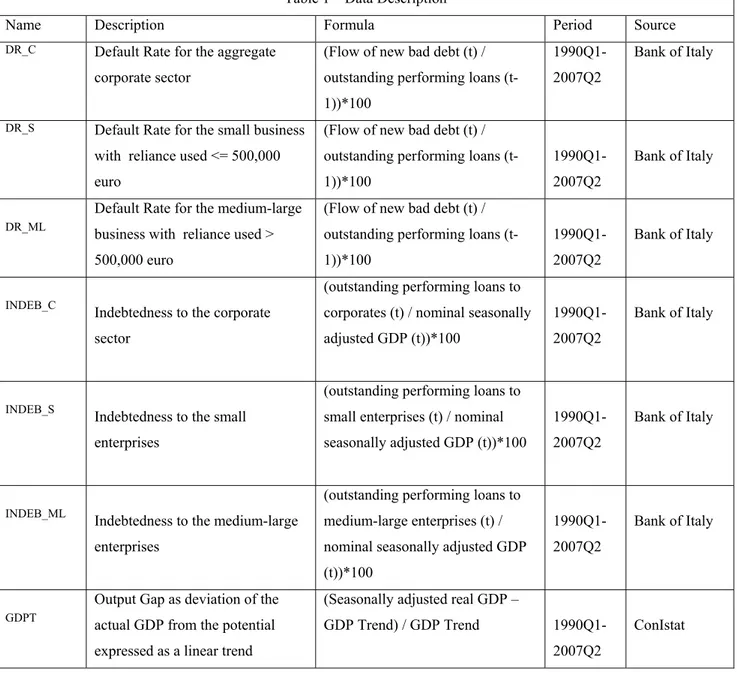
small and medium-large enterprises respectively3. Table 1 sums up the variables employed in the paper as for their construction and source.
Table 1 – Data Description
Name Description Formula Period Source
DR_C Default Rate for the aggregate
corporate sector
(Flow of new bad debt (t) / outstanding performing loans (t-1))*100
1990Q1-2007Q2
Bank of Italy
DR_S Default Rate for the small business
with reliance used <= 500,000 euro
(Flow of new bad debt (t) / outstanding performing loans (t-1))*100
1990Q1-2007Q2
Bank of Italy
DR_ML
Default Rate for the medium-large business with reliance used > 500,000 euro
(Flow of new bad debt (t) / outstanding performing loans (t-1))*100
1990Q1-2007Q2
Bank of Italy
INDEB_C Indebtedness to the corporate
sector
(outstanding performing loans to corporates (t) / nominal seasonally adjusted GDP (t))*100
1990Q1-2007Q2
Bank of Italy
INDEB_S Indebtedness to the small
enterprises
(outstanding performing loans to small enterprises (t) / nominal seasonally adjusted GDP (t))*100
1990Q1-2007Q2
Bank of Italy
INDEB_ML
Indebtedness to the medium-large enterprises
(outstanding performing loans to medium-large enterprises (t) / nominal seasonally adjusted GDP (t))*100
1990Q1-2007Q2
Bank of Italy
GDPT
Output Gap as deviation of the actual GDP from the potential expressed as a linear trend
(Seasonally adjusted real GDP –
GDP Trend) / GDP Trend
1990Q1-2007Q2
ConIstat
Figure 1 graphs the main variable employed in this study over the business cycle phases, based on the OECD turning points dates. Looking at the GDPT graph the negative peak in 1992-1993 is clearly the outcome of an unfavourable economic period after the European Monetary System
3 In order to distinguish between small and medium-large companies, the amount of credit drawn is used as a proxy
for the firm size; this criterion is also taken by other authors (e.g. Sironi and Zazzara 2003). In this work, in order to exploit the categories in the public database of the Bank of Italy, we define an obligor to be a small company when the credit used is less than 500,000 euro, while the company is considered a medium-large one when the credit used exceeds this threshold.
crisis and the peak in 1995 reflects the crisis of the Southern banking system (see e.g. Marcucci and Quagliariello, 2008). The strong recession in 1992-1993 is clearly associated to high default rates. Fig. 1 Data 0,1 0,3 0,5 0,7 0,9 1,1 1,3 1,5 1,7 1990 /1 1991 /1 1992 /1 1993 /1 1994 /1 1995 /1 1996 /1 1997 /1 1998 /1 1999 /1 2000 /1 2001 /1 2002 /1 2003 /1 2004 /1 2005 /1 2006 /1 2007 /1 DR_C 0,3 0,4 0,5 0,6 0,7 0,8 0,9 1 1,1 1,2 1990/ 1 1991/ 1 1992/ 1 1993/ 1 1994/ 1 1995/ 1 1996/ 1 1997/ 1 1998/ 1 1999/ 1 2000/ 1 2001/ 1 2002/ 1 2003/ 1 2004/ 1 2005/ 1 2006/ 1 2007/ 1 DR_S 0,1 0,3 0,5 0,7 0,9 1,1 1,3 1,5 1,7 199 0/1 199 1/1 199 2/1 199 3/1 199 4/1 199 5/1 199 6/1 199 7/1 199 8/1 199 9/1 200 0/1 200 1/1 200 2/1 200 3/1 200 4/1 200 5/1 200 6/1 200 7/1 DR_ML -3 -2 -1 0 1 2 3 4 1 9 90/1 1 9 91/1 1 9 92/1 1 9 93/1 1 9 94/1 1 9 95/1 1 9 96/1 1 9 97/1 1 9 98/1 1 9 99/1 2 0 00/1 2 0 01/1 2 0 02/1 2 0 03/1 2 0 04/1 2 0 05/1 2 0 06/1 2 0 07/1 GAPT 1,1 1,3 1,5 1,7 1,9 2,1 2,3 19 90 /1 19 91 /1 19 92 /1 19 93 /1 19 94 /1 19 95 /1 19 96 /1 19 97 /1 19 98 /1 19 99 /1 20 00 /1 20 01 /1 20 02 /1 20 03 /1 20 04 /1 20 05 /1 20 06 /1 20 07 /1 INDEB_C
Note: the colored bands on the background of each graph represent the recession periods according to the OECD
Descriptive statistics of the variables used and the relative correlation matrix are provided in the Appendix. Two different tests for stationarity are performed over the selected variables. First of all we employed the Augmented Dickey-Fuller (ADF) test which cannot reject the null of a unit root for the dependent variable (DR) and the financial fragility explanatory variable (INDEB). However, given the low power of ADF test in small sample, we applied the Kwiatkowski test (KPSS) as well: this test fails to reject the null hypothesis of stationarity at least at 1% for all the series involved in our main empirical analysis (see Section IV). Therefore, in the analysis, the variables included are all in level, keeping their original meaning.
IV. EMPIRICAL RESULTS
We first estimate the baseline model presented in equation (1): since we grouped corporates by small and medium-large firms, we estimate the same baseline model on the aggregate default rate and separately on the two groups’ default rates.
Table 2 – Baseline Model
1. Aggregate corporate sector 2. Small business sector 3. Medium-Large Corporate sector
α 0.650185 (0.057860) *** 0.644233 (0.034896) *** 0.654996 (0.063147) *** β1 -0.097713 (0.040492) ** -0.053005 (0.022622) ** -0.108916 (0.044881) ** R2 0.175451 0.159064 0.174873 Adj. R2 0.163145 0.146513 0.162558 F-Stat 14.25656 (0.000341) 12.67312 (0.000688) 14.19963 (0.000350)
Sample: 1990Q1 – 2007Q2 Method: Least Squares, Newey-West HAC Standard errors and covariance (standard errors are reported in brackets)*, **, *** confidence level respectively to 10%, 5%, 1%
1. Baseline model – Aggregate corporate sector - DR_Ct = α +β1GDPTt−1 +et 2. Baseline model – Small Business – DR_St = α +β1GDPTt−1+et 3. Baseline model – Medium/Large companies - DR_MLt = α +β1GDPTt−1 +et
The results of the estimation, reported in Table 2, confirm the well-known negative relationship between default rate and GDP. Small business are less dependent on macroeconomic conditions, being more affected by specific risks.
Once explained the baseline model, we focus on small corporates only, which represents the engine of the Italian economy covering the 99,92% of the total Italian enterprises4.
Table 3 shows the results of the regression model defined by equation (2): both regressors are significant and R2 is higher than the baseline model. The signs of coefficients are as expected: the coefficient on GDPT is still negative, while the coefficient on INDEB is positive as financial fragility increases default rates.
Table 3 Two regressors model α 0.644899 (0.030963) *** β1 -0.040854 (0.016989) ** β2 2.463000 (0.807940) *** R2 0.315949 Adjusted R2 0.295221 F-Stat (prob) 15.24204 (0.000004)
Sample: 1990Q1 – 2007Q2 Method: Least Squares, Newey-West HAC Standard errors and covariance (standard errors are reported in brackets)
*, **, *** confidence level respectively to 10%, 5%, 1 Small Business no interaction model:
DR_St = α +β1GDPTt−1 +β2INDEB_St−1+et
In order to capture the joint effect of the two regressors, we estimated the model defined in equation (3) which included the interaction term.
Table 4 Interaction model
α 0.643329 (0.031960) *** β1 -0.041143 (0.016987) ** β2 2.400064 (0.787990) *** β3 -0.179700 (0.443534) R2 0.317605 Adjusted R2 0.286109 F-Stat 10.08423 (0.000015)
Sample: 1990Q1 – 2007Q2 Method: Least Squares, Newey-West HAC Standard errors and covariance (standard errors are reported in brackets)
*, **, *** confidence level respectively to 10%, 5%, 1% Small Business no interaction model:
t t t t t t GDPT INDEB S INDEB S GDPT e S DR_ =α+β1 −1+β2 _ −1+β3 _ −1⋅ −1+
The regression coefficients reported in Table 4 have all the expected signs: the negative sign on the interaction term coefficient can be interpreted by rewriting equation (3) as follows:
(
2 3 1)
11
1 _
_St = + GDPTt− + + GDPTt− ⋅INDEB St−
DR α β β β (4)
By means of the interaction term, the slope coefficient of the variable INDEB on the loss rate can be seen as dependent upon the value of GDPT. By considering three particular values of GDPT, GDPTM, GDPTH, GDPTL, corresponding to the mean value of GDP and one standard deviation above and below the mean respectively, simple regression lines are generated by
substituting these values into the equation (4). The results5 are reported in Table 5. The slopes of the three regressions have the same sign: the difference between the three equations consists in the magnitude of the sensitivity of the loss rate to the indebtedness. The equation is steeper when the GDPT is negative: this means that an increase of indebtedness, in recessionary economic conditions, leads to a more intense increase of default rate than in expansionary phases, that is the impact of financial fragility on default losses is enhanced by the real fragility. The coefficient on the interaction term however is not significant and therefore we can only comment its meaning without a strong statistical support.
Table 5 Simple Conditional Regression Equations
(
2 3 1)
1 1 1 _ _St = + GDPTt− + + GDPTt− ⋅INDEB St− DR α β β β GDPTt-1= 1.333174 1 _ 1598 . 2 5877 . 0 _St = + ⋅INDEB St− DR GDPTt-1=0 1 _ 3994 . 2 6425 . 0 _St = + ⋅INDEB St− DR GDPTt-1= -1.333174 1 _ 6389 . 2 6972 . 0 _St = + ⋅INDEB St− DRPesola (2007) proposes an econometric model with interaction terms only6 , which is therefore not directly comparable with our estimation. He presents the estimation of the linear and the “combined model” as well: however in this case most of the variables turn out to be not significant.
It has to be noted that the Italian default rates are significantly lower on average in the last years: this can be associated to the publication of the January 2001 document of Basel II, which possibly led banks to adopt more severe credit standards and therefore to improve borrowers’ risk features. Therefore we introduce a dummy variable to control for the reduction in default rates from January 2001 on7. The results are reported in Table 6. The dummy is significant, confirming a reduction in default rates starting from 2001. Moreover, by controlling for the general credit quality improvement likely following the Basel II document, the interaction term
5 The introduction of the interaction term requires the continuous explanatory variables to be centred in order to
avoid distorsions in the coefficients of the single regressors coefficients (see Aiken and West, 1991).
6 Pesola (2007) estimates his model on annual data and its dependent variable is the actual loss rate. The regressors
are the product terms of macroeconomic shock and financial fragility and interest rates shock and financial fragility additionally to the lagged loss rate.
becomes significant (supporting the idea presented before) and the R2 significantly improves8.
Table 6 Interaction model with dummy
α 0.728784 (0.021976) *** β1 -0.025715 (0.010925) ** β2 1.735314 (0.555276) *** β3 -0.889328 (0.355931) ** γ -0.243729 (0.039117) *** R2 0.724467 Adjusted R2 0.707246 F-Stat 42.06919 (0.000000)
Sample: 1990Q1 – 2007Q2 Method: Least Squares, Newey-West HAC Standard errors and covariance (standard errors are reported in brackets)
*, **, *** confidence level respectively to 10%, 5%, 1% Small Business no interaction model:
t t t t t t GDPT INDEB S INDEB S GDPT D e S DR_ =α+β1 −1+β2 _ −1+β3 _ −1⋅ −1+γ 2001+
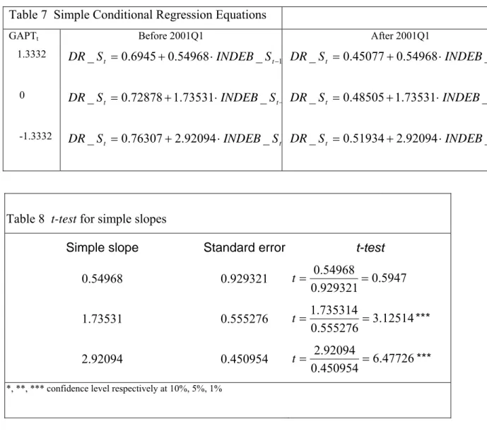
In particular, Table 7 presents the simple regression equations emerging from conditioning the default rate to three specific values for GDPT: the impact of financial fragility on the loss rate is clearly higher for lower GDP values. Moreover, the coefficient comes out to be strongly significant for negative GDPT values while it is not significant for positive GDPT (see Table 8): this stylized analysis suggests that indebtedness contributes to increase default rates only if combined with adverse economic conditions.
Table 7 Simple Conditional Regression Equations
GAPTt Before 2001Q1 After 2001Q1
1.3332 1 _ 54968 . 0 6945 . 0 _St = + ⋅INDEB St− DR DR_St =0.45077+0.54968⋅INDEB_St−1 0 _ 0.72878 1.73531 _ − ⋅ + = t t INDEB S S DR DR_St =0.48505+1.73531⋅INDEB_St−1 -1.3332 _ =0.76307+2.92094⋅ _ t t INDEB S S DR DR_St =0.51934+2.92094⋅INDEB_St−1
Table 8 t-test for simple slopes
Simple slope Standard error t-test
0.54968 0.929321 0.5947 929321 . 0 54968 . 0 = = t 1.73531 0.555276 3.12514 555276 . 0 735314 . 1 = = t *** 2.92094 0.450954 6.47726 450954 . 0 92094 . 2 = = t ***
*, **, *** confidence level respectively at 10%, 5%, 1%
V. CONCLUSIONS
The aim of this paper is to make a step forward in explaining the Italian banking sector’s aggregate loan default losses. The literature is rich of empirical papers focusing on the relation between business cycle and default losses, and a few papers analyse Italian data. In this work we analyse the Italian firms’ default rates over the period 1990-2007. In line with the model proposed in Pesola (2005), we consider the impact of both real and financial fragility. Moreover we consider the impact of the product term representing the interaction between real and financial fragility, which allows to quantify the impact of each explanatory variable conditional to the other. The basic idea behind the interpretation of the interaction is that indebtedness itself is a source of risk, especially if coupled with adverse economic condition.
relationship between the business cycle and Italian firms’ default rates over our longer time period and find a positive relation between financial fragility and default rates. Moreover, by considering the interaction term, which as far as we know has never been applied before to Italian data, we find a more intense impact of indebtedness when the economic conditions are unfavourable.
While we focused on default losses due to corporates credit extension (in particular small business), the next step is to analyse default losses due to the total of borrowers. This is important when considering the aggregate default losses as a source of banking crises.
REFERENCES
Aiken L.S. and West S.G. (1991), “Multiple Regression: Testing and Interpreting Interactions”, SAGE Publications, Inc., Newbury Park, California.
Ayuso J., Perez D., Saurina J., 2004. “Are capital buffers pro-cyclical? Evidence from Spanish panel data”. Journal of Financial Intermediation, 13, 249-264.
Allen L., Saunders A., 2003. “A survey of cyclical effects in credit risk measurement models”, BIS Working Papers, 126.
Altman E., Resti A., Sironi A., 2002. “The link between default and recovery rates: effects on the procyclicality of regulatory capital ratio”, BIS Working papers, 113.
Bangia A., Diebold F., Kronimus A., Schagen C., Schuermann T., 2002. Ratings migration and the business cycle, with application to credit portfolio stress testing. Journal of Banking &
Finance, 26, 445-474.
Basel Committee on Banking Supervision –BCBS- (2006), “International Convergence of Capital Measurement and Capital Standards”, Bank for International Settlement.
Gambera M. (2000), “Simple Forecast of Bank Loan Quality in the Business Cycle”, Federal Reserve Bank of Chicago, Supervision and Regulation Department, Emerging Issues Series, S&R-2000-3.
Hoggarth G., Sorensen S., Zicchino L. (2005), “Stress test of UK banks using a VAR approach”, Bank of England, Working Paper 282.
ISTAT (2007), “Structure and Dimension of the Enterprises”. Available at: http://www.istat.it/salastampa/comunicati/non_calendario/20070712_00/
Laeven, L., and Majnoni, G. (2003), “Loan loss provisioning and economic slowdowns: Too much, too late?”, Journal of Financial Intermediation, 12, 178-197.
Marcucci J and Quagliariello M. (2007), “Credit Risk and Business Cycle over Different Regimes”, Centre for Econometric Analysis CEA@Cass.
Marcucci J. and Quagliariello M. (2008), “Is bank portfolio riskiness procyclical? Evidence from Italy using a vector autoregression”, Journal of International Financial Markets, Institutions &
Money, 18 (1), 43-63.
Meyer A.P. and Yeager T.J. (2001), “Are small Rural Banks Vulnerable to Local Economic Downturn?”, Federal Reserve Bank of St. Louis Review, 25-38.
Pesola J. (2001), “The Role of Macroeconomic shocks in Banking Crises”, Bank of Finland, Discussion paper no. 6.
Pesola, J. (2005) "Banking Fragility and Distress: An Econometric Study of Macroeconomic Determinants”, Bank of Finland Research Discussion Paper No. 13. Available at SSRN: http://ssrn.com/abstract=872703
Pesola J. (2007), "Financial Fragility, Macroeconomic Shocks and Banks' Loan Losses: Evidence from Europe", Bank of Finland Research Discussion Paper No. 15/2007. Available at SSRN: http://ssrn.com/abstract=1018637
Quagliariello M. (2007). "Banks riskiness over the business cycle: a panel analysis on Italian intermediaries", Applied Financial Economics, 17 (2), 119-138.
Sironi A., Zazzara C., (2003), ''The Basel Commettee proposals for a new bank capital accord: implications for Italian banks'', Review of Financial Economics, 12, 99-126.
Appendix – Descriptive statistics and correlation
DR_C DR_S DR_MG INDEB_C INDEB_S INDEB_MG GDPT
Mean 0.647352 0.643144 0.651587 1.575123 0.274035 1.301088 -0.02577 Median 0.576488 0.593865 0.550231 1.479508 0.276297 1.192883 -0.125600 Maximum 1.472593 1.057474 1.591571 2.194182 0.320919 1.900153 3.250775 Minimum 0.250964 0.426771 0.220524 1.229006 0.229159 0.930300 -2.707867 SD 0.309421 0.176046 0.345606 0.273396 0.029131 0.273224 1.315758 Skewness 0.868631 0.638403 0.970988 0.633274 -0.016465 0.576174 0.340578 Kurtosis 2.922616 2.324753 3.142459 2.133348 1.583905 1.997244 2.608834 Jarque-Bera 8.820207 6.084732 11.05873 6.869414 5.852025 6.805827 1.773829 Probability 0.012154 0.047722 0.003969 0.032235 0.053610 0.033276 0.411925 ADF test1 * ** ** KPSS test2 ** ** ** *
CORRELATION DR_C DR_S DR_ML GDPT GDPT(-1) INDEB_C INDEB_C(-1) INDEB_ML INDEB_ML(-1) INDEB_S INDEB_S(-1)
DR_C 1.000000 0.904786 0.997898 -0.415739 -0.418869 -0.620125 -0.577269 -0.651845 -0.616136 0.283139 0.362616 DR_S 0.904786 1.000000 0.876892 -0.398787 -0.398828 -0.646542 -0.608478 -0.690246 -0.659743 0.393910 0.475638 DR_ML 0.997898 0.876892 1.000000 -0.414276 -0.418178 -0.597828 -0.554853 -0.628163 -0.592180 0.270683 0.348253 GDPT -0.415739 -0.398787 -0.414276 1.000000 0.930584 -0.036905 -0.074651 -0.010849 -0.042809 -0.242575 -0.287617 GDPT(-1) -0.418869 -0.398828 -0.418178 0.930584 1.000000 -0.014113 -0.056365 0.006449 -0.031470 -0.191156 -0.224903 INDEB_C -0.620125 -0.646542 -0.597828 -0.036905 -0.014113 1.000000 0.991100 0.994212 0.987268 0.072030 0.017659 INDEB_C(-1) -0.577269 -0.608478 -0.554853 -0.074651 -0.056365 0.991100 1.000000 0.985179 0.993917 0.073096 0.037934 INDEB_ML -0.651845 -0.690246 -0.628163 -0.010849 0.006449 0.994212 0.985179 1.000000 0.992797 -0.035543 -0.086124 INDEBT_ML(-1) -0.616136 -0.659743 -0.592180 -0.042809 -0.031470 0.987268 0.993917 0.992797 1.000000 -0.033271 -0.072353 INDEB_S 0.283139 0.393910 0.270683 -0.242575 -0.191156 0.072030 0.073096 -0.035543 -0.033271 1.000000 0.963822 INDEB_S(-1) 0.362616 0.475638 0.348253 -0.287617 -0.224903 0.017659 0.037934 -0.086124 -0.072353 0.963822 1.000000
NOTE: 1. ADF are the augmented Dickey Fuller tests for the null hypothesis of non stationarity (unit root). The asterisk *, **, *** represent those tests which reject the null hypothesis at 10%, 5%, 1% respectively.
2. KPSS is Kwiatkowski et al. (1992) test for the null hypothesis of stationarity . The asterisks *, **, *** for this test represent those tests which reject the null hypothesis at 10%, 5% and 1% respectively.