A Complex System Perspective
Thesis submitted in partial fulfillment of the requirements for the degree of Doctor of Philosophy in Economics
Candidate
Mattia Guerini
Internal Commision
Prof. Giorgio Fagiolo
External Commission
Prof. Herbert Dawid
Prof. Kevin D. Hoover
Supervisors
Prof. Andrea Roventini
Prof. Alessio Moneta
International Doctoral Program in Economics Institute of Economics
“The copyright of this thesis rests with the author. No quotations from it should be published without the author’s prior written consent and information derived from it should be acknowledged”.
Printed in Pisa, Italy
Scuola Superiore Sant’Anna, Institute of Economics Piazza Martiri della Libertá 33–I–56127
1 Introduction 3
2 The Economic Effects of Public and Private debt 15
2.1 Introduction . . . 15 2.2 Literature Review . . . 18 2.3 Estimation Method . . . 22 2.4 Data . . . 24 2.5 Results . . . 26 2.5.1 Baseline models . . . 28 2.5.2 Augmented models . . . 31 2.5.3 Disaggregated models . . . 34 2.5.4 Crowding-out or crowding-in? . . . 36
2.5.5 Robustness check without the crisis period . . . 37
2.6 Conclusions . . . 38
2.7 Appendix A - The VARLiNGAM Algorithm . . . 42
2.8 Appendix B - Testing the Assumptions Needed for the Causal Search Algorithm . . . 43
2.8.1 Testing the Independence Assumption . . . 44
2.8.2 Testing the non-Gaussianity Assumption . . . 46
Dynamics 53
3.1 The model . . . 56
3.1.1 Timeline of events . . . 56
3.1.2 Consumption, production, prices and wages . . . 57
3.1.3 Search and matching . . . 59
3.1.4 Financial conditions, exit and entry . . . 62
3.2 Simulation results . . . 64
3.2.1 The effects of productivity shocks . . . 65
3.2.2 Robustness analysis . . . 73
3.3 Conclusions . . . 77
3.4 Appendix A - Productivity shocks in the two intemediate scenarios . . 80
3.4.1 Productivity shocks in the I1 scenario . . . 80
3.4.2 Productivity shocks in the I2 scenario . . . 81
3.5 Appendix B - Robustness Checks . . . 82
3.6 Appendix C - Comparison of long-run statistical equilibria . . . 82
3.7 Appendix D - Stock-Flow Consistency . . . 85
3.8 Appendix E - Equilibrium conditions . . . 85
3.9 Appendix F - Pseudo code . . . 87
4 A Method for Agent-Based Models Validation 91 4.1 Introduction . . . 91
4.2 Background literature . . . 95
4.2.1 SVAR identification: an open issue . . . 96
4.2.2 Graphical causal models and SVAR identification . . . 98
4.2.3 Independent component analysis and SVAR identification . . . 101
4.3 The validation method . . . 102
4.3.1 Dataset uniformity . . . 102
4.3.2 Analysis of ABM properties . . . 104
4.3.3 VAR estimation . . . 105
4.3.4 SVAR identification . . . 106
4.4.1 The dataset . . . 108 4.4.2 Estimation and validation results . . . 110 4.5 Conclusions . . . 114
2.1 Various measures of debt related to GDP. There has been a clear trend since the 70’s meaning that the US economic system has become more debt-based. . . 16 2.2 Cross correlations of the investigated variables. . . 26 2.3 SVAR causal matrices up to the 2nd lag for the baseline models 1 (top
panels) and 2 (bottom panels). The entry below the table causes the entry on the left of the table. . . 29 2.4 Contemporaneous causal structure of models 1 (left) and 2 (right). . . . 30 2.5 IRF of baseline models 1 (left) and 2 (right). . . 31 2.6 SVAR causal matrices up to the 2nd lag for the baseline models 1 (top
panels) and 2 (bottom panels). The entry below the table causes the entry on the left of the table. . . 32 2.7 Contemporaneous causal structure of models 3 (left) and 4 (right). . . . 33 2.8 IRF of augmented models 3 (left) and 4 (right). . . 33 2.9 SVAR causal matrices up to the 2nd lag for the baseline models 5 (top
panels) and 6 (bottom panels). The entry below the table causes the entry on the left of the table. . . 35 2.10 Contemporaneous causal structure of models 5 (left) and 6 (right). . . . 36 2.11 IRF of disaggregated models 5 (left) and 6 (right). . . 36 2.12 IRF of disaggregated models 5 (left) and 6 (right) related to the
panels) and 2 (bottom panels). The entry below the table causes the
entry on the left of the table. . . 38
2.14 IRF of baseline model 1 related to the subsample without the crisis period. 39 2.15 Independence test on the structural residuals of the baseline models 1. 44 2.16 Structural VAR form of the model (up to lag-2). . . 47
2.17 Impulse responses of the model. . . 47
2.18 Structural VAR form of the model (up to lag-2). . . 48
2.19 Impulse responses of the model. . . 48
2.20 Structural VAR form of the model (up to lag-2). . . 49
2.21 Impulse responses of the model. . . 49
2.22 Structural VAR form of the model (up to lag-2). . . 50
2.23 Impulse responses of the model. . . 50
2.24 Structural VAR form of the model (up to lag-2). . . 51
2.25 Impulse responses of the model. . . 51
3.1 Emergent macroeconomic dynamics under supply shocks. Fully cen-tralized scenario. . . 68
3.2 Micro-level variances under supply shocks. Fully centralized scenario. . 69
3.3 Emergent macroeconomic dynamics under supply shocks. Fully de-centralized scenario. . . 70
3.4 Micro-level variances under supply shocks. Fully decentralized scenario. 71 3.5 Effects of a variation on the percentage of retained profits parameters ϑ. The red line represents the mean of the last Tss = 200periods of the simulation, for any parameter value. The black lines represent confi-dence intervals which are computed as the maximum and the minimum values attained in the same period. . . 74
3.6 Effects of a variation in the quality of matching in the labor (horizon-tal dimension) and in the goods markets (vertical dimension). From left/bottom to right/top the quality of matching deteriorates. . . 75
matching in the labor (horizontal dimension) and in the goods mar-kets (vertical dimension). From left/bottom to right/top the quality of matching deteriorates. . . 76 3.8 Emergent macroeconomic dynamics under supply shocks. Centralized
labour market and decentralized goods market scenario. . . 80 3.9 Emergent macroeconomic dynamics under supply shocks.
Decentrali-zed labour market and centraliDecentrali-zed goods market scenario. . . 81 3.10 Results from MC = 100 Monte Carlo realizations of the baseline
pa-rametrization of the model. . . 83 4.1 The five steps of the validation method. . . 103 4.2 Time window selection. The first periods of the AB-data are cancelled
with the objective of homogenising the series. . . 104 4.3 The elements of comparison when testing for statistical equilibrium
(left) and for ergodicity (right). . . 105 4.4 Left columns: time series of RW-data. Right columns: time series of a
typical AB-data. . . 109 4.5 Left columns: RW-data VECM residuals distribution (green) and normal
distribution (blue). Right columns: typical AB-data VECM residuals distribution (green) and normal distribution (blue). . . 111
1.1 The description of business cycles in competing school of thoughts. . . 6
2.1 Data description . . . 25
2.2 Phillips-Perron test for stationarity. . . 27
2.3 Regressions settings. . . 27
2.4 Estimated cointegration relations (βt). . . 28
2.5 OLS regressions allowing to check for independence of the structural shocks . . . 45
2.6 Shapiro-Wilk test for non-Gaussianity p-values. H0= Gaussianity . . . 46
3.1 Baseline parametrization of the model. . . 66
3.2 Long-run values of the main aggregate variables for different matching scenarios. Values are averages over MC=100 Monte-Carlo iterations. Monte-Carlo standard errors in parentheses. FC: fully centralized sce-nario. FD: fully decentralized scesce-nario. . . 72
3.3 Test for stationarity: percentage of times that the Kolmogorov-Smirnov test cannot reject the null hypothesis of equal distribution. I1: interme-diate case with centralized labour and decentralized goods markets. I2: intermediate case with decentralized labour and centralized goods markets. . . 84
3.4 Long-run equilibrium for each scenario after supply shock, in percen-tage deviation from the full-employment steady state. . . 85
4.2 Augmented Dickey-Fuller Test. . . 110
4.3 Normality test on the VECM residuals. . . 112
4.4 Mean and standard deviation of the similarity measure. . . 113
ONE
INTRODUCTION
The hedgehog is captivated by a single big idea, which he applies unremit-tingly. The fox, by contrast, lacks a grand vision and holds many different views about the world – some of them even contradictory. [...] Foxes carry competing, possibly incompatible theories in their heads. They are not at-tached to a particular ideology and find it easier to think contextually. Schol-ars who are able to navigate from one explanatory framework to another as circumstances require are more likely to point us in the right direction. The world needs fewer hedgehogs and more foxes.1Rodrick, (2014) Questions on the origins of business cycles and economic fluctuations have histor-ically attracted the attention of many economists. Also, economists have been ques-tioning the presence and the characteristics of somehow stable, aggregate and dynamic macroeconomic relations. The answers to these questions have been among the most debated topics between the different macroeconomic schools of thought (see Snow-don and Vane, (2005) and table 1.1). In addition, the methods adopted to investigate
1Rodrick, (2014) uses this rhetorical sentence recalling an excerpt originally written by the Greek
on these questions have been extremely heterogeneous and have been the motive for fierce debates.
Following the distinctions between the explanations of business cycles put forward in the seminal paper by Zarnowitz, (1985) and by Snowdon and Vane, (2005), I here differentiate the macroeconomic schools of thought of the past century according to three different features. The first is about the nature of the propagation mechanisms of business cycles. Namely, a binary distinction between endogenous and exogenous nature. The second feature refers to the level of analysis adopted for the description of the business cycle in the model of a specific school of thought. This feature specifies the accuracy of the lens used to observe and describe the business cycle in the models adopted by a particular doctrine. The third feature distinguishes the different schools of thought according to the source of the business cycle; these are the economic forces that ignite the fluctuations and that are considered to be the most important generating factors of the observed co-movements between aggregate variables.
Referring to the nature of the propagation mechanisms of business cycles, I adopt the dichotomous distinction already characterized by Zarnowitz, (1985) between endoge-nous and exogeendoge-nous explanations of business cycles. The endogeendoge-nous explanations are those that attribute the business cycles to the normal modus operandi of all the in-dustrialized private-enterprise economies and those that consider the business cycle to be self-sustained, without the need of a sequence of external shocks (see as examples Kaldor, 1940; Goodwin, 1951; Deissenberg et al., 2008; Dosi et al., 2010; DelliGatti et al., 2011). According to Zarnowitz, (1985) therefore: “a nonlinear model that requires only a single initial disturbance to produce self-sustaining cycles has maximum endogene-ity”.2 The exogenous explanations are, oppositely, those that attempt at describing
business cycles as the cyclical response to external, monetary or real stochastic dis-turbances. That is exactly the nature of the propagation mechanisms that is typically applied in most of the stochastic and dynamically stable general equilibrium models (see as examples Frisch, 1933; Smets and Wouters, 2007) and which, according to Louca, (2007), is strongly linked with the Frisch-Slutsky econometric approach.
2Also the model developed by Guerini et al., (2016) and presented in chapter 3 of this thesis is in line
Concerning the level of analysis adopted in the models for the investigation of a business cycle, I will distinguish between “aggregate” or “micro founded” analyses. The “aggregate” models consider business cycles as per se existing macro entities and such a view is fully compatible with the traditional textbook separation between mi-croeconomics and mami-croeconomics, according to which in order to understand the latter, investigation on the former is not required. The “micro founded” models in-stead, consider aggregate macroeconomic relations as stemming from the interplay of micro fundamental entities; in this case therefore macroeconomics is meaningful only in relation with the micro foundation. In this respect, Lucas, (1987) longed for a way of doing economics that do not need the prefixes “micro” or “macro”; he claimed that good economics needs micro foundations and macroeconomics without them is just bad economics. But such an extreme approach – together with the representative agent assumption – would represent the euthanasia of macroeconomics according to Hoover, (2001). In addition, many authorities in the macroeconomics profession such as Kirman, (2010b), Romer, (2015), and DeLong, (2015) are recently claiming that rather than adopting surely mistaken assumptions for building micro founded models, it is better to analyse only aggregate relations. In this thesis therefore a milder view is maintained. It is here argued that a distinction between “micro” and “macro” can be made, at least with respect to the phenomenon that needs to be explained, even when studying business cycles by means of fully-fledged micro founded models.
For what concerns the source of the business cycle, we take into consideration the main ones that have been analyzed historically following the guidelines put forward by Snowdon and Vane, (2005). In particular, in a first approximation we separate between real or financial sources and in a second approximation between demand, supply or monetary origins of the business cycles.
Starting from this threefold characterization of the previous business cycles schools and conscious about the different interpretations historically provided, in this thesis I focus on economic questions that are mostly concerned on business cycles issues. But in the attempt of providing new answers to these old questions, all along the thesis I have tried to adopt a pluralist approach. I have tried not to adhere a priori to any single school of thought and not to a priori reject any of them. In a way, I have tried
School of Thought Nature Level Source
Orthodox Keynesian Endogenous Aggregate Real (Demand)
Orthodox Monetarist Exogenous Aggregate Financial (Monetary)
New Classical Exogenous Aggregate Financial (Monetary)
Real Business Cycle Exogenous Micro founded Real (Supply)
New Keynesian Exogenous Micro founded Financial (Monetary)
New Neoclassical Synthesis Exogenous Micro founded All
Post Keynesian Endogenous Aggregate Real (Demand)
Table 1.1: The description of business cycles in competing school of thoughts. to follow the suggestion put forward by Rodrick, (2014) and quoted at the beginning of this chapter. Such a pluralist view is required by the fact that the economy has a complex system nature. In fact, given the high degree of complexity, also the different economic models of business cycles developed by different schools of thought can be seen as different perspectives on phenomena that are complex in nature and therefore lack of a unique, all-embracing explanation (see Kirman, 2014, 2016b). In this the-sis, I therefore investigate on business cycle by means of different econometric and economic modeling techniques which might appear as irreconcilable substitutes but that in a complexity framework might be seen as complementaries. Indeed, as Arthur, (2014) puts it:
The economy is a vast and complicated set of arrangements and actions wherein agents - consumers, firms, banks, investors, government agencies - buy and sell, speculate, trade, oversee, bring products into being, offer services, in-vest in companies, strategize, explore, forecast, compete, learn, innovate, and adapt. In modern parlance we would say it is a massively parallel system of concurrent behavior. And from all this concurrent behavior markets form, prices form, trading arrangements form, institutions and industries form. Ag-gregate patterns form. [...] Complexity is about formation – the formation of structures – and how this formation affects the objects causing it.
Hence complexity is not a standalone theory taking a position on particular eco-nomic events or on particular methods. And therefore does not need to be considered
as a new and alternative school of thought on business cycles. Complexity does not add a new line in table 1.1 as all the other doctrines. As already mentioned, all of the different business cycle school of thought are grounded on the idea that the economy possessed the characteristics of a complex system. But the assumptions that have been made to simplify such a grand view and to represent the economic system into mathe-matically tractable models (i.e. models with an analytical solution), led to the different approaches (see also the constructionist hypothesis and the hierarchical approach to scientific research of Anderson, 1972). The complex system paradigm therefore, goes deeper than any single doctrine (see Dosi, 2012b). Complexity could then be concisely defined as:
The study of the phenomena which emerge from a collection of interacting objects3
From such a perspective therefore the economy is considered as a structural sys-tem under continuous evolution, as well explained in the introduction of Dosi, (2000). And in such a system, the decisions taken by individual agents might appear mutually independent, but they all share a common fate: they together determine the aggre-gate outcomes – i.e. the emerging macroeconomic patterns. Moreover, the complexity paradigm does not stop here, as a unique proposition on the problem of aggregation. It also adds the complementary claim about the fact that the aggregate outcome in turn, hits back the single microeconomic entities and affect them in their decision pro-cesses. Hence the economy is better described as a collection of feedback mechanisms between the micro and the macro level (see Hommes, 2014).
The complexity perspective therefore possesses the characteristics of an ampler viewpoint on the economic system, from which it is possible to suggest indications on how to better study it and on how to evaluate where and how previous doctrines have been correct or mistaken. In this sense, interpreting complexity economics as an in-novative broad perspective rather than another economic doctrine, it can be said that it comprehends many different schools of thought, different research groups and any possible integrations that occurs between them. In fact agent-based modeling, nonlin-ear economic dynamics, causal snonlin-earch, applications of network theory, experimental
economics, behavioral economics, are only a bunch of the possible economic research fields that might contribute to the further development of complexity economics as a whole. All the people working in these possibly separated fields – which are mean-ingful and can find useful applications also as standalone doctrines – are all different features of the same kerass, intended as a group of people who are working together toward some common goal fostered by a larger cosmic influence (see Akerlof, 2002).
When related to economics and to business cycle in particular, the great innovation of the complexity perspective is the fact that differently from many of the economic models present in the literature, such a characterization of the economic system allows for models in which the full evolution of the system itself might occur. The economic structure is itself a dynamic and adaptive environment. In general, a complexity frame-work permits to study four different scenarios:
1. scenarios with no system change;
2. scenarios with system change at the micro level but not at the macro level; 3. scenarios with system change at the macro level but not at the micro level; 4. scenarios with system change at the micro and at the macro levels.
Given the fact that aggregate macroeconomic relationships have been fairly sta-ble for relatively long periods – e.g. most relevant macro variasta-bles share long-run common trends and are typically cointegrated Forni and Lippi, (1997) – even when microeconomic relations had changed – e.g. variations in the distributions of micro variables – it is hardly a surprise that most of the economic models following the ideas of complexity, display results that reproduce fairly stable aggregate relations between the macroeconomic variables. In more technical terms, the dynamics of the model reaches a state of statistical equilibrium – typically one in which endogenous business cycles is produced.
A critical reader might argue that: since in many of these complex system models, a statistical equilibrium is reached, then such a complex system approach is not nec-essary for better understanding business cycles; in fact (s)he might also argue that a
researcher should get back to the adoption of the methods and the models belonging to one of the alternative doctrines proposed in table 1.1. In order to reply to such a possi-ble critique, two points are worth to be raised concerning the presence of an aggregate statistical equilibrium and the idea of the economy as a complex system. Hopefully, these two points allows also the critical reader to get convinced about the importance of a complex system perspective.
First, the two concepts of statistical equilibrium and complex system are non-exclusive. The presence of a statistical equilibrium at the aggregate level, in fact does not exclude the presence of a complex system environment and the presence of the two-sided feedback system between micro and macro levels. The opposite statement holds true as well: the presence of a complex system type of economic environment does not rule out the possibility of the emergence of somehow stable aggregate rela-tions and statistical equilibrium. Most of the complex system models indeed generate such an aggregate behavior and converge to some statistical equilibrium. But typically this convergence is reached with a peculiarity: the non-uniqueness of the statistical equilibrium (see Gualdi et al., 2015, 2016). Complex system models therefore, might help in detecting how and under which conditions one particular statistical equilibrium might be reached and how another, undesirable outcome, might be avoided.
Second, complexity is a priori non contrasting with all the previously existing busi-ness cycle schools of thought and goes deeper than all of them, being a ampler per-spective rather than a school of thought. Indeed on one side the complexity tools (and in particular laboratory experiments with human subjects) might be – and have been – used to test for the underlying assumptions of many of the doctrines presented in table 1.1. In fact these tools have been useful for detecting economic approaches that were “ill description” of the economy, following Popperian-like ideals. On the other side, a complexity explanation of business cycle co-movements is perfectly integrable also with previous theories. The interaction between heterogeneous and myopic (non-rational) agents which fail to coordinate, has indeed proven useful in explaining – typ-ically in an endogenous fashion – a great deal of business cycle co-movements (see the long list of stylized facts replicated by Dosi et al., 2015).
existing business cycles theories and the standard business cycles tools is hence main-tained tight. Complexity pushes toward the usage of different tools in order to better understand the different aspects of the fluctuations and the origins of co-movements between aggregate macroeconomic variables. Possible integrations between different tools are also considered in this thesis with the aim of better understanding the relevant features of business cycles that are described by complex system models.
Hence, the first paper of this thesis employs a structural vector autoregressive (SVAR) estimation to study the dynamic relations between public debt, private debt and output:
In this paper we investigate on the causal nexus between public debt, pri-vate debt and output in the United States. Using data driven identification strategies for detecting causal effects in structural vector autoregressive estimations, we study whether the debt owned by different types of bor-rowing agents – i.e. public or private institutions – have positive or nega-tive effects on GDP. The results suggest that both public debt and private debt shocks have a positive influence on GDP in the short run; but while positive effects brought about by public debt persist also in the long run, the effects of private debt are decreasing and eventually become negative in the long run. Disaggregation of private debt between corporate and household debt, suggest that the long-run negative effects of private debt are mostly driven by the latter type of liability. Finally, we also find that public debt crowds-in private consumption and private investment; this last result casts doubts on the crowding-out effects of public expenditure hypothesis.
The second paper employs an agent-based model (ABM) to investigate on the sta-bility of the full-employment equilibrium and on the plausista-bility of the representative agent hypothesis:
We develop an agent-based model in which heterogeneous firms and house-holds interact in labor and good markets according to centralized or decen-tralized search and matching protocols. As the model has a deterministic
backbone and a full-employment equilibrium, it can be directly compared to Dynamic Stochastic General Equilibrium (DSGE) models. We study the effects of negative productivity shocks by way of impulse-response functions (IRF). Simulation results show that when search and matching are centralized, the economy is always able to return to the full employ-ment equilibrium and IRFs are similar to those generated by DSGE mod-els. However, when search and matching are local, coordination failures emerge and the economy persistently deviates from full employment. More-over, agents display persistent heterogeneity. Our results suggest that macroeconomic models should explicitly account for agents’ heterogene-ity and direct interactions.
Finally, the third paper integrates the two approaches of SVAR and ABM to un-derstand how much of the business cycle features are well represented by means of a indirectly calibrated evolutionary model:
This paper proposes a new method for empirically validate simulation models that generate artificial time series data comparable with real-world data. The approach is based on comparing structures of vector autoregres-sion models which are estimated from both artificial and real-world data by means of causal search algorithms. This relatively simple procedure is able to tackle both the problem of confronting theoretical simulation mod-els with the data and the problem of comparing different modmod-els in terms of their empirical reliability. Moreover the paper provides an application of the validation procedure to the Dosi et al., (2015) macro-model.
Moreover, also the concept of statistical equilibrium is an important feature that is preserved all along the thesis. In fact, in the first paper, a statistical equilibrium is found under the form of a long-run cointegration relation, which is then estimated. Such a long-run relation has to be interpreted then as an aggregate stylized fact. In this paper therefore I do not investigate on the possible source of this stylized fact, but I simply focus on its implications. In the second paper the concept of statistical
equilibrium emerges again, this time in an economic system with persistent disequi-librium at the micro level. In the presented model in fact, I show how the two forces of heterogeneity and local interactions might lead to persistent market non-clearing and to different underemployment statistical equilibria. To conclude, in the last paper the statistical equilibrium is more a requirement than a result. As a matter of fact, in order to apply the method for validating and comparing causal structures of a VAR es-timated on agent-based models data with the causal structures of a VAR eses-timated on real-world data, it is implicitly required that there exist a long-run fairly stable relation between the variables of interest.
TWO
THE ECONOMIC EFFECTS OF PUBLIC AND PRIVATE
DEBT
Debt is a claim on future wealth: lenders expect to be paid back. The stock of debt accordingly tends to expand at moments of economic optimism. Borrow-ers hope that their incomes are set to rise, or that the assets they are buying with borrowed money will increase in price; lenders share that enthusiasm. But if wealth does not rise sufficiently to justify the optimism, lenders will be disappointed. Debtors will default. This causes creditors to cut back on further lending, creating a liquidity problem even for solvent borrowers. Gov-ernments then step in, as they did in 2008 and 2009.The Economist, (2015)
2.1 Introduction
The financial and economic crises of 2008 created strong imbalances in many borrowing-lending relations, inverting a growing trend in private and household debt that was continuing without interruption since the second half of the 90’s. The problem of debt has since then spilled out also at the public sector level. Indeed, the US treasury reacted to such a situation with expansionary fiscal policies aimed at reducing the economic
turmoil, at restoring economic growth and at reducing unemployment. But such an expansionary maneuver also had the effect of increasing the level of public debt, bring-ing the Debt-to-GDP ratio to a level never reached in the last 50 years (see figure 2.1, top-left panel). As a reaction to that situation, a vast empirical economic literature had emerged with the aim of studying how an increase in government debt might hinder economic growth, transforming a wishful good policy into a possibly harmful one. In this paper we add to this literature in two aspects. First, we are among the first studies that jointly analyze public and private debt. Second, we are the first doing this in a data-driven approach that – by means of machine learning algorithms which allow the data “to speak freely” – investigates this problem in a structural VAR framework.
1970 1980 1990 2000 2010 40 60 80 100 Public Debt to GDP Quarter B 1970 1980 1990 2000 2010 80 120 160 Private Debt to GDP Quarter L 1970 1980 1990 2000 2010 15 20 25 30 Corporate Debt to GDP Quarter F 1970 1980 1990 2000 2010 40 60 80 100 Household Debt to GDP Quarter H
Figure 2.1: Various measures of debt related to GDP. There has been a clear trend since the 70’s meaning that the US economic system has become more debt-based.
The first aim of the paper is indeed that of understanding and quantifying, by means of time series regressions, the effects that different forms of debt have on ag-gregate output in the United States. The decades preceding the recent financial crisis – starting from the seventies – have been characterized by strong debt expansions. In
figure 2.1 indeed, it is possible to see that several forms of debt-to-GDP ratios have increased substantially in the United States; this implies that the growth rate of debt has been higher than the growth rate of output. Whether this stylized fact has to be considered an issue for the US or it is a characteristics of a new and evolving form of capitalism it is still a debated issue (see Schularick and Taylor, 2012; Palley, 2013; Akerlof et al., 2014; Turner, 2015). With this paper we investigate on a more technical question which can be written as: “Do private and public debt shocks bear similar im-plications on economic growth or one of the two is more harmful and more prone to set-up the conditions for a fragile economic system?” In the attempt to find a quantitative ro-bust and economically meaningful answer to such a question, we therefore contribute on the discussion among the causes of what have been dubbed the “great recession”.
The second aim of the paper is that of providing some policy implications. Bad reg-ulations policies (see Pasinetti, 1998; Crotty, 2009) for what concerns debt contracts – both at the public level and at the private level – have indeed been pointed as crucial factors for the generation of the 2008 global financial crisis and for the 2012 European debt crisis. Convinced that good regulatory policies are among the most important factors for the settlement of a stable economic system and for avoiding deep and pro-longed recessions, with this paper we also provide some indication on where the focus of regulatory policy should stand.
As already anticipated, in this paper we work with time series data and we estimate cointegrated vector autoregressive (CVAR) models, following the Johansen, (1995) pro-cedure. We also identify the causal structure of these models by means of data driven causal search algorithms (see Moneta et al., 2013b). Then, by means of impulse re-sponse functions, we can detect the effects that a shock on one variables (g.e. gov-ernment debt or private debt) have on another (g.e. output). In the study, we also differentiate between the type of private debt, differentiating between mortgage debt and corporate debt. The results suggest that private debt shocks, and in particular mortgage debt shocks, are the ones which bear the most negative effects on output in the long run. Public debt shocks instead are found to bear persistently positive effects on output; this is so because of some form of crowding-in effects that public debt have on private investment and private consumption. Therefore, as a policy implication we
believe that regulation should be more focused on private debt contracts rather than on public debt ones. Our results cast serious doubts on some previous findings, such as the ones by Reinhart and Rogoff, (2010a) and Reinhart et al., (2012), which estimate a negative effect of public debt on economic growth in advanced economies.
The paper is organized as follows. Section 2 reviews the existing related literature. Section 3 describes the used data and estimation technique. Section 4 presents the main results. Finally section 5 concludes. Three appendixes add to the paper with additional technical explanations, robustness checks and corollary results.
2.2 Literature Review
The most important mechanisms that have been found for describing the generation of the financial crisis and of its consequences seem to confirm the ideas originally brought to the fore by Fisher, (1933), Minsky, (1986), Bernanke and Gertler, (1989) and Kiyotaki and Moore, (1997). It all begins with a large upsurge in private debt which, together with a loss of confidence, also called the Minsky moment (after Minsky, 1986), drives toward a positive-feedback and self-reinforcing mechanisms in which a sharp fall in asset prices causes an unexpected drop in the value of the assets used as collateral. This leads toward a situation of fear within credit institutions and also between credit in-stitutions and other borrowers. Credit constraints become binding for many economic agents like households and firms. This situation characterized by credit constraint, decreases the demand for consumption and investment goods as well and pushes to-ward deflationary pressures which further increase the real value of debt (both private and public), worsening the financial conditions of the borrowers, conducting to default cascades and eventually to bank runs and to the collapse of financial institutions (in-terlinked via network borrowing-lending relations).1The situation also evolves into a
liquidity drain and to an increased government debt. Moreover, the upsurge of gov-ernment debt is even stronger if we consider an economy in which savers’ deposits are insured by the government and where bank bailouts are also performed. In all these
1For the network analysis of the inter-linkages between credit institutions see Battiston et al., (2012)
mechanisms therefore debt – private and public – plays a key role.
It is therefore no surprise that in the last decade a huge amount of papers and books that support the presence of many of such mechanisms (see Mian and Sufi, 2009, 2011; Geanakoplos et al., 2012; Schularick and Taylor, 2012; Jordà et al., 2013; Mian et al., 2015; Turner, 2015; Jordà et al., 2016) are mostly based on regressions that contain and evaluates the effects brought about by some measure of debt. Most of them indeed, provided robust empirical evidence, using panel-data estimations, for the fact that (i) high level of households debt, (ii) upsurge in house ownerships and (iii) increases in house prices, are all good features for predicting the occurrence of financial crises. The direct conclusion is that mortgage debt leads to a more fragile and more vulnerable economic system. In addition a closely related work by Jordà et al., (2014) argues that government driven exit strategies – namely expansionary fiscal policies - lose their grip if the economy enters into a financial crisis with a level of public debt which is already high. This last effect is most likely attributed to the lower government bargaining power in the choices about the type of fiscal policy that a government has in such a situation.
As another confirmation about the working of these mechanisms during the recent crisis, public debt had surged as well during the last decades (see in top-left panel in figure 2.1 how public Debt-to-GDP increased from a value around 60% in 2007 to a value around 100% in 2014) and in the attempt of understanding the effects and the consequences of such public debt overhang, a number of economists studied the relationships between public debt levels and economic growth. Beginning with the series of seminal papers and by the influential book by Reinhart and Rogoff, (2010a,b) and Reinhart et al., (2012) contrasting evidence had emerged (see the survey by Panizza and Presbitero, 2013) keeping the question still open to debate. This stream of literature aimed at answering two related questions: (i) is there a causal effect between public debt and economic growth? (ii) is there a threshold above which public debt becomes detrimental for economic growth?
There are several tentative answers to both the first and second question in a panel data context with several different multi-country, yearly, historical datasets and with different estimation techniques.
Reinhart and Rogoff, (2010a), using their own built historical dataset with both advanced and emerging economies, estimate the correlations between public Debt-to-GDP ratios and economic growth. They define three exogenous threshold at 30%, 60% and 90% of Debt-to-GDP and they find that when this ratio is higher than the 90%threshold, this correlation might become negative. Reinhart and Rogoff, (2010a) however, have been proven mistaken by Herndon et al., (2013) because of three dif-ferent issues: (i) coding errors, (ii) selective exclusion of available data and (iii) un-conventional weighting of summary statistics. Herndon et al., (2013) indeed use the same dataset and find milder negative results. After having estimated the effect of Debt-to-GDP on economic growth with kernel regressions, their results suggest that a positive (but declining) effect of debt on economic growth is present for any level of Debt-to-GDP ratio, contrasting therefore the Reinhart and Rogoff, (2010a) claim.2
Cecchetti et al., (2011) estimate growth equations using a BIS dataset (1980-2010) that comprehends 18 OECD advanced economies while Checherita-Westphal and Rother, (2010) using the AMECO data (1970-2008) – built by the European Commission – use similar estimations with a focus on advanced European countries. Both the works adopt also endogenous threshold models and they find a inversely U-shaped relation between public debt and economic growth. They respectively position the thresholds for the negative effect to appear at 85% and 95% of Debt-to-GDP. Panizza and Pres-bitero, (2014) use the same dataset of Cecchetti et al., (2011) but they investigate on the causal effect of public debt on growth by using an IV approach. To instrument public debt, they use a combination of external public debt and exchange rate. They contrast with previous results and find that no causal effect is present since the estimation of the debt parameter are non significant. Also Kumar and Woo, (2010) use growth equations, but on a own built dataset that covers the period 1970-2007 and is created by merg-ing data from the Penn World Tables, from the IMF datasets and from the World Bank datasets. This work differs from the previous because it includes both advanced and emerging economies. The authors find a negative U-shaped relations, with a threshold (exogenously settled) at 90%. Minea and Parent, (2012) use a longer historical dataset, available from the IMF which includes yearly data about 174 countries; they replicate
the analysis of Reinhart and Rogoff, (2010a) finding milder results as found by Hern-don et al., (2013) and then they use panel smooth threshold regressions, finding that an increase in public debt, when Debt-to-GDP is above 115% boosts economic growth. Baum et al., (2013) using the AMECO dataset, focusing on EU countries and applying dynamic panel threshold models find a positive short run effect of debt on growth; but they also find that this effect disappears and becomes insignificant if Debt-to-GDP ra-tio is higher than 67%.3 Finally, Égert, (2015) which extends the Reinhart and Rogoff,
(2010a) dataset and estimates different econometric models in different subsamples – of countries and years – find that estimating a negative nonlinear relation between public Debt-to-GDP ratio and economic growth is extremely difficult and typically the results are very sensitive to the modeling choices and to the data coverage.
A possible technical problem of the vast majority of the above mentioned papers re-lating public debt and economic growth is the fact that they are all based on panel data regressions (static or dynamic) and are therefore implicitly assuming that the estimates of the causal effects of public debt on economic growth is the same in all the countries considered in the datasets apart from controlling, by means of fixed effects, for coun-try specific factors. To our knowledge, the unique work emphasizing the possibility of country heterogeneous effects brought about by debt on economic growth is the one by Eberhardt and Presbitero, 2015. There, the authors show by means of kernel estima-tions that country heterogeneity is an important feature which is completely missed by the current literature: aggregation and pooling of the different country datasets might suggest the presence of an inversely U-shaped curve, while actually for most of the countries this curve might be U-shaped (see figure 2 in their paper).
Finally, economists have studied also possible policy reactions to the problem of high debt and low growth. It is interesting to note how, in a world where monetary policy seem to have become the unique game in town, the recent economic literature relating economic growth, public debt and private credit have debated mostly on the role for fiscal policy and on the effects it might bring. The debate has been
charac-3It has to be noticed that by the way dynamic panel regression estimations are consistent for large
N, while in their dataset the number of countries is N = 12, posing a serious problem to their estimation strategy.
terized by the division between two different macro-groups: the “austerians” and the “Keynesians”. The first group (see Mountford and Uhlig, 2009; Alesina et al., 2015) finds that austerity and budget surpluses – especially when driven by public expendi-ture cuts rather than increases in taxation – aimed at reducing public debt might as well be expansionary. The second group is more heterogeneous but in general their findings suggest that as an exit strategy, sound Keynesian expansionary fiscal policies are needed (see also Krugman, 2013, for a general discussion). As a matter of fact, Auerbach and Gorodnichenko, (2012) have found, by means of regime switching time series models, that fiscal multipliers are larger during periods of recessions than dur-ing periods of booms; also, they have found that if the fiscal expansion is predictable, the multiplier is larger. Thus, they suggest that the first best is a well planned and declared countercyclical fiscal policy. Blanchard and Leigh, (2013) and Guajardo et al., (2014) have also found very similar results. Ferraresi et al., (2015) estimating threshold VAR models and differentiating the regimes according to the credit conditions, found that fiscal multipliers are higher during “tight credit regimes”; since credit regime has been tight after the 2007 crisis, also their policy suggestion is for expansionary fis-cal policies. Finally, Jordà and Taylor, (2016) identify the causal effects of fisfis-cal policy by means of new propensity-score based methods for time series data and show that austerity always hinder economic growth; even more so when the economy is in de-pression. Finally, also Bernardini and Peersman, (2015) find high fiscal multipliers, in periods of private debt overhangs.
2.3 Estimation Method
We estimate our multivariate time series model by means of a Vector Error Correction Model in its transitory formulation, using the Johansen and Juselius, (1990) procedure (see Lütkepohl, 1991; Johansen, 1995).
The model of interest is specified as:
∆Yt= ΠYt−1+ Θ1∆Yt−1+ · · · + Θp∆Yt−p+1+ ut. (2.1)
with Θi = −(Ai+1+ · · · + Ap)and Π = αβt = −(I − A1− · · · − Ap)where all the
the error correction term composed by the loading matrix α and by the cointegration vector βt.
This modeling strategy allows the estimation of the possible existing cointegrating relations which are contained in βtY
t−1and also allows to cope with the possible
com-mon trends that our variables of interest might exhibit. Moreover, from this estimation is possible to recover the equivalent level-VAR model
Yt = A1Yt−1+ · · · + ApYt−p+ ut. (2.2)
With the aim of identifying the SVAR model, finally, it is important to notice that the residuals of the two models in equations 2.1 and 2.2 are equivalent. Therefore the SVAR model
Γ0Yt= Γ1Yt−1+ · · · + ΓpYt−p+ εt (2.3)
where the p relations Ai = Γ−10 Γi hold, can be recovered by means of Independent
Component Analysis (ICA) on the reduced form residuals.
The ICA model for SVAR identification, has been put forward Hyvarinen et al., (2010) and allows to identify the SVAR in a more agnostic and data-driven fashion, al-lowing one to avoid as much as possible the subjective choices and the theory driven considerations which are typically done with the standard Cholesky decomposition.4
Before explaining the ICA procedure, let us notice that the VAR reduced form distur-bances utand the SVAR structural shocks εtare linearly related as
ut= Γ−10 εt. (2.4)
Therefore the VECM (or VAR) residuals utmight be interpreted as the linear
com-bination of the structural, non-Gaussian and independent shocks which have been combined by the mixing matrix Γ−1
0 . Independent Component analysis allows the
es-timation of the mixing matrix Γ−1
0 and of the independent components εtby searching
among all the possible linear combinations of ut, the one that minimizes mutual
sta-tistical dependence.
4This identification strategy builds on the previous works by by Swanson and Granger, (1997),
One among the advantages of ICA is the fact that it does not require any specific distribution of the structural residuals εtbut only requires that they are independent
and non-Gaussian.5 Following Hyvarinen et al., (2010) we also assume that the VAR
residuals can be represented as a Linear Non-Gaussian Acyclic Model (LiNGAM) so that the contemporaneous causal structure can be represented as a Directed Acyclic Graph (DAG). On the basis of this assumption, it is possible to apply a causal search algorithm, such as the one presented in appendix A, which draws on the original contributions by Shimizu et al., (2006), Hyvarinen et al., (2010), and Moneta et al., (2013b).
The outcome of our identification procedure is a particular selection of all the pos-sible Cholesky contemporaneous causal order. In particular the algorithm allows to select the one Cholesky causal order which is more in line with the data, without the need of any ad hoc theoretical economic assumption about the contemporaneous causal structure of the variables of interest.
2.4 Data
We employ US quarterly data, downloaded from the FRED database released by the Federal Reserve of St Louis.6We focus our attention only on US because our estimation
and identification strategies requires sufficiently long time series (at least T > 150) which – for what concerns quarterly private debt and quarterly mortgage debt, and to our knowledge – are publicly available only for this country. The used variables and their summary statistics are presented respectively in table 2.1 and in figure 2.2.
Even if interested mainly on the responses of GDP to different debt shocks, we have included in our dataset also consumption, investment and the 3-months T-Bill rate as controls which allow us to understand the presence and direction of possibly relevant transmission mechanisms and that also allow us to account for possible omit-ted variables which would bias our estimates. On the other side, we have decided not to include too many of these control variables, in order to keep the number of estimated
5At most one Gaussian ε
jit is allowed; for more details about Independent Component Analysis see
Hyvarinen et al., (2001).
Label Variable Description Y Real Gross Domestic Product B Real Federal Debt: Total Public Debt
L Real Total Credit to Private Non-Financial Sector F Real Non-Financial Corporate Business Debt Securities H Real Mortgage Debt Outstanding
I Real Gross Fixed Capital Formation C Real Personal Consumption Expenditures R 3-Month Treasury Bill: Secondary Market Rate
P Gross Domestic Product: Implicit Price Deflator, Index 2009=100
Table 2.1: Data description
parameters as low as possible – indeed the number of parameters to be estimated in VAR regressions is a squared function of the number of variables.
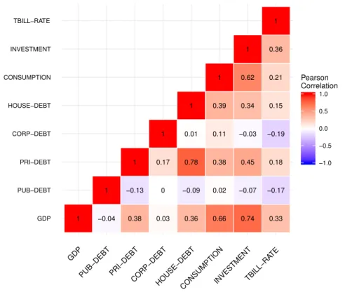
Looking at the cross correlations between the log-differences of the variables of interest (in figure 2.2) we get a first glimpse at the relations among our variables. It is interesting to note how public debt is negatively correlated, even if only slightly, with GDP and with all the other variables apart from consumption, with which pub-lic debt is basically uncorrelated. Private debt instead, which is measured by the total amount of credit to the private non-financial sector, is positively correlated with all the variables. Also when disaggregate into corporate and household debt, this positive correlation still holds true with the unique exception happening in the negative cor-relation between corporate debt and interest rate, which has a theoretical justification for the fact that interest rates measure the cost of borrowing for a firm.
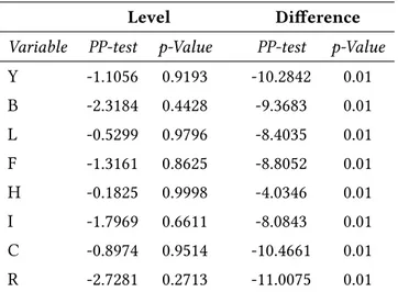
Before performing our time series analysis we look at the integration order of all the variables of interest. We use the Phillips-Perron test which – since it augments the Dickey-Fuller test – is robust also with respect to possible unspecified autocorrelation and heteroskedasticity. The results, presented in table 2.2, do not reject the null hy-pothesis (H0 =“Presence of unit root”) for all the variables in level. On the contrary
the test always rejects the null for all the variables in difference. This suggests that all the variables of interest are integrated of order one – I(1).
1 −0.04 1 0.38 −0.13 1 0.03 0 0.17 1 0.36 −0.09 0.78 0.01 1 0.66 0.02 0.38 0.11 0.39 1 0.74 −0.07 0.45 −0.03 0.34 0.62 1 0.33 −0.17 0.18 −0.19 0.15 0.21 0.36 1 GDP PUB−DEBT PRI−DEBT CORP−DEBT HOUSE−DEBT CONSUMPTION INVESTMENT TBILL−RATE GDP PUB−DEBT PRI−DEBT CORP−DEBT HOUSE−DEBT CONSUMPTIONINVESTMENT TBILL−RA TE −1.0 −0.5 0.0 0.5 1.0 Pearson Correlation
Figure 2.2: Cross correlations of the investigated variables.
2.5 Results
In this section we present the results of the regressions that we have run in order to un-derstand the effects that public and private debt shocks have on the economy. All the regressions here presented are estimated with the variables in level – without differ-entiation or filtering – in order to extract all the information stemming from possible cointegration relations. Table 2.3 reports the variables contained in each regression, the suggested numbers of lags according to the standard criteria and the number of cointegration relations to be included according to the Johansen and Juselius, (1990) procedure.7
7The bold in the lag selection corresponds to our choice. Where possible, we have adopted the
Bayes-Schwartz Criterion (BIC). In the cases in which the adoption of such a criterion was a poor one (because residuals did not display standard properties of a white noise) we have selected the more parsimonious between the Akaike Information Criterion (AIC) and the Hannan–Quinn Criterion (HQ). All the cointegration relations are estimated with a constant. All the estimations, unless clearly specified,
Level Difference Variable PP-test p-Value PP-test p-Value Y -1.1056 0.9193 -10.2842 0.01 B -2.3184 0.4428 -9.3683 0.01 L -0.5299 0.9796 -8.4035 0.01 F -1.3161 0.8625 -8.8052 0.01 H -0.1825 0.9998 -4.0346 0.01 I -1.7969 0.6611 -8.0843 0.01 C -0.8974 0.9514 -10.4661 0.01 R -2.7281 0.2713 -11.0075 0.01
Table 2.2: Phillips-Perron test for stationarity.
ID Variables Lags (p) Cointegration order (r) Period 1 Y, B, L, R AIC: 10, HQ: 6, BIC: 5 1 1966 - 2015 2 Y, B/Y, L/Y, R AIC: 10, HQ: 6, BIC: 5 1 1966 - 2015 3 Y, B, L, I, R AIC: 10, HQ: 6, BIC: 1 2 1966 - 2015 4 Y, B, L, C, R AIC: 6, HQ: 5, BIC: 1 2 1966 - 2015 5 Y, B, F, I, R AIC: 8, HQ: 5, BIC: 2 2 1966 - 2015 6 Y, B, H, C, R AIC: 6, HQ: 4, BIC: 2 1 1966 - 2015
Table 2.3: Regressions settings.
Before proceeding further and discussing about the structural and causal infor-mation that we have extracted from the identification procedure, we here present the estimated cointegration relations in table 2.4. Even if here we are interested in causal, structural properties between the variables, and cointegration is a property of the re-duced form model, it is interesting to observe the estimated cointegration relations in order because they suggest possible long-run relations between our variables of inter-est.
In what follows we describe our results in detail. We first present the results of the baseline models (the regressions with ID numbers 1 and 2), we then proceed by presenting the results of the augmented models (with ID numbers 3 and 4), finally we
Variable ID 1 ID 2 ID 3 (r=2) ID 4 (r=2) ID 5 (r=2) ID 6 Y 1 1 1 0 1 0 1 0 1 B -0.0052 -0.0184 0 1 0 1 0 1 -0.1763 L -0.7092 -2.4835 -3.3690 -21.2617 -0.5813 -22.9709 F -0.3506 -2.1589 H -0.3714 I 3.6784 27.6748 -0.4433 1.7958 C -0.1832 29.1448 -0.1634 R -1.2553 -4.3960 -10.7382 -71.2981 -1.1836 -25.0376 0.3161 2.6357 -1.8142 const. -5.7968 2.7435 1.0895 54.1615 -4.8187 -151.8507 -7.4530 -0.1093 -5.5472
Table 2.4: Estimated cointegration relations (βt).
describe the findings of the disaggregated regressions (the models with ID numbers 5 and 6). We conclude the section by presenting some corollary results which study the crowding-out or crowding-in effects of public debt shocks on private consumption and on private investment and by presenting robustness checks related to the estimation of a model in a subsample without the crisis period.
2.5.1 Baseline models
The baseline regressions we consider here are the two four-dimensional VECMs that are presented in the first two rows of table 2.3. The first model is a very simple specifi-cation that contains GDP, government debt, non-financial firms debt ant the 3-months T-Bill interest rate that allows to control for the effects brought about by monetary pol-icy. The second model employs the same variables, but with public and private debt which are measured as ratios with respect to GDP. This latter specification is included because the measurement of the variable is the closest to the typical panel data esti-mations which attempt at measuring the effects of public Debt-to-GDP on economic growth (see Panizza and Presbitero, 2013, and most of the literature presented in sec-tion 2.2). In spite of their simplicity these two models are able to capture the bulk of the effects that we also find on richer specifications.
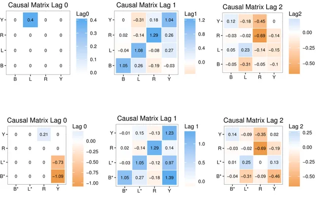
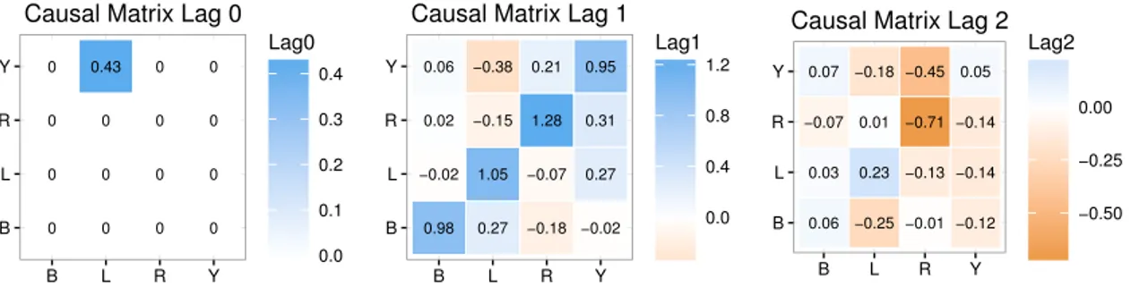
Figure 2.3 contains the matrices of the structural VARS: even if the contemporane-ous causal structure differ between the two models (Lag 0 matrices), the results
stem-ming from the estimation and identification of these models are pretty much similar (Lag 1 and Lag 2 matrices).8 The first two matrices on the left (Lag 0) represents the
matrix B = I − Γ0 – which has been identified with our data-driven causal search
procedure. It is interesting to note that there is quite a difference between the two and this might be due to the fact that the measure of the two debt variables are different; in the second model indeed, GDP also appear in the denominator of the debt variables, creating some additional endogenous relation that our algorithm captures.
0 0 0 0 0 0 0 0 0.4 0 0 0 0 0 0 0 B L R Y B L R Y 0.0 0.1 0.2 0.3 0.4 Lag0
Causal Matrix Lag 0
1.04 −0.03 0.27 0.26 0 1.05 −0.04 0.02 −0.31 0.26 1.08 −0.14 0.18 −0.19 −0.08 1.29 B L R Y B L R Y 0.0 0.4 0.8 1.2 Lag1
Causal Matrix Lag 1
0 −0.1 −0.15 −0.14 0.12 −0.05 0.05 −0.03 −0.18 −0.31 0.23 −0.02 −0.45 −0.05 −0.14 −0.69 B L R Y B L R Y −0.50 −0.25 0.00 Lag2
Causal Matrix Lag 2
0 −1.09 −0.73 0 0 0 0 0 0 0 0 0 0.21 0 0 0 B* L* R Y B* L* R Y −1.00 −0.75 −0.50 −0.25 0.00 Lag 0
Causal Matrix Lag 0
1.23 1.39 0.97 0.14 −0.01 1.05 −0.03 0.02 0.15 0.27 1.05 −0.14 −0.13 −0.18 −0.12 1.29 B* L* R Y B* L* R Y 0.0 0.5 1.0 Lag 1
Causal Matrix Lag 1
0.02 −0.46 0.13 −0.19 0.14 −0.04 0.01 −0.03 −0.09 −0.31 0.25 −0.02 −0.35 −0.09 0 −0.69 B* L* R Y B* L* R Y −0.50 −0.25 0.00 0.25 Lag 2
Causal Matrix Lag 2
Figure 2.3: SVAR causal matrices up to the 2ndlag for the baseline models 1 (top panels)
and 2 (bottom panels). The entry below the table causes the entry on the left of the table.
The two contemporaneous causal structures are also depicted in figure 2.4, in a standard Directed Acyclic Graph (DAG) form. Concerning the first model, the
temporaneous causal structure suggests that output is positively caused by private debt while the other variables does not have contemporaneous impact. The second graph, representing model 2, contains the information entailed in the bottom-left ma-trix in figure 2.3. Identification suggests that interest rate slightly affects output which, in turn, negatively affects both private and public debt to GDP. This difference might be due to the fact that macroeconomic variables are all intrinsically endogenous, and the identification of a causal order that does not allows for loops produces uncertainty in the direction of contemporaneous causality, or also to the fact that the debt variables are measured in different ways in the two models. Notwithstanding the contemporane-ous differences, it has to be noticed, that in both the cases the lagged causal structure is very similar (see figure 2.3) and this is particularly important for dynamic causal consideration. L + Y R Y L∗ B∗ + − −
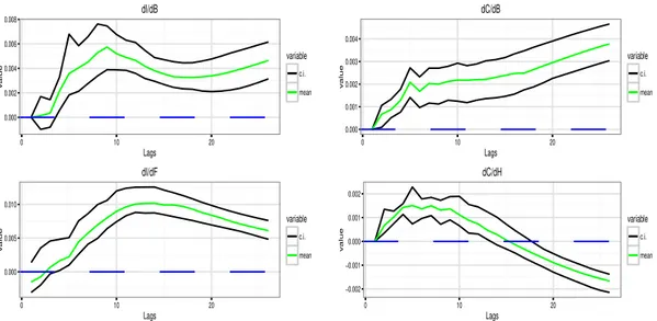
Figure 2.4: Contemporaneous causal structure of models 1 (left) and 2 (right). As we move to dynamic causal considerations, the natural tool that we adopt for estimating the causal effects that a shock to one variable has on the other variables is the “Impulse Response Function” (IRF). The estimated IRF for the two baseline models are depicted in figure 2.5 and are robust also to different model estimation strategy, such as the level-VAR estimated with OLS. The fact that the IRFs do not converge to the zero level is due to the fact that we estimate the model in level, without differentiating the variables, which is consistent with the Johansen, (1995) procedure.9
The results provide a new piece of evidence for what concerns the effects of public debt shocks and corroborate existing evidence presented in section 2.2 for what con-cerns the effects stemming from private debt shocks. As a matter of fact we find that a positive shock to public debt is persistently beneficial for economic growth, causing
9The represented confidence intervals are those calculated by means of bootstrapping techniques at
0.000 0.002 0.004 0.006 0 10 20 Lags v alue variable c.i. mean dY/dB 0.000 0.002 0.004 0 10 20 Lags v alue variable c.i. mean dY/dL 0.000 0.002 0.004 0.006 0 10 20 Lags v alue variable c.i. mean dY/dB −0.003 −0.002 −0.001 0.000 0.001 0.002 0 10 20 Lags v alue variable c.i. mean dY/dL
Figure 2.5: IRF of baseline models 1 (left) and 2 (right).
output to increase. A private debt shock instead, while being beneficial for GDP in the short-run – during the first two and a half years (10 quarters) after the shock hits – has negligible or even negative effects on output on longer horizons. We argue that the statistical significance of a negative effect is brought about by the higher likelihood of financial crisis that a higher private debt brings about, as stated in the series of papers by Jordà et al., (2013, 2014, 2016).
2.5.2 Augmented models
Concerned by the fact that in our two baseline specifications, some omitted variables might mediate and have relevant effects, we also estimate two richer models including possibly mediating features; these are dubbed the augmented models and in table 2.3 have respectively the ID 3 and 4. In both cases, we augment the first baseline model including aggregate investment (in model 3) and aggregate private consumption (in model 4).
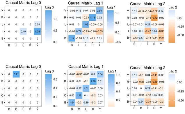
Figure 2.6 represents the matrices of the structural VARs for the models 3 (top row) and 4 (bottom row). Again, the contemporaneous causal structure is different between the two models: this time the difference might be due to the change of variable. Still,
0 0 0.28 1.38 0 0 0 0 0 0 0 0 0 0.49 0 0 0 0 0 0 0 0 0 0 0 B I L R Y B I L R Y 0.0 0.5 1.0 Lag 0
Causal Matrix Lag 0
0.94 0.11 −0.08 −0.59 0.22 −0.02 1.14 0.02 −0.08 0.05 0.07 0.18 1.06 −0.29 −0.23 0.18 −0.09 0 0.71 0.06 0.02 −0.1 −0.09 −0.16 1.18 B I L R Y B I L R Y −0.5 0.0 0.5 1.0 Lag 1
Causal Matrix Lag 1
0.14 −0.37 −0.09 −0.33 −0.02 0.11 −0.13 −0.03 0.06 0.02 −0.14 −0.13 0.22 −0.47 −0.14 −0.14 0.17 0.01 0.1 −0.05 −0.32 −0.14 −0.06 0.24 −0.72 B I L R Y B I L R Y −0.50 −0.25 0.00 Lag 2
Causal Matrix Lag 2
0 0 0 0 0 0 0 0 0 0 0 0 0 0 0 0.71 0 0 0 0 0 0 0 0 0 B C L R Y B C L R Y 0.0 0.2 0.4 0.6 Lag 0
Causal Matrix Lag 0
0.84 0.07 0.08 0.03 0.31 −0.03 1.04 −0.04 0.03 0.02 −0.06 0.29 1.01 0.1 −0.1 −0.33 −0.2 0.27 1.12 0.01 0.3 −0.2 −0.05 −0.2 1.28 B C L R Y B C L R Y 0.0 0.4 0.8 1.2 Lag 1
Causal Matrix Lag 1
0.02 −0.2 −0.1 0.04 −0.05 0.11 −0.04 0.03 −0.01 −0.02 0.04 −0.34 0.22 −0.12 −0.02 −0.1 0.24 0 −0.04 −0.28 −0.41 −0.09 −0.11 0.05 −0.69 B C L R Y B C L R Y −0.50 −0.25 0.00 Lag 2
Causal Matrix Lag 2
Figure 2.6: SVAR causal matrices up to the 2ndlag for the baseline models 1 (top panels)
and 2 (bottom panels). The entry below the table causes the entry on the left of the table.
the lagged components contains pretty much the same effects; moreover, the bulk of these effects is consistent with the two baseline models presented above.
The contemporaneous causal structure is also represented in DAG form in figure 2.7. In model 3 it is possible to observe the double contemporaneous role played by GDP as a booster for both private debt and private investment; private debt also has a positive effect on investment. Concerning model 4 instead, the unique significant contemporaneous causal effect is played by consumption on output.
The dynamic causal relations are represented by means of IRF in figure 2.8. The results confirm, and even reinforce, the claims stemming from the two baseline esti-mations. Public debt shocks do cause higher output while private debt shocks have positive and mild effects in the short-run, but negative effects in the long-run. IRF are
Y L I + + + C Y +
Figure 2.7: Contemporaneous causal structure of models 3 (left) and 4 (right). the typical tools used also for policy analysis and in our models they suggest that pub-lic debt cannot be harmful for the US economic system, but instead might be a good device for restoring economic growth.
0.000 0.001 0.002 0.003 0.004 0.005 0 10 20 Lags v alue variable c.i. mean dY/dB −0.003 −0.002 −0.001 0.000 0.001 0.002 0 10 20 Lags v alue variable c.i. mean dY/dL 0.000 0.001 0.002 0.003 0.004 0 10 20 Lags v alue variable c.i. mean dY/dB −0.004 −0.002 0.000 0 10 20 Lags v alue variable c.i. mean dY/dL
Figure 2.8: IRF of augmented models 3 (left) and 4 (right).
Across the four different specifications presented up to now, the three difference that shall be noticed are with respect to (i) the contemporaneous causal structure, (ii) the size of the effects in the IRFs and (iii) the number of lags after which the private debt begins to affect output negatively in the IRFs. Concerning the first point, we argue that the changes in measurement (level or ratio) and the changes in variables (investment or consumption) might be the motives behind the observed differences. With respect to the second difference, estimations seem to be consistent one with the other between 0.3% and 0.6% for what concerns public debt; for private debt instead, the support varies between a maximum of 0.5% and a minimum of −0.4% reflecting
partly the higher variability of the effect over time and partly the higher variability of the estimation across the four specifications. About the third relevant point of differ-ence instead – i.e. the number of lags for the effects of private debt to change its sign – we note that in the estimations this value lays between a minimum of 10 lags to a maximum of 20 lags in the best case scenario. However, it shall be noticed that in one scenario, the negative effect of private debt does not appear and instead, private debt only becomes insignificant after 20 lags.
2.5.3 Disaggregated models
We then proceed with our analysis by decomposing the total private debt into two smaller components: mortgage and corporate debts. Such a procedure allows us to address the possible issue of having selected a wrong/bad proxy for aggregate private debt – even if the variable that we use as a proxy for private debt is the “total credit to private non-financial sector”, and has been already extensively used in the literature, also in the seminal contribution by Jordà et al., 2014. Moreover, such a decomposition allows us to better understand at a more disaggregated level how debt to different microeconomic entities – namely households for what concerns mortgages and firms for what concerns corporate debt – might differently impact on output.
The causal SVAR matrices for these disaggregated scenarios are presented in figure 2.9 while the implied contemporaneous causal structure is plotted in figure 2.10. Two points are worth to be noticed here. First, the causal structure of the two models are very similar with respect to the augmented models: this is so because we did not had a full change in the measurement or in the variables as we did before, since in both cases, disaggregated private debt remain proxies of the aggregated private debt. Hence it is with no surprise that we observe output causing investment in model 5 – even if here it is interesting to notice that corporate debt plays no role – and consumption causing output in model 6. Second, the fact that the lagged effects are again consistent with all the previous regressions, confirming that the baseline models are able to capture most of the effects.
Again, the dynamic results are presented in figure 2.11 by means of the IRFs. The results suggest that, while the effects of public debt remain positive both in the short
0 0 0 1.47 0 0 0 0 0 0 0 0 0 0 0 0 0 0 0 0 0 0 0 0 0 B F I R Y B F I R Y 0.0 0.5 1.0 Lag 0
Causal Matrix Lag 0
0.86 0.28 −0.05 −0.65 0.11 −0.01 1.11 0.01 −0.07 −0.02 0.04 −0.01 1.21 0.04 −0.1 0.23 −0.19 0.01 0.91 0.08 0.07 −0.15 −0.14 −0.18 1.2 B F I R Y B F I R Y −0.5 0.0 0.5 1.0 Lag 1
Causal Matrix Lag 1
0.11 −0.25 0.31 −0.54 −0.04 0.14 −0.09 0.05 −0.06 0.02 −0.04 0.15 −0.15 −0.04 0.01 −0.15 0.17 −0.01 0 −0.09 −0.32 −0.16 0.23 0.23 −0.62 B F I R Y B F I R Y −0.6 −0.4 −0.2 0.0 0.2 Lag 2
Causal Matrix Lag 2
0 0 0 0 0 0 0 0 0 0 0 0 0 0 0 0.71 0 0 0 0 0 0 0 0 0 B C H R Y B C H R Y 0.0 0.2 0.4 0.6 Lag 0
Causal Matrix Lag 0
0.85 0.18 −0.04 0.02 0.31 −0.07 1.11 0.03 0.03 0.04 −0.05 0.22 1.41 0.23 −0.01 −0.33 −0.41 0.05 1.12 0 0.28 −0.18 −0.08 −0.24 1.25 B C H R Y B C H R Y 0.0 0.5 1.0 Lag 1
Causal Matrix Lag 1
0.04 −0.3 0.09 0.08 −0.08 0.13 −0.09 0.04 0 0.04 0.05 −0.06 −0.37 −0.32 −0.29 −0.18 0.48 0.16 0.06 −0.2 −0.39 −0.18 −0.06 0.13 −0.73 B C H R Y B C H R Y −0.50 −0.25 0.00 0.25 Lag 2
Causal Matrix Lag 2
Figure 2.9: SVAR causal matrices up to the 2ndlag for the baseline models 5 (top panels)
and 6 (bottom panels). The entry below the table causes the entry on the left of the table.
and in the long-run (and converging to a value between 0.3% and 0.6%, consistently with the previously presented estimations), decomposing the private debt into mort-gage and corporate debts allows a better understanding of the origin of the long-term negative effects caused by private debt in the all the previous figures. These new re-sults indeed, which are shown in figure 2.11, suggest that not every form of credit to private entities has the same effect on output: corporate debt indeed (left panel) is mostly beneficial and has effects which are very similar to the public debt ones (also in size, even if in the long run it decreases); mortgage debt is instead the type of debt mostly harmful, which generates positive effect in the short-run, but strong negative effects in the long-run. Mortgage debt hence, we conclude, is the type of debt that also drives the dynamic of aggregate private debt in the previous results.