Discontinuous Galerkin Methods for inviscid low Mach number flows

(1)

Universit`

a degli studi della Calabria

Dipartimento di Ingegneria Meccanica

Tesi di Dottorato di Ricerca

in Ingegneria Meccanica

Discontinuous Galerkin Methods

for inviscid low Mach number flows

Ing. Alessandra Nigro

Supervisore Ing. Carmine De Bartolo

Co-Supervisore Prof. Francesco Bassi

Coordinatore Prof. Maria Laura Luchi

Dr. Ralf Hartmann

Novembre 2007

DOTTORATO DI RICERCA XX Ciclo

(2)

Discontinuous Galerkin Methods

for inviscid low Mach number flows

by

Eng. Alessandra Nigro

Submitted to the Department of Mechanical Engineering on November 23, 2007,

in partial fulfilment of the requirements for the Ph.D. of Mechanical Engineering

Abstract

In this work we present two preconditioning techniques for inviscid low Mach number flows. The space discretization used is a high-order Discontinuous Galerkin finite element method. The time discretizations analyzed are explicit and implicit schemes. The convective physical flux is replaced by a flux differ-ence splitting scheme. Computations were performed on triangular and quad-rangular grids to analyze the influence of the spatial discretization. For the preconditioning of the explicit Euler equations we propose to apply the fully preconditioning approach: a formulation that modifies both the instationary term of the governing equations and the dissipative term of the numerical flux function. For the preconditioning of the implicit Euler equations we propose to apply the flux preconditioning approach: a formulation that modifies only the dissipative term of the numerical flux function. Both these formulations permit to overcome the stiffness of the governing equations and the loss of ac-curacy of the solution that arise when the Mach number tends to zero. Finally, we present a splitting technique, a proper manipulation of the flow variables that permits to minimize the cancellation error that occurs as an accumulation effect of round-off errors as the Mach number tends to zero.

(3)

Chapter 1 Introduction

The use of numerical methods to simulate complex physical phenomena has become an invaluable part of engineering and modern science. Among them, Computational Fluid Dynamics (CFD) has matured significantly in past decad-es, in terms of time and computational resourcdecad-es, even if large aerodynamic simulations of aerospace vehicles are still very expensive.

Almost all discretizations of the compressible Euler and/or Navier-Stokes equations currently used in aerodynamic applications are based on Finite Vol-ume Methods (FVM). The evolution of these methods, including the incorpo-ration of the upwinding mechanisms [1–5] and advances in solution techniques for viscous flows [6–9], have made the simulation of complex problem possi-ble. However, these standard algorithms remain at best second-order accurate, meaning that the error decrease as O(h2_{) as the grid spacing h tends to zero.}

Moreover, while these methods are used heavily in aerospace design today, the time required to obtain realibly accurate solutions has hindered the realization of the full potential of CFD in the design process. In fact, it is unclear if the accuracy of current second-order finite volume methods is sufficient for engi-neering purposes. The results of the two AIAA Drag Prediction Workshop (DPW) [10, 11] suggest that the CFD technology currently in use may not produce sufficiently accurate results on meshes with typical grid sizes that are

(7)

used in an industrial environment.

This problem could be alleviated by the development of high-order CFD algorithms. Traditional finite volume methods rely on extended stencils to achieve high-order accuracy. This may lead to difficulties in achieving stable iterative algorithms and higher-order algorithms on unstructured meshes. In fact, higher order ENO and WENO reconstruction methods on unstructured meshes are not used for industrial applications. To overcome these problems, significant research effort has been devoted to the development of new high-order accurate methods, among them the Discontinuous Galerkin Finite Ele-ment Methods (DGFEM, DG methods for short). It can be observed that the DG methods have experienced a resurgence of interest in multi-various disci-plines of numerical mathematics including compressible flows and aerodynam-ics among many others, and that these methods are now applied to problems which traditionally were solved using the Finite Volume Methods [12]. The reason for this trend can be identified in several advantages of the discon-tinuous Galerkin methods over finite volume methods. In fact, DG methods allow higher order computations on unstructured meshes, they allow consider-able flexibility in the choice of the mesh design including hanging nodes, non-matching grids and hp-refinement and they can easily be parallelized. This potential of DG methods has attracted the attention to explore the benefits of this approach in the low Mach number limit.

Algorithms ”traditionally” used, like Finite Volume Methods, encounter some difficulties to solve low Mach number flows. One of the difficulties con-sists in a degradation of the computational performance: convergence slows down and/or fails and often the numerical accuracy decreases as the Mach number tends to zero [13, 14]. To overcome the lack of numerical accuracy a very high mesh resolution is required with ulterior convergence rate reductions. Therefore the low Mach number flow simulations performed with numerical schemes currently in use are very expensive.

(8)

Another difficulty in computing flows at very low Mach number arises from the increasing of cancellation errors when the Mach number tends to zero. At low Mach number the changes of thermodynamic flow variables become small with respect to their stagnation values. The accuracy of the numerical solution is lost, as the round-off errors in computing the thermodynamic gradients accumulate and result in large cancellation error.

These are problems well-known and widely examined in literature and many different strategies have been studied trying to overcome these diffi-culties. However, most of these publications are devoted to the analysis and application of these strategies to FVM, while, to the knowledge of the author, only few are based on the DG method solving flows in the low Mach number regime [15, 16].

Motivated by the potential of the DG method and by the necessity to obtain converged and accurate solutions for low Mach number flows, this thesis gives at first a clearer understanding of the performance of the DG method in the low Mach number limit and secondly contributes to the development of a higher-order CFD algorithm which is able to overcome the lacks of convergence and accuracy exhibit by the compressible flow algorithms in the incompressible limit.

Remark : We note that the numerical methods described in this thesis have

been implemented and tested based on two separate Discontinuous Galerkin flow solvers: In the flow solver MIGALE of Prof. Bassi [17] based on non-parametric elements and in the DG flow solver PADGE [18] which is based on the deal.II library [19,20] implementing parametric elements. The results which have been obtained on quadrangular elements based on these two codes have been cross-checked and found to be very similar which significantly increased the confidence in the results obtained and the numerical effects encountered. However, most of the numerical results which are finally printed in this thesis have been produced based on the DG flow solver of Prof. Bassi as it – in

(9)

contrast to deal.II – allows the use of both, quadrangular and triangular meshes.

1.1 Motivation

There is an ever-increasing need of computing compressible low Mach number flows or locally incompressible flows. Typical examples of compressible low speed flows can be found in natural convection flows in gas or liquid phase, subsonic combustion in heat engines or burners, heat transfer in heat exchang-ers and othexchang-ers. Additionally, many problems contain some regions with very low Mach numbers while other regions are decidedly compressible. Thus com-pressibility can not be neglected and numerical procedures for the solution of these problems must be capable of simultaneously treating both high and low speed flow regimes. Some examples include rocket motor flows in which the Mach number is zero at the closed end and supersonic at the divergent nozzle exit, high speed flows with large embedded recirculation zones, multi-phase flows in which the Mach number changes drastically through the multi-phase boundaries, and flow over a wing at high angle of attack [21].

However, it is very difficult or impossible to solve low speed flows with a conventional compressible algorithm. Algorithms used for compressible flows, usually denoted as density-based, as the continuity equation rules the time evolutions of density, suffers from slow convergence and lack of accuracy to solve low Mach number flows in which the density is almost constant. To overcome these problems, different approaches such as pressure correction, pseudo-compressibility methods and different preconditioning techniques have been developed. Up to now, most of the research effort devoted to the efficient computation of low speed flows has been concentrated on low-order methods like the FVM.

In this work we investigate the behaviour in the low Mach number limit and the effect of the preconditioning technique using a high-order method like

(10)

the DG method.

1.2 Background

1.2.1 High-Order Methods

With the expression high-order method we refer to the order of accuracy of the method. The order of accuracy of a numerical method is the exponent of the first term in the Taylor series expansion of the difference between the analytical solution and the approximate solution. For efficiency of the method we refer to the time necessary to achieve a prescribed accuracy level. Since there is always a tradeoff between accuracy and computing time of any numerical method, the most desirable methods the efficient ones, i.e. those for which the running time increases slowly as the acceptable error decreases. Higher-order methods are of interest because they have this potential: the potential to provide significant reductions in the time required to obtain accurate solutions.

The first high-order accurate numerical methods were spectral methods [22, 23], where the solution of a differential equation is approximated using a high-order expansion. By choosing the expansion functions properly, an arbi-trarily high-order accuracy can be achieved. However, because of the global nature of the expansion functions, spectral methods are limited to very sim-ple domains with simsim-ple boundary conditions. Motivated by the prospect of obtaining the rapid convergence rates of spectral methods with the greater geometric versatility provided by finite element methods, in the early 1980s the researchers introduced the so called p-type finite element method. In the

p-type finite element method, the grid spacing, h, is fixed, while the

polyno-mial degree, p, is increased to decrease the error. In 1981, Babuska et al. [24] applied this method to elasticity problems. They concluded that based on degrees of freedom, the rate of convergence of the p-type method cannot be slower than that of the h-type and that, in cases with singularities present at

(11)

vertices, the convergence rate of the p-type is twice as fast. Starting from these first studies significant research effort has been aimed at developing high-order accurate methods, among others the Discontinuous Galerkin Finite Element Method.

1.2.2 Discontinuous Galerkin Methods

The Discontinuous Galerkin Method was originally developed by Reed and Hill [25] in 1973 for neutron transport problems and first analyzed by Le Saint and Raviart in 1975. Since that time, development of the method has proceeded rapidly. Cockburn et al. present an extensive overview of the history of DG methods in [26].

The DG methods combine ideas from the finite element and the finite volume methods: the accuracy obtained by high-order polynomial approxi-mations within elements and the physics of wave propagation expressed by Riemann problems. In contrast to standard finite element methods the DG methods are based on discontinuous basis functions. Given a mesh of the computational domain, the DG methods approximate the solution within each element by a function from a low-dimensional vector space of functions, e.g. as a linear combination of basis functions like polynomials. For a pair of adja-cent mesh elements, the approximate solution computed in the interior of the elements does not have to agree on the element interface.

The DG method has several desirable properties that have made it popular:

• It can sharply capture solution discontinuities relative to a computational

mesh.

• It simplifies adaption since inter-element continuity is neither required

for mesh refinement and coarsening, nor for p-adaptivity.

• It conserves the appropriate physical quantities (e.g. mass, momentum

(12)

• It can handle problems in complex geometries to high order.

• Regardless of order, it has a simple communication pattern to elements

sharing a common face that simplifies parallel computation.

On the other hand, with a discontinuous basis, the DG methods include more unknowns for a given order of accuracy on a given mesh than traditional finite element or finite volume methods, which may lead to some inefficiency.

1.2.3 Preconditioning Techniques

It is well-known that convergence and accuracy slow down solving low Mach number flows [14]. The reason of the bad convergence is the large disparity between acoustic and convective wave speeds that causes the ill-conditioning (stiffness problem) of the governing equations. The decreasing accuracy re-sults from a lack of artificial dissipation for small Mach number, as observed in related work carried out by Turkel et al. [27]. In particular, for the upwind schemes Guillard and Viozat [28] show that the dissipative terms of the nu-merical flux become negligible with respect to the centered ones as the Mach number tends to zero. In order to accurately and efficiently solve nearly in-compressible inviscid flows these difficulties must be overcome, which is the goal of the preconditioning techniques.

The preconditioning technique artificially modifies the acoustic wave speeds by modifying the time derivative terms of the governing equations. These pseudo-acoustic wave speeds can be chosen of the same order as the local velocity to drastically reduce the condition number. As a consequence, the convergence of the time-stepping or iterative solution process is significantly enhanced. Furthermore, the accuracy of the discretization can be improved by preconditioning if the numerical dissipation term is modified accordingly. In particular, the preconditioned governing equations preserve the accuracy for nearly incompressible flows. This is obtained by balancing appropriately the artificial viscosity term with the inviscid flux term [27–29]. Some of the

(13)

most recognized local preconditioners for inviscid and viscous flows were pro-posed by Choi and Merkle [30], Turkel [31, 32], Lee and van Leer [33] and Weiss and Smith [34], respectively. As the preconditioning destroys the time accuracy, it is applicable to steady-state simulations, only. To overcome this limitation, dual time-stepping techniques may be employed [34]. Numerous studies have been carried out on these topics in the past; a complete review of the preconditioning techniques is given in [31–33, 35].

1.3 Outline of Thesis

This thesis deals with a high-order accurate discontinuous finite element method for the numerical solution of the compressible Euler equations on triangular and quadrangular unstructured grids in the low Mach number limit.

The outline of this work present Thesis is as follows:

• In Chapter 2 we present the physical model obtained premultiplying the

time derivative of the governing Euler equations by the preconditioned matrix.

• In Chapter 3 we describe the Discontinuous Galerkin discretization of

the preconditioned Euler equations.

• In Chapter 4 we present the fully preconditioning technique employed for

explicit schemes. This technique modifies both the instationary terms of the governing equations and the dissipative terms of the numerical flux.

• In Chapter 5 we present the flux preconditioning technique employed

for implicit schemes. This technique modifies the dissipative terms of the numerical flux, only, while the instationary terms of the governing equations remain unchanged.

(14)

• In Chapter 6 we present a splitting technique to minimize cancellation

errors that occur when computing flows at very low Mach number. Finally, we give a conclusion at the end of this work.

(15)

Chapter 2 Physical model

This chapter is devoted to the introduction of the physical model used to in-vestigate the behaviour of the DG method in the low Mach number limit. After a short description of the well-known conservation laws, we focuse our attention on the compressible Euler equations that describe the pure convec-tion of flow quantities in an inviscid fluid. The Euler equaconvec-tions are commonly written in conservative variables but, since the density is a constant in the incompressible limit, a different choice of set of variables could be more ap-propriate; furthermore, for low Mach number, the system of Euler equations become stiff when marching in time. This chapter is then devoted to explain the reasons that induce to apply the preconditioning techniques and the math-ematical meaning of preconditioned physical model.

(16)

2.1 Conservation Laws

2.1.1 Description

A conservation law is a mathematical statement concerning the conservation of one or more quantities. In physical applications an example might be the statement that mass, momentum and energy should be conserved with respect to a specified control volume. The conservation of these flow quantities means that their total variation inside an arbitrary volume can be expressed as the net effect of the amount of the quantity being transported across the boundary, any internal forces and sources, and external forces acting on the volume. In two space dimensions a system of conservation laws is given by

∂ ∂tw (x, t) + ∂ ∂x1 f (w (x, t)) + ∂ ∂x2 g (w (x, t)) = 0, (2.1) where x = (x1, x2)T ∈ R2, w : R2 × R → Rm is an m-dimensional vector

of conserved quantities, or state variables and f (w) and g (w) : Rm _{→ R}m

are the convective flux functions for the system of conservation laws. The equation (2.1) must be augmented by some initial conditions and also possibly boundary conditions on a bounded spatial domain. The simplest problem is the pure initial value problem, or Cauchy problem, in which (2.1) holds for

−∞ < x < ∞ and t ≥ 0.

In this case we must specify initial conditions only

w (x, 0) = w0(x) − ∞ < x < ∞

For brevity, partial derivatives will be denoted by subscripts in the following, and the flux functions will be grouped in the flux vector F = F (f, g). Using this notation, equation (2.1) is given by

wt+ ∇ · F = 0.

The conservation laws considered in this work are the compressible Euler equations that constitute an hyperbolic system of partial differential equations.

(17)

We assume that the System (2.1) is hyperbolic if any real combination of

αf0_{+ βg}0 _{of the flux Jacobians is diagonalizable with real eigenvalues.}

2.1.2 The compressible Euler equations

The compressible Euler equations describe the pure convection of flow quan-tities in an inviscid fluid. In two space dimension they are given in strong and conservative form as follows

wt+ ∇ · F = 0, (2.2)

where w is the state vector of conservative variables given by w =

³

ρ, ρu, ρv, ρE

´_T

,

and F = F (f, g) is the inviscid flux vector, with the inviscid flux functions

f =         ρu ρu2 _{+ p} ρuv ρuH         , g =         ρv ρvu ρv2_{+ p} ρvH         .

Here, ρ is the fluid density, u and v are velocity components, p is the pres-sure and E is the total internal energy per unit mass. The total enthalpy per unit mass, H, is given by H = E + p/ρ, and, assuming the fluid sat-isfies the equation of state of a perfect gas, the pressure is given by p = (γ − 1) ρ [E − (u2_{+ v}2_{) /2], where γ is the ratio of specific heats of the fluid,}

given by γ = cp/cv.

The conservative variables are commonly used in compressible flow compu-tations. Nevertheless, as the Mach number tends to zero, the density becomes constant and cannot be used as a variable in the incompressible limit. Thereby, the set of conservative variables cannot be employed for these flow conditions. A different set of variables may be used, but it must be carefully chosen as each set posses unique properties that influence the performance of the numerical scheme [36].

(18)

The advantage of the primitive variables over other sets is that they are more appropriate for incompressible flow. Since the density is a constant in the incompressible limit, the choice of pressure p as a fundamental variable proved to be more adequate. Moreover, for viscous flows, temperature gradients have to be computed for the thermal diffusion terms, so it also more convenient to work with temperature.

For these reasons, the choice of primitive variables is a ”natural” choice. Furthermore, in [36] it has been shown that the conservative incompressible formulation is well defined only for entropy variables and primitive variables including pressure. It is also shown that these two sets of variables possess the most attributes for practical problem solving, with the primitive variables be-ing more accurate than the entropy variables for low speed and incompressible flows computations. For these reasons the primitive variables are often pre-ferred to perform low Mach number flow computations and they can be used to derive numerical schemes that are suitable for compressible and incompressible flows.

For these reasons, the starting point to obtain compressible Euler equa-tions that are more adequate for the low Mach number limit, is to transform Equations (2.2) in terms of primitive variables, obtaining

Γqt+ ∇ · F = 0.

Here, q is the set of primitive variables given by

q = ³

p, u, v, T

´_T

,

and Γ is the transformation matrix from conservative to primitive variables

Γ = ∂w ∂q =         ρp 0 0 ρT ρpu ρ 0 ρTu ρpv 0 ρ ρTv ρpH − 1 ρu ρv ρTH + ρcp         ,

(19)

where ρp and ρT are given by ρp= ∂ρ ∂p ¯ ¯ ¯ ¯ T =const. , ρT= ∂ρ ∂T ¯ ¯ ¯ ¯ p=const. .

For an ideal gas we have

ρp = 1/T , ρT = −ρ/T .

2.2 The preconditioned compressible Euler

equa-tions

For low Mach numbers the system of Equations (2.2) becomes stiff. The stiffness of the governing equations, when marching in time, is determined by the condition number. The condition number of a general matrix A based on the Lp norm is

Kp(A) = ||A||p||A−1||p.

For the 2D Euler equations, the respective matrices to be considered are linear combinations of the flux Jacobians which have a complete set of eigenvalues and eigenvectors. Thereby we have

K2(A) =

|λ|max

|λ|min

,

where |λ|max and |λ|min are largest and smallest absolute wave speeds. The

wave speeds of the 2D Euler equations are (un, un, un+ c, un− c) where un =

v · n is the component of the velocity vector v = (u, v)T along the unit normal n, also called contravariant velocity, and c is the acoustic velocity (speed of sound).

Thereby, the condition number is given by

K2(A) =

|un| + c

|un|

. (2.3)

In order to explain why the characteristic condition number determines the stiffness of the system of equations when marching in time, we have to recall the

(20)

concept of explicit local time-stepping. The local time-stepping must satisfy the CFL condition: ∆t 6 h |λ|max 6 h |un| + c ,

where h is some representative mesh width. We see, that the allowable local time step is limited by the fastest moving wave |un| + c but we also see that

during such a time step the slowest wave moves only over a fraction of the cell width: |λ|min∆t 6 |λ|min |λ|max h 6 h K2(A) .

Thus a large condition number reduces the efficiency of wave propagation, needed for convergence.

Figure (2.1) shows the condition number for different flow regimes, indicat-ing that the stiffness of the original Euler equations increases beyond bound as the Mach number approaches 0 or 1. This implies that, in order to reduce the stiffness, preconditioning should focus on the incompressible and transonic flow regions.

Figure 2.1: Condition Number

The central idea of preconditioning is the pre-multiplication of the un-steady terms in Equations (2.2) with a matrix, which changes the eigenvalues such that they get closer together. Altering the speed of the un+ c and un− c

waves such that they are comparable with the unwaves, the condition number

(21)

is obtained in much fewer iterations or time steps. Unfortunately the introduc-tion of the precondiintroduc-tioning matrix leads to a formulaintroduc-tion that is not consistent in time and thus is applicable to steady flows, only. To overcome this limita-tion, dual time-stepping techniques may be employed.

The preconditioning technique consists of replacing Γ by another matrix ¯Γ, which we leave unspecified at the moment. The preconditioned Euler equa-tions, still in terms of primitive variables, are then given by

¯

Γqt+ ∇ · F = 0.

2.3 Non-dimensionalization

Mathematical problem formulations based on dimensional and non-dimensionalized variables are essentially equivalent and do not per se alter their solutions. Since the Euler equations are homogeneous, it is preferable to solve them in a non-dimensionalized form. These results can then be applied to any problem with the same relative geometric dimensions. Furthermore, non-dimensionalized variables can be used to extract useful information about relative scales in equations and/or boundary conditions that can guide the preconditioned for-mulation. For these reasons, the following reference values denoted by a sub-script r are used: length lr, density ρr, pressure pr. constant gas Rr.

Reference values for the other quantities are derived from these by functional relationships.

With this choice of non-dimensionalized variables, all the equations given previously remain unchanged, except that the variables are now understood to be non-dimensionalized.

(22)

Chapter 3 Discontinuous Galerkin

Formulation

In this chapter we introduce a high-order accurate discretization of the com-pressible Euler equations. The formulation given in this chapter is valid for both versions of the conservative system equations considered in this work: the standard and the preconditioned Euler equations, both expressed in terms of primitive variables. The introduction of the preconditioned matrix modifies the characteristics of the system equations. As a consequence the precondi-tioned system needs different formulations of the numerical flux and of the boundary conditions, which both are discussed in this chapter. In particu-lar, we perform an analysis on the numerical accuracy of the standard and preconditioned Roe’s approximate Riemann solver in the low Mach number limit.

(23)

3.1 Discretization of the Euler equations

The preconditioned Euler equations in strong and conservative form are given by

¯

Γqt+ ∇ · F = 0, (3.1)

where ¯Γ represent the preconditioned matrix. In absence of preconditioning ¯

Γ reduces to the transformation matrix Γ from conservative to primitive vari-ables and the discretization given below refers to the non-preconditioned Euler equations expressed in terms of primitive variables.

Multiplying Equations (3.1) by a vector-valued test function v and inte-grating by parts, we obtain the weak formulation:

Z Ω vTΓq¯ tdx − Z Ω ∇vT · Fdx + Z ∂Ω vTF · nds = 0 ∀v ∈ H1(Ω) where Ω is the domain, ∂Ω is its boundary, and n is the outward pointing unit normal. To discretize in space, we define V_hp to be the space of discontinuous vector-valued polynomials of degree p on a subdivision Th of the domain into

non-overlapping elements such that Ω =S_k∈T_hκ. Thus, the solution and test

function space is defined by

V_hp =©v ∈ L2(Ω) : v |κ∈ Pp, ∀κ ∈ Th

ª

,

where Pp _{is the space of polynomial functions of degree at most p. The discrete}

problem then takes the following form: find q_h ∈ V_hp such that X κ²Th ½Z κ vT hΓ (q¯ h)tdx − Z κ ∇vT h · Fdx + Z ∂κ\∂Ω v+T h Hi ¡ q+ h, q−h, n ¢ ds + Z ∂κ∩∂Ω v+T h Hb ¡ q+ h, qbh, n ¢ ds ¾ = 0 (3.2)

for all vh ∈ V_hp, where Hi

¡ q+_h, q−_h, n¢ and Hb ¡ q+_h, qb h, n ¢

are numerical flux functions defined on interior and boundary faces, respectively.

(24)

In this work the Roe-averaged flux is used for the inviscid numerical flux. This flux difference splitting scheme is based on the characteristics of the governing equations. This means that two different formulations of the Roe-averaged flux have to be used:

• The standard Roe numerical flux for the non-preconditioned system.

In this case the transformation matrix Γ doesn’t change the character-istics of the system of equations.

• The preconditioned Roe numerical flux for the preconditioned system.

In this case the preconditioned matrix ¯Γ is introduced in order to change the characteristics of the governing equations in such a manner that they get closer together. This means that to be compatible with the preconditioned system, the flux difference splitting scheme is adapted according to the new characteristic values.

The boundary conditions are imposed weakly by constructing an exterior boundary state, qb

h, which is a function of the interior state and known

bound-ary data. In this work wall and far-field boundbound-ary conditions are used. The far-field boundary conditions are based on the characteristic variables. This means that, like for the numerical flux, two different formulations of the far-field boundary conditions have to be used:

• The standard far-field boundary conditions for the non-preconditioned

system.

• The preconditioned far-field boundary conditions for the preconditioned

(25)

3.2 Numerical Flux function

3.2.1 Roe-average numerical flux

The numerical flux functions used on interior and boundary faces in Equation (3.2) could be any kind of upwind numerical flux. Since the fluxes are normal to the element interface and discontinuities are allowed across the interface, a local Riemann problem can be solved based on the interior and the exterior states q+

h and q−h. Therefore, like in Finite Volume methods, various Riemann

solver can be used to compute the numerical flux.

In this work we employ the Roe’s approximate Riemann solver. This is a linearised solver which means that the governing equations of the Riemann problem have been approximated. Obviously this implies that the solution of the Riemann problem will not be exact anymore, but Roe’s approach has shown that despite the approximations good results can be obtained.

In order to clarify how the numerical flux is modified for the preconditioned system to preserve the accuracy of the solution in the low Mach number limit, we begin by introducing the standard Roe’s approximate Riemann solver that is the one used for the non-preconditioned simulations,

H¡w+, w−, n¢= 1 2

³¡

F++ F−¢− ˜F¡w+, w−¢´· n (3.3) where F+ _{and F}− _{are fluxes computed using the solution vectors w}+ _and

w− _{on each (the interior and the exterior) side of the face, ˜}_{F = |A|∆w, and}

∆w = w−_{− w}+_.

The matrix | ˜A| denotes the so-called Roe matrix or dissipation matrix and is equal to the Jacobian ∂F/∂w. The symbol ˜ denotes that the matrix is calculated using the so-called Roe-averaged variables (see Appendix B for details). The dissipation matrix | ˜A| is defined by

| ˜A| = ˜T| ˜Λ| ˜T−1

(26)

using Roe’s averaging, as well as the matrix of left, ˜T−1_{, and right, ˜}_T,

eigen-vectors, remembering that ˜T is the modal matrix that diagonalizes the matrix ˜

A.

For the preconditioned system we change the eigenvalues and the eigenvec-tors of the system used in the definition of | ˜A|. For this reason we rewrite the second term on the right hand side of Equation (3.3), the so-called dissipation term | ˜A|∆w of the Roe’s numerical flux, using following relation

˜ A∆w =¯Γ¯Γ−1∂F ∂w∆w =¯Γ µ ¯ Γ−1∂F ∂q ¶ ∆q =¯Γ ˜A_Γ¯∆q

where ∆q = q−_{− q}+_{. Thus, ∆w is replaced by ∆q, and ˜}_{A by ¯}_{Γ ˜}_A_¯

Γ, where

˜

A¯_Γ is defined in terms of the preconditioned eigenvalues and eigenvectors by

˜

A_Γ¯ = ˜T¯_ΓΛ˜_Γ¯T˜−1_Γ_¯ .

Here the subscript ¯Γ denotes that the diagonal matrix of eigenvalues and the modal matrix are derived from the preconditioned system, where ˜Λ_Γ¯ is the

diagonal matrix of the preconditioned eigenvalues, and ˜T_Γ¯ diagonalizes the

matrix ¡Γ¯−1_∂F/∂q¢_{. Similarly we replace | ˜}_{A|∆w by ¯}_{Γ| ˜}_A_¯

Γ|∆q.

3.2.2 Low Mach behaviour

In this section we want to analyse the behaviour of the standard and the preconditioned flux difference splitting approximation in the low Mach number limit.

For clarity, here we report the Roe’s numerical flux formulation in the case of the non-preconditioned and the preconditioned scheme:

• Roe non-preconditioned

H (w+_{, w}−_{, n) =} 1

2 ³

(27)

• Roe preconditioned H (q+_{, q}−_{, n) =} 1 2 ³ (F+_{+ F}−_{) − ˜}_F ¯ Γ(q+, q−) ´ · n

As seen in the previous subsection, the dissipation term of the Roe precondi-tioned ˜F_Γ¯ is computed as

¯

Γ ˜T_Γ¯| ˜Λ_Γ¯| ˜T−1_Γ_¯ ∆q. (3.4)

For brevity the analysis is performed for the one-dimensional case; the exten-sion to the multi-dimenexten-sional case is immediate.

The preconditioned matrix ¯Γ used in the present work is the local precondi-tioning matrix of Weiss and Smith [34] written in the one-dimensional case as follows ¯ Γ =      Θ 0 ρT Θu ρ ρTu ΘH − 1 ρv ρTH + ρcp     , where Θ is given by Θ= µ 1 U2 r − ρT ρcp ¶ = µ 1 U2 r + 1 T cp ¶ . (3.5)

Here, Ur is a reference velocity and, for an ideal gas, is defined as

Ur=          εc if |v| < εc, |v| if εc < |v| < c, c if |v| > c, (3.6)

where c is the acoustic speed and ε is a small number included to prevent singularities at stagnation points.

The resulting eigenvalues of the preconditioned one-dimensional Euler equa-tions are given by

λ µ ¯ Γ−1∂F ∂q ¶ = (λ1, λ2, λ3)T = (un, u0n+ c0, u0n− c0)T ,

(28)

where u0 n = un(1 − α), c0 ₌p_α2_u2 n+ Ur2, α = 1 − βUr2 2 , (3.7) β = µ ρp+ ρT ρcp ¶ .

Then, the matrices ˜Λ_Γ¯, ˜T_Γ¯, and ˜T−1_Γ_¯ used in (3.4) are given by

˜ Λ_Γ¯ =      λ1 0 0 0 λ2 0 0 0 λ3     , ˜ T_Γ¯ =      U2 r cpT 0 − ρU2 r T r t ρU2 r t 0 −s t − ρU2 r t 0     , T˜ −1 ¯ Γ =      0 1 1 0 − s ρU2 r − r ρU2 r T ρU2 r 1 ρcp 1 ρcp     , (3.8) where r = λ2− λ1, s = λ3− λ1, t = λ2− λ3.

For the non-preconditioned system ˜T_Γ¯ and ˜T−1_¯_Γ reduce to the left and right

eigenvector matrices in primitive variables, respectively. Using (3.8) we obtain the entries of the preconditioned dissipation matrix ¯Γ ˜T_Γ¯ | ˜Λ¯_Γ| ˜T−1_Γ_¯ as follows

dΓ11 = |λ1| cpT + c1, dΓ12= ρc2, dΓ13= −ρ |λ1| T , dΓ21 = un|λ1| cpT + c3, dΓ22= ρc4, dΓ23= − ρun|λ1| T , dΓ31 = u 2 n|λ1| c T + c5, dΓ32= ρc6, dΓ33= − ρu2 n|λ1| T , (3.9)

(29)

where c1 = |λ2| r − |λ3| s tU2 r , c2 = |λ2| − |λ3| t , c3 = |λ2| r (un− s) − |λ3| s (un− r) tU2 r , c4 = |λ2| (un− r) − |λ3| (un− s) t , c5 = |λ2| r (H − uns) − |λ3| s (H − unr) tU2 r , c6 = |λ2| (H − uns) − |λ3| (H − unr) t .

If the absolute values are computed by assuming that |λ1| = λ1, |λ2| = λ2,

|λ3| = −λ3 and the quantities r, s, t and the eigenvalues (λ1, λ2, λ3) are

writ-ten in terms of u0

n, α, c0 and Ur, see Equations (3.6) and (3.7), we obtain

c1 = c 02_{− u}2 n(1 − α)α c0_U2 r , c2 = un(1 − α) c0 , c3 = unc02(2 − α) − u2nα(1 − α2) c0_U2 r , c4 = c 02_{+ u}2 n(1 − α2) c0 , (3.10) c5 = c02_{[H + u}2 n(1 − α)] − u2nα(1 − α) (H + u2nα) c0_U2 r , c6 = unc02+ un(1 − α) (H + u2nα) c0 .

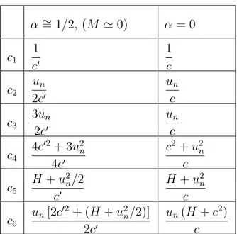
At low Mach number we have α ∼= 1/2, u0n± c0 = 1/2un

¡

1 ±√5¢ and resulting terms are summarized in Table 3.1. In the second column of this table the terms of Equations (3.10) are given in absence of preconditioning (α = 0, u0

n= un, c0 = c = Ur) . We thus obtain the corresponding terms of the

Roe non-preconditioned dissipation matrix, Γ |Γ−1_{∂F/∂q| , where Γ is the}

(30)

α ∼= 1/2, (M ' 0) α = 0 c1 1 c0 1 c c2 un 2c0 un c c3 3un 2c0 un c c4 4c02_{+ 3u}2 n 4c0 c2_{+ u}2 n c c5 H + u2 n/2 c0 H + u2 n c c6 un[2c02+ (H + u2n/2)] 2c0 un(H + c2) c

Table 3.1: Terms occuring in the dissipation matrix of the preconditioned Roe scheme at low speed (first column) and in the dissipation matrix of the non-preconditioned Roe scheme (second column).

Table 3.2 presents the order of magnitude of variables occuring in the pre-conditioned dissipation matrix, ¯Γ¯¯¯Γ−1_∂F/∂q¯¯, and in the non-preconditioned

dissipation matrix Γ |Γ−1_∂F/∂q|.

λ1, un λ2, λ3, r, s, t, Ur H, ρ, T, c

O(M) O(M) if α 6= 0 O(1) O(1) if α = 0

Table 3.2: Order of magnitude of variables occuring in the dissipation matrices.

We now substitute the terms of Table 3.1 in Equations (3.9), use the order of magnitude of the variables given in Table 3.2, and simplify by neglecting all terms except of the lowest-order terms in M .

(31)

For the non-preconditioned Roe scheme at low Mach number (α = 0, M ' 0) we obtain Γ¯¯Γ−1_∂F/∂q¯_{¯ =}          1 c ρ un c −ρ un T un c ρc −ρ u2 n T H c ρun(H + c2) c −ρ u3 n 2T          =     

O(1) O(M) O(M) O(M) O(1) O(M2₎

O(1) O(M) O(M3₎

    .

For the preconditioned Roe scheme at low Mach number (α ∼= 1/2, M ' 0) we obtain ¯ Γ¯¯¯Γ−1∂F/∂q¯¯ =            2 un √ 5 ρ √ 5 −ρ un T 3 √ 5 4ρu_√ n 5 −ρ u2 n T 2H un √ 5 ρH √ 5 −ρ u3 n 2T            =     

O(M−1₎ _O(1) _O(M)

O(1) O(M) O(M2₎

O(M−1₎ _O(1) _O(M3₎

    .

The order of magnitude of the variation of all thermodynamic variables is

O(M2_{), whereas the order of magnitude of the variation of the flow velocity}

is O(M). Thus ∆q = (∆p, ∆u, ∆T )T = (O(M2_{), O(M), O(M}2₎₎T _{. Now we}

multiply the preconditioned and standard Roe dissipation matrices by ∆q, to obtain the corresponding dissipation vectors to compare with the centred terms of the Roe’s approximate Riemann solver. For the non-preconditioned Roe scheme in the low Mach number limit we obtain

Γ |Γ−1_{∂F/∂q| ∆q =}     

O(1) O(M) O(M) O(M) O(1) O(M2₎

O(1) O(M) O(M3₎

          O(M2₎ O(M) O(M2₎      =      O(M2₎ O(M) O(M2₎     . (3.11)

(32)

Considering that the order of magnitude of the centred terms in the Roe approximation are 1 2(F +_{+ F}−_{) =}      O(M) O(1) + O(M2₎ O(M)     , (3.12)

it is evident that the dissipative terms of the non-preconditioned Roe scheme do not scale properly with the convective terms. In particular the comparison of the centred, Equation (3.12), and dissipative terms, Equation (3.11), of the non-preconditioned Roe scheme in the low Mach number limit shows that there is a lack of numerical dissipation of order of O(M−1_{) in the continuity}

and energy equations, whereas an excess of numerical viscosity, of order of

O(M−1_{), results in the momentum equations.}

On the contrary for the preconditioned Roe scheme in the limit of low Mach number we obtain

¯ Γ¯¯¯Γ−1_∂F/∂q¯¯ ∆q =     

O(M−1₎ _O(1) _O(M)

O(1) O(M) O(M2₎

O(M−1₎ _O(1) _O(M3₎

          O(M2₎ O(M) O(M2₎      =      O(M) O(M2₎ O(M)     . (3.13)

Therefore the dissipative terms of the preconditioned Roe scheme in (3.13) scale properly with the convective terms in (3.12). In fact, the precondition-ing increases the numerical dissipation term associated to the continuity and energy equations by a factor of 1/M [28], but reduces the numerical viscosity associated to the momentum equation by a factor of M.

(33)

3.3 Boundary Treatment

3.3.1 Boundary Conditions

Numerical flow simulations consider only a certain part of the physical do-main. The truncation of the computational domain creates artificial bound-aries, where values of the physical quantities have to be specified. Furthermore, walls which are exposed to the flow represent natural boundaries of the physi-cal domain. The correct imposition of boundary conditions is a crucial part of every flow solver. Furthermore, subsonic flow problems are particular sensitive to the boundary conditions. An inadequate imposition can lead to a signif-icant slow down of convergence to the steady state and the accuracy of the solution may be negatively influenced. In particular, the far-field boundary conditions have proven to be decisive for the accuracy and the convergence of steady flows at low Mach numbers. In fact, if the fast acoustic waves may be reflected at a boundary, very quickly corrupting the interior flow field and thereby impairing accuracy and convergence, respectively. Various method-ologies were developed which are capable of absorbing the outgoing waves at the artificial boundary [37, 38]. A review of different non-reflecting boundary conditions can be found in [39, 40].

In this work we consider the following types of boundary conditions:

• Far-field

The numerical imposition of the far-field boundary conditions has to fulfil two basic requirements:

– The truncation of the domain should have no notable effects on the flow solution as compared to the infinite domain.

– Any outgoing disturbances must not be reflected back in to the flowfield.

The far-field boundary conditions are based on characteristic variables. Thus, at inflow the incoming variables that correspond to negative

(34)

eigen-values are specified, and the outgoing variables that correspond to posi-tive eigenvalues are extrapolated.

The standard far-field used in this work for the non-preconditioned sys-tem follow the approach of Whitfield and Janus [41]. This approach is based on the characteristic form of the one-dimensional Euler eqations normal to the boundary.

We note that for the preconditioned system the characteristics of the system are changed although the signs of the eigenvalues remain un-changed. Hence also the far-field boundary conditions must be modified for the preconditioned system.

• Slip wall

In the case of inviscid flows, the fluid slips over the surface. Since there is no friction force, the velocity vector must be tangential to the surface. This is equivalent to the condition that there is no flow normal to the surface, i.e.,

v · n = 0 at slip wall boundaries,

where n denotes the outward unit normal vector at each integration point.

This boundary condition is not based on the characteristics and thus can be employed without change for both systems of equations, the standard and the preconditioned one.

3.3.2 Geometry Representation: Curved Boundaries

As shown by Bassi and Rebay [42], high-order DG methods are highly sensitive to the geometry representation. Thus it is necessary to build a higher-order representation of the domain boundary. In this work, the geometry is repre-sented using a nodal Lagrange basis. Thus the mapping between the canonical

(35)

triangle or square and the element in physical space is given by

x = X

j

x(j)φj(ξ) , (3.14)

where φj is the jth basis function, ξ is the location in the reference space, and

x(j) _{is the location of the jth node in physical space. In general, the}

Jaco-bian of this mapping is not constant, meaning that triangles and quadrangles with curved edges are allowed. Thus by placing the non-interior, higher-order nodes on the real domain boundary, a higher order geometry representation is achieved.

(36)

Chapter 4 Explicit scheme:

Fully Preconditioning technique

for the Euler equations

In this section we discuss implementational issues and numerical results con-cerning the DG method for both the standard and the preconditioned version of the explicit scheme. For the preconditioned explicit scheme, we propose to apply the Fully Preconditioning approach: a formulation that modifies both the instationary terms and the dissipative terms of the numerical convective fluxes. This formulation permits to overcome both the stiffness of the equa-tions and the loss of accuracy of the solution that arises when the Mach num-ber tends to zero. On the other hand, it is not consistent in time and thus applicable to steady flows only.

(37)

4.1 Preconditioning matrix

In the explicit schemes the preconditioning matrix ¯Γ is introduced in the com-pressible Euler equations in order to overcome the stiffness problem that pro-duces serious time-stepping restrictions. The stiffness problem, that we have already see in Section 2.2, is determined by the condition number and is due to the large discrepancy between the speed of sound and the fluid velocity. For clarity here we recall the preconditioned Euler equations,

¯ Γqt+ ∇ · F = 0 (4.1) where F = (f,g) and q =         p u v T         , f =         ρu ρu2_{+ p} ρuv ρuH         , g =         ρv ρvu ρv2_{+ p} ρvH         ,

the transformation matrix from conservative to primitive variables Γ and the preconditioned matrix ¯Γ [34], respectively given by:

Γ =         ρp 0 0 ρT ρpu ρ 0 ρTu ρpv 0 ρ ρTv ρpH − 1 ρu ρv ρTH + ρcp         , ¯Γ =         θ 0 0 ρT θu ρ 0 ρTu θv 0 ρ ρTv θH − 1 ρu ρv ρTH + ρcp         . (4.2) Comparing the transformation matrix Γ with the preconditioned matrix ¯Γ, we notice that the only difference between these two matrices is due to the substitution of ρp by the θ parameter. The term ρpthat multiplies the pressure

time derivative in the continuity equation controls the speed of propagation of acoustic waves in the system. It is interesting to note that, for an ideal gas,

ρp = 1/RT = γ/c2, whereas for constant density flows ρp = 0, consistent with

(38)

Thus, if we replace this term with one proportional to the inverse of the local velocity squared, we can control the eigenvalues of the system such that they are all of the same order. Keeping this in mind, we now proceed to analyse the choice of the θ parameter given by:

θ = µ 1 U2 r − ρT ρcp ¶ .

Here Ur is a reference velocity defined for an ideal gas as follows:

Ur=          εc if |v| < εc, |v| if εc < |v| < c, c if |v| > c, (4.3)

where ε is a small number included to prevent singularities at stagnation points. We choose ε = O (M) to ensure that the convective and acoustic wave speeds are of a similar magnitude, proportional to the flow speed [27]. The resulting eigenvalues of the preconditioned system (4.1) are given by

λ = (un, un, u0n+ c0, u0n− c0) T_, where u0 n = un(1 − α), c0 ₌p_α2_u2 n+ Ur2, α = 1 − βUr2 2 , (4.4) β = µ ρp+ ρT ρcp ¶ .

For an ideal gas β = 1/c2_.

We note that choosing the Urparameter like in Equation (4.3), the

precon-ditioned system is able to switch automatically from the preconprecon-ditioned system to the non-preconditioned one. At low speed we have Ur → 0, α → 1/2, and

all the eigenvalues are of the same order as un.

(39)

c0 _{= c, and ¯}_{Γ reduces to the transformation matrix Γ between conservative}

and primitive variables. In this case Equation (4.1) reduces to the conservative formulation of the non-preconditioned Euler equations in terms of primitive variables.

4.2 Time discretization scheme

In this work we employ an explicit Runge-Kutta time discretization scheme. In Runge-Kutta schemes the solution is advanced in several stages [43] and the residual is evaluated at intermediate states. Coefficients are used to weight the residual at each stage. The coefficients can be optimized in order to expand the stability region and to improve the damping properties of the scheme and hence its convergence and robustness [43–45].

The Kutta scheme employed in this work is a s-stage SSP Runge-Kutta scheme. The solution of the preconditioned system is advanced from time t to time t + ∆t applying the following expression:

q0 _{= q}t_, qi ₌ i−1 X k=0 αikqk+ βik∆t ¡_¯ ΓM¢−1R¡qk¢_, _{i = 1, 2, ..., s,} _(4.5) qt+∆t _{= q}s_,

where i is the stage counter for the s-stage scheme and αik and βik, k =

0, 1, ..., i − 1, are the multistage coefficients for the ith-stage, i = 1, 2, ..., s.

4.3 Local time stepping

The main disadvantage of explicit schemes is that the time step ∆t is severely restricted by the so-called Courant-Friederichs-Lewy (CFL) condition [46]. On the other hand if we are interested in the steady-state solutions only, several

(40)

convergence acceleration methodologies are known in literature. A very com-mon technique is the so-called local time-stepping. The basic idea is to advance solutions in the temporal dimension using the maximum permissible time step for each cell. As a result, the convergence to the steady state is considerably accelerated, but the transient solution is no longer temporally accurate. We have to consider that the preconditioned Euler equations are not consistent in time so, for the preconditioned scheme the local time step ∆t on each element

κ is computed by considering the CF L stability condition:

∆t = CF L · Ωκ Λx

c + Λyc

,

where the preconditioned convective spectral radii are defined as

Λx c = (|¯u0E| + ¯c0x) ∆Sx , Λy c = ¡ |¯v0 E| + ¯c0y ¢ ∆Sy_.

The variables ∆Sx _{and ∆S}y _{represent the projections of the elemental volume,}

Ωκ, on the x and y axis, respectively, whereas ¯u0E, ¯cx0 and ¯vE0 , ¯c0y are obtained

applying Equations (4.4) along the x and y directions and using the mean values of the flow quantities on each element κ.

4.4 Preconditioned Roe’s Numerical Flux

The dissipation part of the preconditioned flux splitting scheme has been im-plemented in the following form:

¯ Γ| ˜A_Γ¯|∆q = |un|         ∆ (ρ) ∆ (ρu) ∆ (ρv) ∆ (ρE)         n + δun         ρ ρu ρv ρH         n + δp         0 i j v         , (4.6)

(41)

where

δun= M∗∆un+ [c∗− (1 − 2α) |un| − αunM∗] ∆p

ρU2 r , δp = M∗_{∆p + [c}∗_{− |u} n| + αunM∗] ρ∆un, ∆un= ∆v · n, c∗ ₌ |u0n+ c0| + |u0n− c0| 2 , M∗ ₌ |u0n+ c0| − |u0n− c0| 2c0 ,

For the non preconditioned system (α = 0, u0

n= un, c0 = Ur = c) this reduces

to the standard Roe’s flux difference splitting when Roe-averaged values are used.

It is interesting to note that when the splitting is written in this form, rather than in the more common form factored in terms of un, |un+ c| and

|un−c| the physical significance of the various added dissipation terms becomes

clear. The three terms in (4.6) represent the interpolation to the cell face of the convected variables, the flux velocity and the pressure, respectively. The first term |un| has the effect of up-winding the convected variables. The second

term δun is a modification to the convective velocity at the face. Here the

term M∗_∆u

n appearing in δun causes the flux velocity to be up-winded when

the normal velocity exceed the pseudoacoustic speed (since M∗ _{= ±1 when}

±u0

n > c0). This occurs only for supersonic, compressible flows, since for

low-speed and incompressible flows, M∗ _{is always small. In addition, for low-speed}

flows, the c∗_∆p/ρU2

r term in δun is the added pressure dissipation that arises

in simple artificial-compressibility implementations. Note that this augmented flux appears in all of the equations, not just the continuity equation. This term becomes less significant in high-speed flows where ρU2

r is much greater than

local pressure differences. The third term δp is a modification to the pressure at the face. Here the M∗_{∆p term in δp results in pressure up-winding when}

the normal velocity becomes supersonic. The entire δp term becomes small for low-speed flow.

(42)

4.5 Boundary conditions

4.5.1 Preconditioned far-field

A change in the time-dependent equations also changes the characteristics of the system (although the signs of the eigenvalues remain unchanged). Hence the far-field boundary conditions must be modified for the preconditioned sys-tem. In the present study, we have used the simplified preconditioned far-field boundary conditions suggested in [35]. In particular, at the inflow boundary the state qb _{has the same pressure as q}+ _{whereas the vector velocity and the}

temperature are prescribed based on the free-stream values. Conversely, at the outflow boundary the state qb _{has the same temperature and velocity vector}

of q+ _{whereas the pressure is prescribed based on the free stream value.}

Thereby: qb ₌         p+ u∞ v∞ T∞         at inflow, qb ₌         p∞ u+ v+ T+         at outflow. (4.7)

4.5.2 Slip wall

The preconditioning of the Euler equations has no effect on the definition of the wall boundary conditions. This means that for the preconditioned scheme we can use exactly the same slip wall boundary conditions employed for the non-preconditioned DG scheme. In order to investigate the influence that the wall boundary conditions have on the accuracy of the solution with and without preconditioning technique, two different no-slip boundary conditions are used in this work: symmetry and local pressure.

(43)

• Symmetry

The state qb _{has the same pressure, temperature and tangential velocity}

component as q+ _{and the opposite normal velocity component, i.e.}

pb _{= p}+_,

(v · n)b = − (v · n)+, (4.8)

vb t = vt+,

Tb _{= T}+

where vt is the tangential vector component of the velocity. In this way

the mass flux computed by the Riemann solver is zero and the non-permeability condition is satisfy.

We note that this boundary condition is the same for the preconditioned and the non-preconditioned scheme, but that the Riemann solver used to determine the fluxes on the interior edges is also used on the wall boundary. This means that the fluxes on the wall boundary are com-puted with the Standard Roe for the non-preconditioned scheme and with the preconditioned Roe for the preconditioned scheme.

• Local Pressure Here we set: pb _{= p}+_, ub _{= u}+_{− (v · n)}+_n 1, (4.9) vb _{= v}+_{− (v · n)}+_n 2, Tb _{= T}+_,

where n1 and n2 are the components of the unit outward normal n =

(n1, n2)T. In this case the conditions imposed on the velocity components

of the right state ensure that the normal velocity component is zero on the boundary:

(44)

In this case the wall boundary fluxes are computed as follows: (F · n)_wall=pb         0 n1 n2 0         .

This means that the fluxes on the wall boundary are computed in the same manner for both the preconditioned and the non-preconditioned DG schemes.

4.6 Results

The following computations are performed to highlight the potentiality of the DG scheme in the low Mach number limit and to investigate the effect on the performance of the method when using the preconditioning technique, for flows at very low Mach number. We consider an inviscid flow around the NACA0012 airfoil with a zero angle of attack (α = 0). This test case includes a stagnation region close to the leading edge and has been selected to investi-gate the robustness of the preconditioning method. Computations on different grids, for different low Mach numbers and different polynomial approximations are performed, in order to demonstrate the performance obtained in terms of accuracy and convergence.

We begin by giving a short summary of the simulations carried out:

• Different computational grids: quadrangular and triangular meshes.

Simulations for two different grid topologies are performed in order to in-vestigate the behaviour of both standard and preconditioned DG method using different spatial discretizations.

(45)

• Different low Mach numbers: M = 10−1_{, M = 10}−2 _{and M = 10}−3_.

Different low free-stream Mach numbers are used to show the behaviour of the standard and preconditioned DG schemes as the Mach number tends to zero.

• Several polynomial approximations: P1, P2 and P3 elements.

Linear (P1), quadratic (P2) and cubic (P3) elements are used to

demon-strate the performance of both standard and preconditioned DG method in the low Mach number limit.

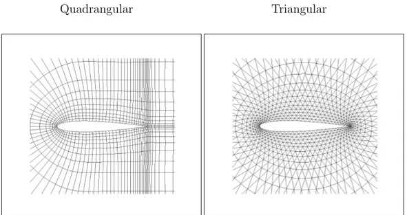
Quadrangular Triangular

Figure 4.1: Computational Grids

In this work, we use a triangular and a quadrangular grid, both displayed in Figure 4.1. The quadrangular mesh is a C-grid with 1792 elements. The triangular mesh is a O-grid with 2048 elements. The far field boundary of both grids is located far away from the aerodynamic surface.

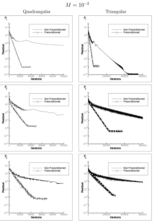
The discussion of the results obtained is split into two different sections, in order to highlight separately two different aspects, the convergence and the accuracy of the solutions.

(46)

• Convergence.

The residual histories versus iteration number were computed to evaluate the effect of the preconditioning technique on the rate of convergence of the solution process. The iteration history is plotted in terms of the L2

norm of the residuals, that represents the change in the solution over an iteration averaged over all the grids points and equations.

The L2 norm is computed as

L2 = s_P N i=1 P_M m=1(δ¯qi,m)2 M ∗ N ,

where N is the total number of grid points and M is the number equa-tions (4 for the 2D Euler Equaequa-tions).

In all figures the residual values are normalized such that the first residual equals 1.

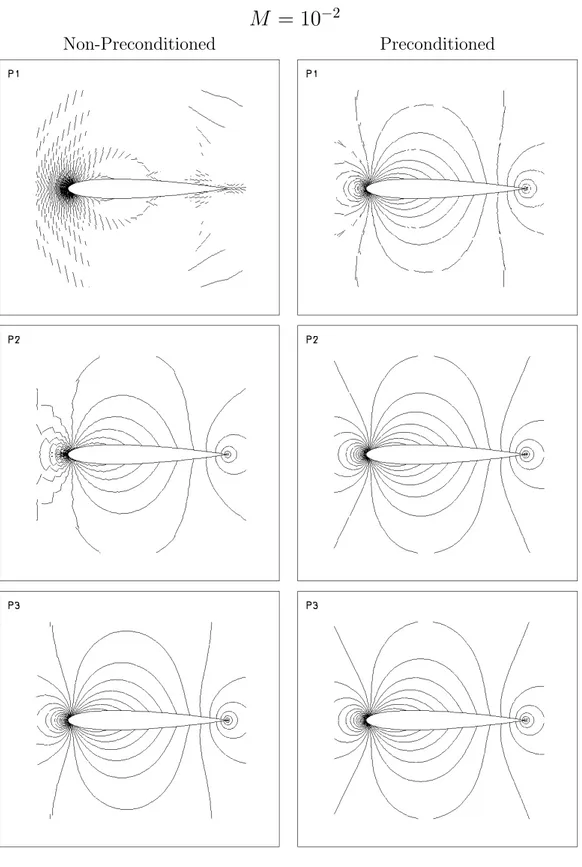
• Accuracy.

The accuracy of the numerical results is examinated from a qualitative and a quantitative point of view.

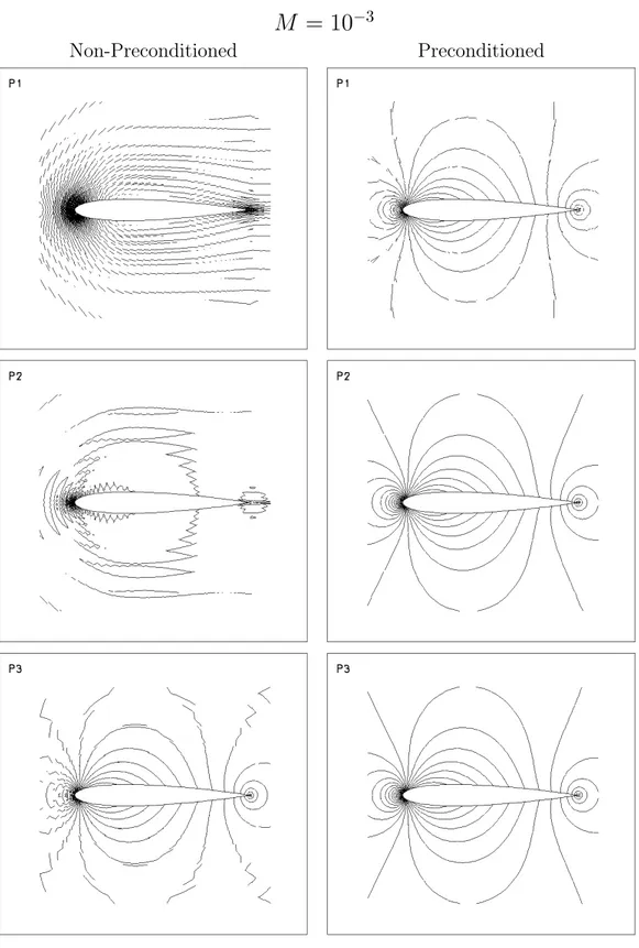
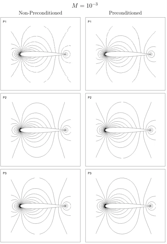
The qualitative analysis is performed showing the normalized pressure

pnorm on the NACA profile. The normalized pressure, pnorm, is defined

as

pnorm = p − pmin

pmax− pmin

.

The quantitative analysis is performed comparing the numerical drag value with the theoretical one (zero the subsonic inviscid flow).

All the computations refer to sufficiently converged solutions and were per-formed in double precision.

4.6.1 Convergence

Figure 4.2 shows the convergence histories for the quadrangular (left) and the triangular (right) grids at a Mach number of M = 10−1_{, using linear (P}

Discontinuous Galerkin Methods for inviscid low Mach number flows

Universit`

a degli studi della Calabria

Dipartimento di Ingegneria Meccanica

Tesi di Dottorato di Ricerca

in Ingegneria Meccanica

Discontinuous Galerkin Methods

for inviscid low Mach number flows

Ing. Alessandra Nigro

Discontinuous Galerkin Methods

for inviscid low Mach number flows

Abstract

Contents

Chapter 1

Introduction

1.1

Motivation

1.2

Background

1.2.1

High-Order Methods

1.2.2

Discontinuous Galerkin Methods

1.2.3

Preconditioning Techniques

1.3

Outline of Thesis

Chapter 2

Physical model

2.1

Conservation Laws

2.1.1

Description

2.1.2

The compressible Euler equations

2.2

The preconditioned compressible Euler

equa-tions

2.3

Non-dimensionalization

Chapter 3

Discontinuous Galerkin

Formulation

3.1

Discretization of the Euler equations

3.2

Numerical Flux function

3.2.1

Roe-average numerical flux

3.2.2

Low Mach behaviour

3.3

Boundary Treatment

3.3.1

Boundary Conditions

3.3.2

Geometry Representation: Curved Boundaries

Chapter 4

Explicit scheme:

Fully Preconditioning technique

for the Euler equations

4.1

Preconditioning matrix

4.2

Time discretization scheme

4.3

Local time stepping

4.4

Preconditioned Roe’s Numerical Flux

4.5

Boundary conditions

4.5.1

Preconditioned far-field

4.5.2

Slip wall

4.6

Results

4.6.1

Convergence