Device-free Counting via OFDM
Signals of Opportunity
Stefania Bartoletti
∗, Andrea Conti
∗, and Moe Z. Win
†∗DE at University of Ferrara, E-mail: [email protected], [email protected] †LIDS at Massachusetts Institute of Technology, E-mail: [email protected]
Abstract—Counting targets (people or things) within a moni-tored area is an important task in emerging wireless applications for smart environments, safety, and security. Counting via passive radars rely on signals of opportunity (i.e., signal already on air for other purposes) to detect and count device-free targets, which is preferable, in terms of privacy and implementation costs, to active radars that rely on dedicated or personal devices. However, conventional radar techniques for multi-target detection require to associate measurements sets to detected targets. Such data association may lead to high dimensionality and complexity even with few targets, despite it is a redundant operation for counting. The need of low dimensionality and complexity calls for the definition of signal features and the development of techniques for their extraction, which enable the association of measured signals directly with the number of targets (namely, crowd-centric algorithms). This paper develops a framework for the design and analysis of crowd-centric algorithms for device-free counting via OFDM signals of opportunity. Preliminary results in simple use cases show the effectiveness of the proposed techniques with respect to individual-centric algorithms.
Index Terms—Counting, signals of opportunity, crowd sensing, OFDM, passive radar.
I. INTRODUCTION
Counting targets, such as people or things, in a mon-itored area enables new important applications for smart environments [1], logistics [2], crowd sensing [3], public safety [4], and environmental monitoring [5]–[7]. Depending on the application and the operating environment, different approaches are considered, including image-based, device-based, and device-free. In all of them, data are collected from multiple sensors and processed to infer the number of targets in a monitored area.
In image-based approaches, the target counting is performed by processing the foreground images collected by one or multiple cameras, after the removal of the background im-ages [8]–[11]. In device-based approaches, the counting is performed by relying on personal or dedicated devices, such as personal smartphone or radio-frequency identification (RFID) tags [12]–[14]. Recently, device-free approaches have been investigated, where the counting is performed by sensing the wireless environment and inferring the number of targets from
This research was supported, in part, by the European Union’s Horizon 2020 research and innovation programme under the Marie Skłodowska-Curie Grant 703893, the Office of Naval Research under Grants N62909-18-1-2017 and N00014-16-1-2141, and the National Science Foundation under Grant CCF-1116501.
reflected signals [5], [14], [15]. Such device-free approaches preserve the privacy of the targets (no data related to the target identity) as well as they reduce the implementation cost with respect to device-based solutions. The capability of detecting and tracking people and things without relying on active devices and through the exploitation of wireless sources already covering the environment would tremendously extend the range of applications and reduce the implementation cost with maximal privacy preservation.
Device-free systems can be classified between active sensor radars (SRs) and passive SRs. Active SRs rely on a network of transmitter-receiver pairs in monostatic or multistatic config-uration [16]–[19]. The signals collected at different receiving nodes are processed to detect multiple targets. Passive SRs rely on illuminators of opportunity and have been employed in the literature for stealth and low-cost tracking. In such a configuration, a network of receiving-only radars receives both the direct signal from an illuminator of opportunity and the signal backscattered by the target.
Previous works on passive radars consider VHF/UHF sta-tions and Wi-Fi base stasta-tions as illuminators of opportunity [20]–[22]. Recently, the orthogonal frequency division mul-tiplexing (OFDM) signals gained interest since they can be efficiently used to detect and locate targets based on Fourier analysis across subsequent blocks, which significantly reduce the computational complexity with respect to processing of other digital signals [23]–[26]. Several signal processing tech-niques have been proposed in the literature to detect the presence and estimate the position of a target based on the received waveforms. For example, time difference-of-arrival (TDOA), frequency difference-of-arrival (FDOA) and angle-of-arrival (AOA) measurements are often adopted in this scenarios where synchronization is not guaranteed between receivers and transmitters [27]–[29].
Current solutions for multi-target detection and tracking systems rely on likelihood calculation and data association for each detected target [17], [18], [30], [31]. Data association is a computationally complex operation (growing exponentially with the number of targets) required for tracking while not necessary for counting systems that aim at estimating only the number of targets disregarding their position. Therefore, there is a growing interest in conceiving methods to count targets from the measured data without estimating the location of each single target (namely, crowd-centric methods) [15], [32], [33].
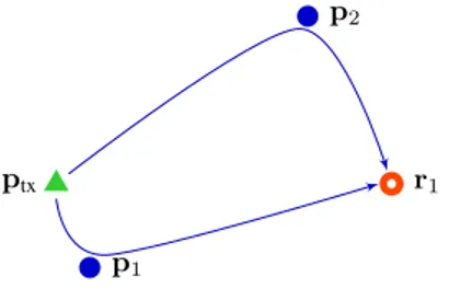
p2
p1
ptx r1
Fig. 1. Example of a portion of operating environment with one transmitter of opportunity (green triangle), one receiver (red circle) and two targets (blue circles).
This paper presents a method to count device-free targets with passive SRs without data association relying only on crowd-centric information. We propose low-complexity count-ing algorithms for OFDM illuminators of opportunity and based on fast Fourier transform (FFT) and OFDM channel estimation.
The remainder of the paper is organized as follows: Sec. II describes the system model; Sec. III introduces the signal processing techniques; and Sec. IV presents a case study and numerical results. Finally, in Sec. V our final remarks are given.
II. SYSTEMMODEL
Consider a network of receiving-only radars with index set R, with the hth radar in position rh (h ∈ R), monitoring an
area illuminated by an OFDM transmitter at ptx. Fig. 1 shows
an example of the operating environment with one transmitter of opportunity, one receiver, two target scatterers and two clutter scatterers. The OFDM transmitter emits a broadcast signal at center frequency fcwith equivalent low-pass version
s(t) =
+∞
X
i=−∞
si(t − i T0) (1)
where, for even number N of subcarriers,
si(t) = N/2−1 X n=−N/2 ai[n]ej2πn∆ft1(−Tcp,T ]{t} (2) in which ai[n] is the ith data symbol on the nth subcarrier,
∆f is the frequency spacing between two adjacent subcarriers,
T0 = T +Tcp, and Tcpis the cyclic prefix time. The transmitted
signal s(t) is decoded and reconstructed as ˆs(t), for example based on the signal collected at a reference receiver (i.e., a reference signal).
Each radar receives the signal after backscattering by all the objects that are present in the operating environment, also referred to as scatterers. The dynamic scatterers (velocity and Doppler shift different than zero) are targets to be counted; the static scatterers (velocity and Doppler shift equal to zero) are present also in the absence of the targets, namely the clutter.
Therefore, the signal collected by the hth radar after multipath propagation is [17]
r(h)(t) = rb(h)(t) + r(h)t (t) + n(h)(t) (3)
where: rb(h)(t) is the signal component related to the back-ground environment due to clutter and direct signal (the same component would be received in the absence of targets, when the area is empty); r(h)t (t) is the signal component related to backscattering from the targets; and n(t) is the noise component.1. An estimate of the background component can
be removed from the received waveform leading to
˘r(h)(t) = r(h)(t) − ˆr(h)b (t) (4) which is the received signal after background removal.
The residual of the background component after background removal depends on the clutter mitigation algorithm, whose analysis is beyond the scope of this paper. Experimental results show that the use of techniques that mitigate the effect of the direct signal and clutter, such as null steering, can attenuate the static background component significantly (even up to 100 dB) and reduce the receiver dynamic range [23], [34]. After ideal clutter removal, the hth received signal becomes
˘r(h)(t) = X k∈K(h) α(h)k ejvkψk(h)˘s(t − τ(h) k ) + n (h)(t) (5)
where: K(h) is the index set of multipath components due to all the targets; α(h)k is the amplitude and τk(h) is the arrival time for the kth path component. In particular, τk(h) = (kptx−
p(k)t k + kp (k)
t − rhk)/c is the arrival time of the component
backscattered by the kth target at p(k)t that propagates over the transmitter-kth target link and the kth target-hth receiver link.2 For the target scatterers, ψ(h)
k = 2πβ
(h)
k fct where
βk(h) = fk(h)/(vfc) = (cos ωt,k+ cos ωr,k) /c where f (h) k is
the Doppler shift, which is considered constant over a block of duration T0, ωt,k is the angle describing the relative direction
between the transmitter and the target, and ωr,k is the angle
describing the relative direction between the target and the kth receiver.3
The aim of a counting system is to estimate the number of target scatterers nt= |K
(h)
t | by processing the received signals
˘
r(h)(t) ∀h ∈ R. The vector
˘r =h˘r(1), ˘r(2), . . . , ˘r(|r|)i (6) 1The noise samples are zero-mean Gaussian random variable (RV) n(h)
j =
n(h)(t
j) ∼ N (0, σ2n) at time tjand the variance σ2n is considered known to
simplify the notation
2The symbol c denotes the speed-of-light and k·k denotes the Euclidean
distance.
3The geometry-based single-bounce model is employed, where the number
of multipath components is equal to the number of scatterers. This is a widely adopted assumption for two reasons: (1) the power related to a double or multiple bounce path is proportional to the product of the radar cross section of two or multiple targets, which is negligible; and (2) this is equivalent to consider a lower spatial resolution, which is a common assumption due to bandwidth limitations that are intrinsic to the hardware that is involved [35].
represents the concatenation of the vectors of received signal samples for each receiver. The length of the vector is nm =
|R| ns, where ns is the number of received signal samples
˘r(h)(nT
s) with n = 0, 1, . . . , ns− 1, which depends on the
sampling time Ts and the observation interval Tobs = nsTs.
The vector pt= h p(1)t , p (2) t , . . . , p (nt) t i (7) is the concatenation of the target position vectors. From (3) and (5), when the background is perfectly removed, i.e. ˆr(h)b (t) = rb(h)(t), it follows that for a given channel instantiation, ˘r(h)is a random vector that depends on a deterministic and unknown parameter vector θ(h)= [p t, α(h), τ(h), v], where v = [v1, v2, . . . , vnt] τ(h) = [τ1(h), τ2(h), . . . , τn(h) t ] α(h) = [α(h)1 , α(h)2 , . . . , α(h)nt ] . (8) and on the noise component n(h)(t). The parameters α(h)
and τ(h), i.e. the arrival time and amplitude of the multipath
components, depend on the channel instantiation. III. SIGNALPROCESSING FORCOUNTING
The proposed method relies on a matched filter receiver, i.e. a bank of correlators tuned to the transmitted waveform given a certain Doppler shift and delay. The number of correlators drives the accuracy and complexity of the counting algorithm. At the hth receiver, each correlator will produce for a delay τ and Doppler shift φ
z(h)(τ, φ) = Z Tobs
0
˘r(h)(t)e−j2πφfcs∗(t − τ )dt (9) where Tobsis the observation time. By considering Tobsas an
integer multiple of T0 and given the OFDM structure of the signal, we have z(h)(τ, φ) = Ti/T0 X i=0 e−jπφfcT N 2 X n=−N 2 h(h)i,nej2πn∆fτ. (10)
If the phase rotation can be approximated as constant within one OFDM block (the product between the Doppler shift and T0 is much smaller than unity), then [23]
h(h)i,n = a∗i[n] Z T 0 e−j2πn∆ft˘r(h)(t + iT0)dt ' X k∈K(h) α(h)k T |ai[n]|2ej2π(ivkψ (h) k fcT0−n∆fτk(h)). (11)
At each receiver, the correlation is calculated for a finite number of tuples (τj, φj) with j ∈ M = 1, 2, . . . , nm, which
represent potential target locations and velocities. In particular, we define Td as the temporal distance between any two pairs
of tentative delays Td = τj− τi∀i, j = 1, 2, . . . , nm and Fd
as the frequentcy distance between any two pairs of tentative Doppler shifts Fd= (φj− φi) ∀i, j = 1, 2, . . . , nm. Therefore,
Td and Fd represent the time and frequency resolution of the
receiver. The signal component backscattered from a target at the tentative position ˜pj such that τj = (kptx− ˜pjk + k ˜pj−
rhk)/c with a Doppler shift φj, will contribute to the received
energy at the jth correlator output z(h)(τj, φj). The output of
all the correlators at the hth receiver is a vector e(h) of nm
energy samples corresponding to the tentative tuples of target locations and velocity. The jth energy sample is given by
e(h)j = z(h)(τj, φj) ' X k∈K(h)t α(h)k T Ti/T0 X i=0 N 2 X n=−N 2 |ai[n]|2 × ej2π(i(vkψ(h)k −φj)fcT0−n∆f(τk(h)−τj)) (12) which represents the energy collected for the jth tuple (τj, φj).
Such an energy has maximum value when φj = vkψ (h) k and
τj = τ (h)
k for any k.
The estimated number of targets ˆn(h)t is obtained at the hth
receiver from e(h). The final estimate for the number of targets is the mean value of the number estimated by the different sensors ˆ nt= 1 ns X h∈R ˆ n(h)t . (13)
To calculate ˆn(h)t , we propose two possible algorithms, a maximum bin search (MBS) and threshold crossing search (TCS). For both the algorithms, a threshold for each energy sample is defined by the vector ξ = [ξ1, ξ2, . . . , ξNm]. The estimated number of targets is initialized for each sensor as ˆn(h)t,0 = 0, and the energy vector is initialized as ˜e0 =
[e(h)1,0, e(h)2,0, . . . , e(h)n
m,0]. At the kth step, the number of targets is estimated from ˜ek and ˜ek is updated through the path loss
law, which is known or learned through measurements. In particular, given the path loss law, a value αj can be
associated to the tentative arrival time τj as
αj= Q (h) j exp(τj/γ) (14) where Q(i)k = 10 Pj(h)/10 Pnt k=1τj/γ , (15)
γ is the power decay constant, and Pj(h) is the received signal strength (RSS) for a target at ˜pj with respect to the hth
receiver, i.e., considering the path-loss and the radar cross section (RCS) of the corresponding scatterer [17].4
The value αj can be used to calculate the expected value
of e(h)j when a target is at ˜pj. If one or multiple targets are
detected at ˜pj, its energy contribution is removed from the
4The RCS measures the power density that the object reflects with respect
to the incident power, in relation to scatterer orientation, material, and size [18], [36], [37].
Algorithm 1 Maximum Bin Search 1: k ← 0 2: nˆ(h)t,0 ← 0 3: ˜e0,i← e (h) i ∀i ∈ M 4: ˆı ← argmaxi{˜e0,i> ˜e0,j∀j 6= i} 5: while ˆn(h)t,k and eˆ(h)ı > ξˆı do 6: k ← k + 1 7: nˆ(h)t,k ← ˆn(h)t,k−1+ 1 8: Update ˜ek from (16) 9: ˆı ← argmaxi{˜ek,i> ˜ek,j∀j 6= i}
Algorithm 2 Threshold Crossing Search
1: k ← 0 2: nˆ(h)t,0 ← 0 3: ˜e0,i← e (h) i ∀i ∈ M 4: ˆı ← min{i ∈ M : ˜e0,i> ξi} 5: while ˆn(h)t,k and ˆı 6= ∅ do 6: k ← k + 1 7: nˆ(h)t,k ← ˆn(h)t,k−1+ 1 8: Update ˜ek from (16) 9: ˆı ← min{i ∈ M : ˜ek,i> ξi}
energy vector starting from αj as
˜ ek= ˜ek−1− ˜αˆıT Ti/T0 X i=0 N 2 X n=−N 2 |ai[n]|2 × ej2π(i(φˆı−φj)fcT0−n∆f(τˆı−τj)). (16) The MBS is presented in Alg. 1. At each iteration, the MBS algorithm first searches for the maximum value among all the bins with index j ∈ M. If such maximum value is above the corresponding threshold, the number of targets is updated, the energy vector is updated by considering the , and the search is made again. The algorithms is terminated when the energy bins are all below the threshold or a maximum number of detected targets nmax is reached.
The TCS is presented in Alg. 2. At each iteration, the TCS algorithm searches for the first value among all the bins with index j ∈ M that overcomes the corresponding threshold. If such maximum value is above the corresponding threshold, the number of targets is updated, the energy vector is updated, and the search is made again. The algorithms is terminated when the energy bins are all below the threshold or a maximum number of detected targets nmax is reached.
IV. CASESTUDY
Consider a squared monitored environment of 10 m × 10 m with one transmitter in the center ptx = [5, 5] m and four
receivers at the corners, r1 = [0, 0], r2 = [0, 10], r3 =
[10, 10], and r4 = [10, 0], with ns = 4. The maximum
number of targets is nmax = 10 and results are obtained
via Monte Carlo simulation by varying the number of targets nt= {0, 1, 2, . . . , nmax} and considering the targets uniformly
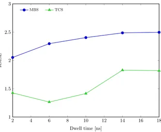
Fig. 2. RMSE for different values of Td.
Fig. 3. Counting error outage for the MBS and TCS algorithms.
distributed in the monitored environment. The transmitted signal is a Wi-Fi signal, with bandwidth B = 20 MHz, number of carriers N = 52, carrier spacing ∆f= 312.5 KHz
according to the IEEE 802.11 standard. The symbols are perfectly reconstructed and ideal clutter removal is considered. Counting is performed with the MBS and TCS algorithms. The performance is evaluated in terms of counting error outage Pceo(n), i.e. the percentage of times that the counting error
|ˆnt − nt| is above n and root-mean-square of the counting
error (RMSE). The resolution of the energy vector varies, with Td = 2, 4, . . . , 18 ns, whereas the target velocity is assumed
as known. The threshold vector is chosen as the one the minimizes the RMSE.
Fig. 2 shows the RMSE for different values of Td. It can
be observed that the TCS outperforms the MBS for all the values of Td considered. For example, for the same value of
Td = 6 ns, the root-mean-square error (RMSE) is 2.05 with
MBS and 1.42 with TCS. Furthermore, the RMSE increases with Tdfor the MBS case, and goes from 2.05 with Td = 2 ns
with Td= 6 ns for the TCS case. Therefore, the time resolution
has a important impact on the counting performance and its optimal value depends on the algorithm employed.
Fig. 3 shows the counting error outage Pceo(n) as a function
of n for the TCS and MBS algorithms. Results are obtained with Td = 2 ns in the MBS case and with Td = 6 ns for
the MBS case, which represent the best cases in terms of RMSE according to Fig. 2. It can be observed that the MBS is outperformed by the TCS. In particular, the probability that the counting error is above 2 is 0.19 for the MBS and 0.04 for the TCS.
V. FINALREMARK
A device-free counting system that relies on OFDM signals of opportunity is presented. The proposed counting system does not require data association and is based on crowd counting algorithms. The counting system performance is evaluated in a simple case study with Wi-Fi signals varying the number of targets and considering two different algorithms based on maximum search and threshold crossing. Results show the importance of the choice of time resolution for the counting performance.
REFERENCES
[1] G. Cardone, P. Bellavista, A. Corradi, C. Borcea, M. Talasila, and R. Curtmola, “Fostering participaction in smart cities: A geo-social crowdsensing platform,” IEEE Commun. Mag., vol. 51, no. 6, pp. 112– 119, Jun. 2013.
[2] X. Wang, S. Yuan, R. Laur, and W. Lang, “Dynamic localization based on spatial reasoning with RSSI in wireless sensor networks for transport logistics,” Sensors and Actuators A: Physical, vol. 171, no. 2, pp. 421– 428, Nov. 2011.
[3] F. Zabini and A. Conti, “Inhomogeneous Poisson sampling of finite-energy signals with uncertainties in Rd,” IEEE Trans. Signal Process.,
vol. 64, no. 18, pp. 4679–4694, Sep. 2016.
[4] S. M. George, W. Zhou, H. Chenji, M. Won, Y. O. Lee, A. Pazarloglou, R. Stoleru, and P. Barooah, “Distressnet: A wireless Ad Hoc and sensor network architecture for situation management in disaster response,” IEEE Commun. Mag., vol. 48, no. 3, pp. 128–136, Mar. 2010. [5] E. Cianca, M. D. Sanctis, and S. D. Domenico, “Radios as sensors,”
IEEE Internet of Things Journal, 2016, to appear.
[6] A. Basalamah, “Sensing the crowds using bluetooth low energy tags,” IEEE Access, vol. 4, pp. 4225–4233, Aug. 2016.
[7] S. Savazzi, S. Sigg, M. Nicoli, V. Rampa, S. Kianoush, and U. Spagno-lini, “Device-free radio vision for assisted living: Leveraging wireless channel quality information for human sensing,” vol. 33, no. 2, pp. 45– 58, Mar. 2016.
[8] Y. L. Hou and G. K. H. Pang, “People counting and human detection in a challenging situation,” IEEE Transactions on Systems, Man, and Cybernetics - Part A: Systems and Humans, vol. 41, no. 1, pp. 24–33, Jan 2011.
[9] N. C. Tang, Y. Y. Lin, M. F. Weng, and H. Y. M. Liao, “Cross-camera knowledge transfer for multiview people counting,” IEEE Transactions on Image Processing, vol. 24, no. 1, pp. 80–93, Jan 2015.
[10] B. K. Dan, Y. S. Kim, Suryanto, J. Y. Jung, and S. J. Ko, “Robust people counting system based on sensor fusion,” IEEE Transactions on Consumer Electronics, vol. 58, no. 3, pp. 1013–1021, August 2012. [11] A. B. Chan and N. Vasconcelos, “Counting people with low-level
fea-tures and Bayesian regression,” IEEE Transactions on Image Processing, vol. 21, no. 4, pp. 2160–2177, April 2012.
[12] F. Guidi, N. Decarli, S. Bartoletti, A. Conti, and D. Dardari, “Detection of multiple tags based on impulsive backscattered signals,” vol. 62, no. 11, pp. 3918–3930, Nov. 2014.
[13] E. Vattapparamban, B. S. Ciftler, I. Guvenc, K. Akkaya, and A. Kadri, “Indoor occupancy tracking in smart buildings using passive sniffing of probe requests,” in 2016 IEEE International Conference on Communi-cations Workshops (ICC), May 2016, pp. 38–44.
[14] S. Depatla, A. Muralidharan, and Y. Mostofi, “Occupancy estimation using only WiFi power measurements,” IEEE Journal on Selected Areas in Communications, vol. 33, no. 7, pp. 1381–1393, July 2015. [15] X. Quan, J. W. Choi, and S. H. Cho, “In-bound/out-bound detection of
people’s movements using an IR-UWB radar system,” in Int. Conf. on Electronics, Information and Communications (ICEIC), Kota Kinabalu, Malaysia, Jan. 2014, pp. 1–2.
[16] M. I. Skolnik, “An analysis of bistatic radar,” vol. ANE-8, no. 1, pp. 19–27, Mar. 1961.
[17] ——, Radar Handbook, 2nd ed. McGraw-Hill Professional, Jan. 1990. [18] V. S. Chernyak, Fundamentals of Multisite Radar Systems: Multistatic Radars and Multiradar Systems, 1st ed. New York: CRC Press, Sep. 1998.
[19] E. Paolini, A. Giorgetti, M. Chiani, R. Minutolo, and M. Montanari, “Localization capability of cooperative anti-intruder radar systems,” EURASIP Journal on Advances in Signal Processing, vol. 2008, pp. 1–14, 2008, article ID 726854, doi:10.1155/2008/726854.
[20] M. Glende, J. Heckenbach, H. Kuschel, S. Mueller, J. Schell, and C. Schumacher, “Experimental passive radar systems using digital illu-minators (DAB/DVB-T),” in Proc. Int. Radar Symp, Cologne, Germany, Sep. 2007, pp. 411–417.
[21] H. Kuschel, J. Heckenbach, S. Mueller, and R. Appel, “On the potentials of passive, multistatic, low frequency radars to counter stealth and detect low flying targets,” in Proc. IEEE Radar Conf., Rome, Italy, May 2008, pp. 1443–1448.
[22] C. Coleman, H. Yardley, and R. Watson, “A practical bistatic passive radar system for use with DAB and DRM illuminators,” in Proc. IEEE Radar Conf., Rome, Italy, May 2008, pp. 1514–1519.
[23] C. R. Berger, B. Demissie, J. Heckenbach, P. Willett, and Z. Shengli, “Signal processing for passive radar using OFDM waveforms,” vol. 4, no. 1, pp. 226–238, Feb. 2010.
[24] C. R. Berger, S. Zhou, and P. Willett, “Signal extraction using com-pressed sensing for passive radar with OFDM signals,” in Proc. Int. Conf. Inf. Fusion (FUSION), Cologne, Germany, Jun. 2008, pp. 1514– 1519.
[25] S. Bartoletti, A. Conti, and M. Z. Win, “Towards counting via passive radar using OFDM waveforms,” in Proc. IEEE Int. Conf. Commun., Paris, France, May 2017, pp. 803–808.
[26] ——, “Device-free counting via wideband signals,” IEEE J. Sel. Areas Commun., vol. 35, no. 5, pp. 1163–1174, May 2017.
[27] K. C. Ho, L. Xiaoning, and L. Kovavisaruch, “Source localization using TDOA and FDOA measurements in the presence of receiver location errors: Analysis and solution,” vol. 55, no. 2, pp. 684–696, Feb. 2007. [28] M. Z. Win, A. Conti, S. Mazuelas, Y. Shen, W. M. Gifford, D. Dardari,
and M. Chiani, “Network localization and navigation via cooperation,” IEEE Commun. Mag., vol. 49, no. 5, pp. 56–62, May 2011.
[29] A. Conti, M. Guerra, D. Dardari, N. Decarli, and M. Z. Win, “Net-work experimentation for cooperative localization,” IEEE J. Sel. Areas Commun., vol. 30, no. 2, pp. 467–475, Feb. 2012.
[30] F. Meyer, P. Braca, P. Willett, and F. Hlawatsch, “Tracking an unknown number of targets using multiple sensors: A belief propagation method,” in Proc. FUSION-16, Heidelberg, Germany, Jul. 2016, pp. 719–726. [31] J. Williams and R. Lau, “Approximate evaluation of marginal association
probabilities with belief propagation,” IEEE Trans. Aerosp. Electron. Syst., vol. 50, no. 4, pp. 2942–2959, Oct. 2014.
[32] J. W. Choi, J. H. Kim, and S. H. Cho, “A counting algorithm for multiple objects using an IR-UWB radar system,” in IEEE Int. Conf. on Net. Infrastr. and Digital Content, Beijing, China, Sep. 2012, pp. 591–595. [33] J. He and A. Arora, “A regression-based radar-mote system for people
counting,” in Pervasive Computing and Communications (PerCom), 2014 IEEE International Conference on, Louis Missouri, USA, Mar. 2014, p. 95102.
[34] H. D. Griffiths and C. J. Baker, “Passive coherent location radar systems. part 1: performance prediction,” IEE Proc. Radar, Sonar Navigation, vol. 152, no. 3, pp. 153–159, Jun. 2005.
[35] A. Meijerink and A. F. Molisch, “On the physical interpretation of the saleh-valenzuela model and the definition of its power delay profiles,” vol. 62, no. 9, pp. 4780–4793, Sep. 2014.
[36] S. Bartoletti, A. Conti, and A. Giorgetti, “Analysis of UWB radar sensor networks,” Cape Town, South Africa, May 2010, pp. 1–6.
[37] S. Bartoletti, A. Giorgetti, M. Z. Win, and A. Conti, “Blind selection of representative observations for sensor radar networks,” IEEE Trans. Veh. Technol., vol. 64, no. 4, pp. 1388–1400, Apr. 2015.