DEPT. OFCOGNITIVESCIENCE, PSYCHOLOGY, EDUCATION AND CULTURALSTUDIES
G
RADUATES
TUDIES INC
OGNITIVES
CIENCE- XXXIII C
OURSENeural Models of Contextual
Semantic Disambiguation
Arianna Maria Pavone
A DISSERTATION
SUBMITTED TO DEPARTMENT OF COGNITIVE SCIENCE,
PSYCHOLOGY,EDUCATION AND CULTURAL STUDIES AND THE COMMITTEE ON GRADUATE STUDIES
OFUNIVERSITY OFMESSINA IN FULFILLMENT OF THE REQUIREMENTS
FOR THE DEGREE OF
DOCTOR OF PHILOSOPHY IN COGNITIVE SCIENCE
DIRECTOR OFGRADUATESTUDIES ADVISOR
a dissertation for the degree of Doctor of Philosophy.
Prof. Alessandra Falzone (Director of Graduate Studies)
I certify that I have read this dissertation and that, in my opinion, it is fully adeguate in scope and quality as a dissertation for the degree of Doctor of Philosophy.
Prof. Alessio Plebe (Advisor)
Approved for the University Committe on Graduate Studies.
In human language several ambiguities cannot be resolved without simultaneously rea-soning about an associated context. Often, the context can be best catpured from the visual scene referred by the sentence. If we consider the sentence “I take a photograph of a chimpanzee in my pajamas”, looking at language alone, it is unclear if it is the person or the chimpanzee wearing the pajamas.
In this dissertation we focus on the contextual effects on semantics: on the one hand we investigate such contextual effects on a disambiguation task using neural computa-tional simulation; on the other hand we propose a novel context sensitive cognitive ac-count of similarity.
Going a little more in detail in our disambiguation task, provided with a sentence, admitting two or more candidate interpretations, and an image that depicts the content of the sentence, it is required to choose the correct interpretation of the sentence depending on the image’s content. Thus we address the problem of selecting the interpretation of an ambiguous sentence matching the content of a given image.
This type of inference is frequently called for in human communication that occurs in a visual environment, and is crucial for language acquisition, when much of the linguistic content refers to the visual surroundings of the child [8, 11].
This kind of task is also fundamental to the problem of grounding vision in language, by focusing on phenomena of linguistic ambiguity, which are prevalent in language, but typically overlooked when using language as a medium for expressing understanding of visual content. Due to such ambiguities, a superficially appropriate description of a
vi-sual scene may in fact not be sufficient for demonstrating a correct understanding of the relevant visual content.
Regarding our new contextual account of similarity, we will suggest that most of the traditional similarity models which have been proposed over the years can converge on a generalized model of similarity in which the context plays a fundamental role in order to overcome all the criticisms raised over the years to each of the traditional similarity models.
From the neurocomputational point of view, our models are based on the Eliasmith’s Neural Engineering Network (NEF) [27] and Nengo1, the python library which serves as an implementation of the NEF. The basic semantic component within NEF is the so-called Semantic Pointer Architecture (SPA) [129], which determines how the concepts are represented as dymanic neural assemblies.
Preface i
Table of Contents iii
Introduction 2
1 A Framework for Neural Semantics 6
1.1 NEF - A Framework for simulating the brain . . . 10
1.1.1 The Representation’s Principle . . . 11
1.1.2 The Transformations’s Principle . . . 12
1.1.3 The Dynamic’s principle . . . 13
1.2 Nengo . . . 13
1.2.1 The main Nengo’s objects . . . 14
1.3 The Representation’s Principle with Nengo . . . 16
1.3.1 Representation with a single neuron . . . 16
1.3.2 Representation with a pair of neurons . . . 19
1.3.3 Representation with a Neural Population . . . 22
1.3.4 Representation of a pair of signals . . . 24
1.3.5 Representation of the sum of two signals . . . 25
1.4 The Transformation Principle with Nengo . . . 28
1.4.1 An amplification channel . . . 28
1.4.2 Arithmetic operations . . . 30
1.5 Dynamic Transformations with Nengo . . . 33
1.5.1 Simulation of a integrator . . . 33
2 The Semantic Pointer Architecture 35 2.1 The semantic pointer . . . 35
2.1.1 Physical characterization of a semantic pointer . . . 36
2.1.2 Mathematical characterization of a semantic pointer . . . 36
2.1.3 Functional characterization of a semantic pointer . . . 38
2.1.4 The semantic pointer at a glance . . . 40
2.2 Deep semantics and superficial semantics . . . 40
2.2.1 Characterization of partial semantics . . . 41
2.2.2 Hierarchical structure of semantic cognitive processes . . . 42
3 A Computational Model of the Neural Circuits for Contextual Behaviour 49
3.1 The Brain as a Context Machine . . . 50
3.2 Neural Circuits for Contextual Behaviour . . . 51
3.3 Role and Anatomy of the CA3 Region . . . 54
3.4 A SPA Model of the CA3 Region . . . 56
3.4.1 Paired Item-Item and Item-Context Association Path . . . 56
3.4.2 Recurrent Collaterals Path . . . 59
3.5 Preliminary Evaluation . . . 60
4 Visual Resolution of Linguistic Ambiguities 64 4.1 Definition of the Task . . . 66
4.2 The ambiguity testbed . . . 68
4.3 Background . . . 70
4.4 Our Model . . . 72
4.5 Experimental results . . . 75
5 A Context Sensitive Account of Similarity Based on the SPA 80 5.1 Why Similarity? . . . 80
5.1.1 Background . . . 81
5.1.2 Our Proposal . . . 82
5.2 Models of Similarity . . . 84
5.2.1 Geometric Models . . . 84
5.2.2 Feature Based Models . . . 86
5.2.3 Alignment Based Models . . . 87
5.2.4 Transformational Models . . . 87
5.3 An Account of Similarity based on the SPA . . . 88
5.3.1 An Account of Similarity based on the SPA Framework . . . 88
5.4 Criticisms to Standard Models and their Settlement . . . 93
5.4.1 The reflexive relation . . . 93
5.4.2 The symmetric relation . . . 95
5.4.3 Triangle inequality . . . 97
5.4.4 Limit on the number of closest neighbors . . . 99
5.4.5 Unstructured representations in features based models. . . 100
6 Conclusions and Future Works 102 6.1 General Consideration . . . 103
6.2 The Winograd Challenge . . . 104
6.3 Gardenfors’ Conceptual Spaces . . . 105
In recent years, a number of different disciplines have begun to investigate the funda-mental role that context plays in different cognitive phenomena. The problem of context spans from the abstract level of semantics down to the level of neural representations. It has increasingly been studied also for its role in influencing mental concepts and, more specifically, linguistic communication has been the area of study that has traditionally explored these issues.
The term context is not easy to define: it is something that cannot be specified in-dependently of a specific frame and it may play quite different roles within alternative research paradigms. In wider terms, as stated by [38], we can define the context as a ”frame that surrounds the event and provides resources for its appropriate interpretation”. However, in order to obtain a more complete understanding of what context stands for, it is necessary to investigate how it interacts with cognitive phenomena at three different levels: the linguistic, the cognitive and the neural level [99].
There is a long tradition in linguistics and pragmatics which invokes context to help account for aspects of meaning in language that go beyond the scope of semantics. The main elements of context has roots that dates back to the past, and regards the degree to which truth-functional semantics depends on context. Gottlob Frege raised the point in his uncompleted 1897 volume Logik, and though he was not explicitly using the term context, he underlined how for many expressions, fixing their truth value requires supplemental information, coming from the circumstances, the ”frames”, in which such expressions are pronounced.
The first clear elucidation of the dependence of language on context was proposed by [120]. He takes up Frege’s idea that a word has meaning only if related to the meaning of the whole sentence and if its meaning is perceived by both interlocutors, speaker and listener.
de-pendent on context. [7] has been one of the first to underline how difficult it is to conceive them as stable subjective entities, while it appears more appropriate to think of categories as dynamically constructed and tailored to specific contexts, or as ad hoc categories. A re-cent review of studies of the cognitive perspective on the linguistic issue of context can be found in [2]. Just as in the strictly linguistic domain, they find in the wider cognitive view a variety of positions, some that minimize the destabilizing effect context has on con-cepts, such as that of [71], or others that assume a more intermediate position such as that of [82], that while acknowledging the fundamental role context might play in concepts, sustain that a characterizing stable nucleus of mental concepts is also a part.
From the neuroscientific point of view, the context has started to have a certain rel-evance and the issue regards whether the activation of neurons, in response to the same stimuli, can significantly change due to contextual factors, with increasing studies on the functioning of the hippocampal region, an area traditionally considered as being a site of contextual effects processing. In particular, signs of environmental context are repre-sented in the place cell, and can influence discrimination decisions between visual stimuli and emotional fear responses. Neurons in area CA1 (primary area of the Cornu Ammonis) instead codify contextual overlap of a temporal nature, so that memories of events taking place in brief temporal sequences subsequently have facilitated reciprocal re-activation. Cognitive neuroscience is now starting to consider in a systematic way how context in-teracts with neural responses [126]. The way context drives language comprehension depends on the effects of context on the conceptual scaffolding of the listener, which in turn, is the result of his neural responses in combination to context.
The kind of ambiguity addressed in this work is the canonical case of structural ambi-guity, technically known as Prepositional Phrase Attachment, where a sentence includes a prepositional phrase that can be attached to more than one higher level phrases [50]. The attachment resolution is context dependent, we deal specifically with the case when depends on the visual context.
In addressing the analysis of contextual effects with a neuro-computational approach, a preliminary question concerns the optimal way to encode concepts in clusters of ac-tivation vectors. A theoretical criterion to ascertain that the chosen coding is effective,
and cognitively plausible, is to verify how the coding behaves in front of one of the main relationships that exists between concepts: semantic similarity.
The fact that human assessments of similarity are fundamental to cognition is a widely shared opinion. Similarity, is fundamental for learning, knowledge and thought, since only our sense of similarity allows us to order things into kinds so that these can function as stimulus meanings. Reasonable expectation depends on the similarity of circumstances and on our tendency to expect that similar causes will have similar effects.
On the other hand the context plays a fundamental role in the perception of the similar-ity between two different concepts: depending on the context in which they are compared, two entities can appear more or less similar to each other.
For the reasons reported above, although not central to the main problem of this work, a specific study on this aspect was therefore included in this thesis, proposing a context sensitive similarity model based on SPA.
This dissertation is organized as follows. In Chapter 1 we introduce the Neural En-gineering Framework (NEF), a general methodology that allows you to build large-scale, biologically plausible, neural models of cognition. It acts as a neural compiler: you specify the properties of the neurons, the values to be represented, and the functions to be computed, and it solves for the connection weights between components that will perform the desired functions. Importantly, this works not only for feed-forward computations, but recurrent connections as well. It incorporates realistic local error-driven learning rules, al-lowing for online adaptation and optimization of responses. In Chapter 1 we also present Nengo, a Python library that allows the construction and simulation of large-scale brain models using the NEF method.
In Chapter 3 we schematically discuss the information flow and interactions among the main brain regions involved in contextual behavior, as emerged by recent advancement in neurosciences and present a circuit for simplified model of the CA3 hippocampal region involved in the retrieval of semantic relations between two items (item-item association) and between an item and a context (item-context association).
In Chapter 4 we focus on the contextual effects of visual scenes on semantics, inves-tigated using neural computational simulation. Specifically we address the problem of
selecting the interpretation of sentences with an ambiguous prepositional phrase, match-ing the context provided by visual perception. More formally, provided with a sentence, admitting two or more candidate resolutions for a prepositional phrase attachment, and an image that depicts the content of the sentence, it is required to choose the correct resolu-tion depending on the image’s content. We evaluated the ability of our model in resolving linguistic ambiguities on the LAVA (Language and Vision Ambiguities) dataset, a corpus of sentences with a wide range of ambiguities, associated with visual scenes.
Finally in Chapter 5 we propose a context sensitive plausible model of semantic sim-ilarity, according with the main guidelines of the other traditional models known in lit-erature, based on the Semantic Pointer Architecture which is at the basis of the NEF. We show how our new proposed model is able to give a solution to traditional criticisms against traditional models of similarity.
1
A Framework for Neural Semantics
A first critical choice is the identification of a suitable neural framework to be adopted all along this work. The two main requirements we seek is the biological plausibility and the possibility of modeling at a level enough abstract to deal with full images and with words in sentences. The two requirements are clearly in stark contrast to each other. On the extreme of biological plausibility we find neural simulators describing the current flow in neural compartments, like NEURON [43] and GENESIS [13], used for realistic simula-tions of small volumes of the brain, as done in the European Brain Project [78]. There is no hope of investigating cognitive phenomena with such models. On the other extreme of high level of abstraction and aptitude towards the investigation of cognitive phenom-ena there is the tradition of so-called connectionism [117]. These artificial neural models become widespread around the 1990s in cognitive science, especially in the psychology of language development [29, 72], but their application was limited to highly simplified small experiments, using toy visual and linguistic stimuli.
Today the legacy of connectionism has been taken up by the family of algorithms collected under the name deep learning. Unlike the former artificial neural networks, deep learning models succeeds in highly complex cognitive tasks, reaching even human-like performances in some visual tasks [137]. However, the level of biological plausibility
of deep learning algorithms is in general even lower than in connectionism, these models were developed with engineering goals in mind, and exploring cognition is not in the agenda of this research community [100]. In our model we will also include a very simple deep learning component, but only for the low-level analysis of the images. This choice makes the model simpler, by exploiting the ease of deep learning model in processing visual stimuli. It would have been easy to solve also the crucial part of our problem, the semantic disambiguation, through deep learning, but this would have been of little value as a cognitive model.
An interesting compromise between biological plausibility and level of abstraction is Topographica [10], designed with the main purpose of simulating cortical maps. Al-though it has been successfully used in exploration of neural semantics at the level of early language acquisition [98], Topographica finds its best use in modeling responses in visual areas. Currently, the neural framework that can simulate the widest range of cog-nitive tasks, by adopting a unified methodology with a reasonable degree of biological plausibility, is Nengo (Neural ENGineering Objects) [27]. The idea behind Nengo dates back to 2003, thanks to the former NEF (Neural Engineering Framework) [28], which defines a general methodology for the construction of large cognitive models, informed by a number of key neuroscientific concepts. In brief, the three main such concepts are the following:
• the Representation’s principle: neural representations are defined by the combina-tion of nonlinear encoding of spikes over a populacombina-tion of neurons, and weighted decoding over the same populations of neurons and over time;
• the Transformation’s principle: transformations of neural representations are func-tions of the variables represented by neural populafunc-tions. Transformafunc-tions are deter-mined using an alternately weighted decoding;
• the Dynamic’s principle: neural dynamics are characterized by considering neural representations as state variables of dynamic systems. Thus, the dynamics of neuro-biological systems can be analyzed using control (or dynamics systems) theory. According to the listed principles, the basic computational object in Nengo is a
popu-lation of neurons that collectively can represent a multidimensional entity. The meaning-ful entity is retrieved from the neural activation by the following equation (pp.395–397 of [27]): ~x = N,M
∑
i, j e− t−ti,m τ d~i (1.1)where N is the number of neurons in the population, and M is the number of spikes that happen in the time windows of the computation; ti,m is the time when the i-th neuron in
the population has fired for the m-th time; ~diis the i-th raw of the N × D decoding matrix ~Dwith D the dimension of the entity to be represented; τ is the time constant of decay of the postsynaptic activation. The activity of the neurons in a population depends from the encodingof their input that can be multidimensional with a dimension different from D.
A fundamental extension of the general neural population, ruled by equation (1.1), is the the Semantic Pointer Architecture (SPA), used when representing entities at higher cognitive level, i.e. conceptual and linguistic. In addition to the encoding and the decod-ing features, SPA structures allow a number of high level operations, that may correspond to conceptual manipulation, with some degree of biological plausibility. The foundation of these conceptual operations is in the mathematics of holographic representations, as theorized by Tony [97]. One of the basic operations is the binding of two SPA, computed by circular convolution (p.406 of [27]):
~x ~~y = F−1(F (~x) · F (~y)) (1.2) whereF is the discrete Fourier transform and F−1is its inverse, and · is the element-wise multiplication. Informally, SPA together with its associated operations, can be thought as a neural process that compresses information in other neural processes to which it points and into which it can be expanded when needed, providing shallow meanings through symbol-like relations to the world and other representations, and expanding to provide deeper meanings with relations to perceptual, motor, and emotional information, support complex syntactic operations. They also help to control the flow of information through a cognitive system to accomplish its goals. Thus semantic pointers have semantic, syntactic, and pragmatic functions, just like the symbols in a rule-based system, but with a highly distributed, probabilistic operation.
There are several reasons that have lead to this choice, one of the main reasons is that Nengo is developed from the NEF (Neural Engineering Framework), The NEF defines a general methodology for the construction of large cognitive models, and in particular of biologically plausible neural models. It acts as a neural compiler, that is it allows to specify the properties of the neurons, the values to be represented, the functions to be cal-culated and allows to find solutions for the connection weights between the components of the network that will perform the required functions. This system also allows to sim-ulate complex dynamic models such as integrators, oscillators, and incorporates realistic error-based learning rules, allowing the adaptation and optimization of responses. The motivations that drive our research interest towards the creation of biologically plausible cognitive models and towards realistic models of neurons are increasingly shared by the scientific community.
In the first place, having biologically realistic (and plausible) models allows us to bet-ter verify the theories on which these models are based. If you want to understand exactly how a brain works, it is not enough to reproduce its correct behavior; it is necessary that this be done in exactly the same way that the brain would do it. That is, you should be able to have models of activation and neural connectivity that are comparable to natural ones. This drives our interest toward NEF models rather than algorithmic models of reasoning simulation.
In this first chapter I will limit my introduction to the basic elements of Nengo, and the important role that they have within my work. I will not include here one compo-nent, the Semantic Pointer Architecture, because it is charged by non trivial philosophical implications, and it deserves a deeper discussion in a next chapter. This first chapter is dedicated to the general explanation of how the main components of Nengo work, I will also show some examples of computational calculation through the use of some math-ematical functions implemented in Python that will show us some essential arithmetic operations.
1.1
NEF - A Framework for simulating the brain
The NEF is the acronym that indicates the Neural Engineering Framework. The idea be-hind the NEF dates back to 2003, thanks to a book written by Eliasmith and Charles H. Anderson, entitled Neural Engineering [27] were many mathematical models and theories on how the biological natural systems were able to implement numerous dynamic func-tions were presented. From these theories the NEF takes origin. Eliasmith and Anderson focused on ”low-level” systems, including parts of the brainstem involved in controlling stable eye position. They used these methods to better understand more general issues about neural functions, such as how the variability of neural spike trains and the timing of individual spikes relate to information that can be extracted from spike patterns.
The NEF lends itself to a wide variety of applications. The reason for this is because it does not make assumptions about what specific functions the brain performs. Rather, it is a set of three principles that can help determine how the brain performs some given function. As John Miller once suggested, the NEF is a kind of neural compiler [25].
If you have an idea about the high-level function of the brain area in which you are interested, and you know some information about how neurons respond in that area, the NEF provides a way of connecting populations or layers of neurons together to realize that function. This, of course, is exactly what a compiler does for computer programming languages.
However, things are not so simple when it comes to the brain and its functions, build-ing models with the NEF can be an iterative process: first, you gather from the neural system and generate a hypothesis about what it does; then you build a model using the NEF and see if it behaves like the real system; then, if it does not behave consistently with the data, you alter your hypothesis or perform experiments to figure out why the two are different. What the NEF offers is a systematic method for performing these steps in the context of neurally realistic models.
As I mentioned previously, the core of NEF are three principle, that will be shown in the following section:
• The Representation’s principle: neural representations are defined by the combina-tion of nonlinear encoding (exemplified by neuron tuning curves and neural spiking)
and weighted linear decoding (over populations of neurons and over time);
• The Transformation’s principle: transformations of neural representations are func-tions of the variables represented by neural populafunc-tions. Transformafunc-tions are deter-mined using an alternately weighted linear decoding;
• The Dynamic’s principle: neural dynamics are characterized by considering neural representations as state variables of dynamic systems. Thus, the dynamics of neu-robiological systems can be analyzed using control (or dynamics systems) theory. These three principles will be described one by one and practical examples will be pro-vided on how they work.
1.1.1
The Representation’s Principle
A central principle in NEF is that of adaptability. We can adapt the theoretical informa-tion we have about codes, to understanding the representainforma-tion of neural systems. Codes are defined in terms of complimentary encoding and decoding procedures between two alphabets, as for the morse alphabet for example. To encode it, it is necessary to find a link between the set of lines and the dots that compose it and the alphabet in roman let-ters. The encoding procedure is the mapping from the roman alphabet to the morse code alphabet, and the decoding procedure is its inverse [73].
To characterize representation in a neural system, we must identify the relevant en-coding and deen-coding procedures and the relevant alphabets. Regarding the enen-coding procedure one typical example is the mapping of stimuli into a series of neural spikes. Encoding is what neuroscientists typically measure and is what is partly captured by the tuning curves, a tuning curve is a graph of neuronal reaction as an operation of a ongoing stimulant attribute, like wavelength, orientation, or frequency. This pattern of firing is often depicted by neuroscientists as a spike raster. Spike rasters show the only response to the stimulus that is sent to other neurons.
However, we can not limit simply to the encoding procedure when we talk about neural representation, but it is very important to talk about decoding procedures.
Characterizing the decoding of neural spikes into the variable they represent is as important as characterizing the process of encoding variables into neural spikes, for ex-ample, if no information about a stimulus can be extracted from the spikes of the encoding neurons, then it makes no sense to say that they represent the stimulus. Representations, at a minimum, must potentially be able to stand in for the things they represent.
Essentially there are two kinds of encoding procedures: linear and non-linear. As for the linear one, we can say that nonlinear encoding maps a continuously varying parameter like stimulus intensity into a series of discontinuous spikes; in the linear ones the decod-ing procedure is linear in the sense that the responses of neurons in the population are weighted by a constant (the decoder) and summed up to give the decoding.
The NEF employs a specific method for determining appropriate linear decoders given the neural responses to stimuli. There are two aspects to the decoding of the neural re-sponse that must be considered. These are what Eliasmith [27] called the population and temporal aspects of decoding. The population decoding accounts for the fact that a single stimulus variable is typically encoded by many different (i.e. a population of) neurons. The temporal decoding accounts for the fact that neurons respond in time to a typically changing stimulus. Ultimately, these two aspects determine one combined de-coding. However, it is conceptually clearer to consider them one at a time. Population decoders are determined by finding the weighting of each neuron tuning curve, so that their sum represents the input signal over some range.
1.1.2
The Transformations’s Principle
The transformation principle is another key principle of the NEF. This is because transfor-mations (or calculations) can also be characterized using decoding. And this can be done by identifying a transformation decoder which is a particular type of decoding, a polar-ized decoding. That is, in determining a transformation we extract information other than what the population is taken to represent. The bias, then, is away from representational, decoding of the encoded information.
For example, if we think that quantity x is encoded in a certain neural population, when we define the representation for this population we determine the decoders that
es-timate x. However, when we define a transformation, we identify decoders that eses-timate some functions, f (x), of the amount represented. In other words, we find the decoders that, rather than extracting the signal represented by a single population, extract a trans-formedversion of that signal [53].
1.1.3
The Dynamic’s principle
Dynamic processes play an extremely important role in the cognitive sciences and neuro-biological studies, dynamic processes are identifiable even in the simplest nervous sys-tems. Functions like moving, eating and perceiving a world in continuous evolution and change are clearly dynamic processes. It is not surprising, then, that single neural cells have almost always been characterized by neuroscientists as essentially dynamic systems [73].
The modern theory of control, which allows both the analysis and the synthesis of complex dynamical systems, has been developed precisely because the understanding of complex dynamics is essential to construct something that works in the real world. Thanks to its general formulation, this theory can be applied to chemical, electrical, digital or analogical systems.
The third principle of the NEF is the suggestion that the space representations of neural populations are the state variables of a dynamical system defined using control theory.
1.2
Nengo
Nengo is a Python library that allows the construction and simulation of large-scale brain models using the NEF method. Nengo is able to create sophisticated neural simulations using a few lines of code. Moreover it is strongly extensible and flexible, it is in fact possible to define the types of neurons and the training rules of neural networks, it is possible to take input directly from an hardware, as well as to simulate your model on different neural simulators. Nengo (Neural ENGineering Objects) is a graphical neural simulation environment developed over the last several years by the research group at the Centre for Theoretical Neuroscience at the University of Waterloo, it derives from the
fruitful work of Chris Eliasmith and his doctoral student Eric Hunsberger [51] who have worked for years on the creation of the NEF.
1.2.1
The main Nengo’s objects
Nengo is based on Python, an high level programming language that supports differ-ent programming paradigms, such as the object-oridiffer-ented one (with support for multiple inheritance), the imperative and the functional one, and offers a strong dynamic typing. Python comes with an extremely rich built-in library, which together with automatic mem-ory management and exception-handling constructs makes it one of the richest and most convenient languages to use.
In computer science, object-oriented programming (OOP, Object Oriented Program-ming) is a programming paradigm that allows to define software objects able to interact with one another through the exchange of messages. It is particularly suitable in con-texts in which interdependence relationships can be defined between the concepts to be modeled (containment, use, specialization).
Specifically, in object-oriented programming, the object is an instance of a class, unique and separate from other objects (according to the concept of encapsulation) with which it can however ”to communicate”.
Nengo is as the others, a library that enriches the Python programming language of particular functionalities and allows the realization of biologically plausible neural net-works, using the methodologies proposed by the NEF. In this first chapter, I briefly in-troduce the characteristics of Nengo and of the objects that make up the library. During the presentation phase, I will propose several examples to show how each Nengo object works and interacts with other objects in the network.
The Node Object
The Node object (nengo.node) is an external object to a neural network that is used both to provide Nengo objects with non-neural inputs and to process their outputs [27]. The nodes can also accept input values and realize arbitrary mathematical transformations in order to check the input data provided in the simulations carried out on a Nengo neural
network. The nodes, therefore, typically are not part of the brain model but are used to generate (through their simulation) the stimuli, which are acquired by sensors or other environment variables, and which can not be generated by the brain model itself. Nodes can also be used to test models by providing specific input signals to specific parts of the model itself, so they can simplify the process and input / output interface of a neural network when used as interfaces with internal elements of a Nengo network.
The Ensemble Object
a group or population of neurons is implemented by using an Ensemble object (nengo.ensemble). When an Ensemble is created, a wide variety of parameters can be set. Some of these
pa-rameters are set in order to reflect some physiological properties of the neurons that are modeled, while others are set in order to improve the accuracy of the transformations that will be simulated by the neurons themselves. A population of neurons can also contain just a single neuron.
The Connection Object
The Connection object (nengo.connection) it allows to connect two objects belonging to a Nengo model. A connection is defined by two parameters, that is, the source object and the destination object. This connection is unidirectional, in the sense that the infor-mation is transmitted from the first argument of the connection (the source) to the second element (the destination). Almost all Nengo objects can act as a source or as a destina-tion for a connecdestina-tion. However, it is necessary that both objects have the same size. For example, if an object named node has a dimension of 2 and the object named ensemble has a size of 1, the following connection can not be created:
1 n e n g o . C o n n e c t i o n ( node , e n s e m b l e )
However, it is possible to create both the following two connections:
1 n e n g o . C o n n e c t i o n ( n o d e [ 0 ] , e n s e m b l e )
The Network Object
The Network Object (nengo.network) it represents a neural network and can contain Ensemble, Node, Connection or other Network objects [5]. A Network is primarily used to group objects and connections together for display purposes. However, it is possible to use a Network to allow the reuse of the code.
The Probe Object
The Probe object (nengo.probe, it is used to collect data related to simulations and it is used in any context where it is necessary to explore and display simulation data for analysis. For this reason, a Probe object does not affect the brain model and its simulation data in any way. Any Nengo object can be used for the exploration in the context of a Probe object (apart from Probe objects themselves), depending on the different attributes in the object that can be viewed. To understand what can be displayed through a Probe object, you can view the probeable attributes of an object.[73]
1.3
The Representation’s Principle with Nengo
In this section we will show in detail some examples of application of the principle of representation in Nengo.
1.3.1
Representation with a single neuron
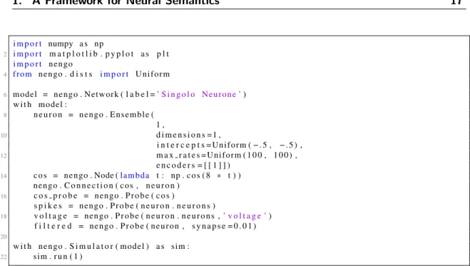
The example shown in this section illustrates how to build and manipulate a single LIF (leaky integrated-and-fire) neuron, which is a standard model of neuron. In this example, a population of neurons formed by a single element is managed. The Figure 1 1.1 shows the Python code of our example. As a first step the neural model (line 6) is created, which represents our simple network and inside which the population of neurons is inserted. A group of neurons is identified in Nengo by an Ensemble object. In our case, when the Ensemble object is created (line 8), the number of neurons it contains is specified (line 9), its size (in our case it is a simple scalar value) and various other parameters that define the characteristics of reaction to the signal.
i m p o r t numpy a s np 2 i m p o r t m a t p l o t l i b . p y p l o t a s p l t i m p o r t n e n g o 4 f r o m n e n g o . d i s t s i m p o r t U n i f o r m 6 model = n e n g o . Network ( l a b e l =’ S i n g o l o N e u r o n e ’) w i t h model : 8 n e u r o n = n e n g o . E n s e m b l e ( 1 , 10 d i m e n s i o n s = 1 , i n t e r c e p t s = U n i f o r m ( − . 5 , − . 5 ) , 12 m a x r a t e s = U n i f o r m ( 1 0 0 , 1 0 0 ) , e n c o d e r s = [ [ 1 ] ] ) 14 c o s = n e n g o . Node (l a m b d a t : np . c o s ( 8 * t ) ) n e n g o . C o n n e c t i o n ( c o s , n e u r o n ) 16 c o s p r o b e = n e n g o . P r o b e ( c o s ) s p i k e s = n e n g o . P r o b e ( n e u r o n . n e u r o n s ) 18 v o l t a g e = n e n g o . P r o b e ( n e u r o n . n e u r o n s ,’ v o l t a g e ’) f i l t e r e d = n e n g o . P r o b e ( n e u r o n , s y n a p s e = 0 . 0 1 ) 20 w i t h n e n g o . S i m u l a t o r ( model ) a s sim : 22 sim . r u n ( 1 )
Figure 1.1: Python code for a single neuron
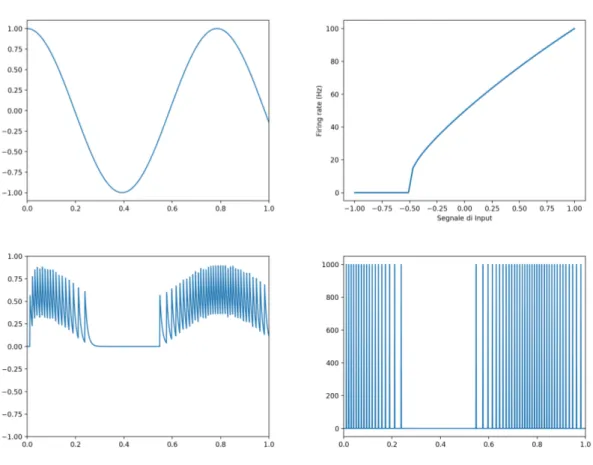
In particular, the neuron is excited by increasing values of the input signal, and this is indicated by the value of encoders set at 1 in line 13. Furthermore, the neuron is excited for signal values higher than -0.5, as indicated in line 11. Finally the maximum value of the signal produced by the neuron is set at 100Hz, as indicated in line 12. In Fig. 1.2 (top right) the tuning curve of the neuron is shown. Notice how the curve assumes values of 0 when the input signal is below the value -0.5. The neuron begins to generate impulses, gradually increasing, starting from the value -0.5 to reach the maximum value (100 Hz) when the input signal reaches the value 1. This curve represents the response of the neuron to the input signal and is independent of the simulation. After defining the characteristics of our neuron, with the help of a Node object, an input signal is simulated, represented by the cosine function λ (t) = cos(8t) (line 14). The Input signal is connected to the population of our network (formed by a single neuron) through a Connection object (line 15). Fig. 1.2 shows (at the top left) the input signal generated in the time span of one second, i.e. for t = 0, . . . , 1. In the subsequent lines of code (lines 16-19), through the Probe objects, data for display and analysis are collected. Finally, in line 21, a Simulator object is created to manage the simulation of our model. This simulation is started for the
Figure 1.2: (Upper left) the input signal identified by the function λ (t) = cos(8t), per t = 0, . . . , 1; (Top right) the tuning curve of the neuron; (Bottom left) the response of the neuron to the stimulus produced by the input signal; (Bottom right) the impulses produced by the single neuron, filtered through a 10ms post-synaptic filter.
duration of a second in line 22 [27].
In Fig. 1.2 (below) are shown the results of the simulation performed on our network. In particular, on the left, the response of the neuron to the stimulus generated by the input signal is represented. Notice how the neuron begins to emit pulses when the input signal is above the −0.5 value. On the right are the impulses produced by the single neuron, filtered through a 10ms post-synaptic filter.
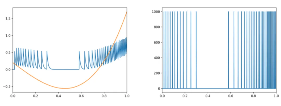
In Fig. 1.3 are shown the results of the simulation performed on the same neural network, considering an input signal linked to the mathematic function λ (t) = 4t3−52t+
1
5. In particular, on the left, is represented the response of the neuron (in blue) to the
Figure 1.3: The results of the simulation performed on a neural network formed from a single neuron, considering an input signal linked to the mathematic function λ (t) = 4t3−52t+15. On the left, the response of the neuron 25 is represented (in blue) to the stimulus generated by the input signal (in orange). On the right are the impulses produced by the single neuron, filtered through a 10ms post-synaptic filter.
by the single neuron, filtered through a 10ms post-synaptic filter.
1.3.2
Representation with a pair of neurons
In this example we show how to create a neural network formed by a pair of neurons with a complementary behavior. As in the previous example, the neurons that form the network are LIF neurons and their behavior is characterized in such a way that one undergoes complementary stimuli to the other. Specifically, the first neuron will increase its spike frequency in response to positive signals, while the latter will increase its spike frequency in response to negative signals. This is the simplest population formed by a pair of neurons capable of providing a reasonable representation of a scalar value.
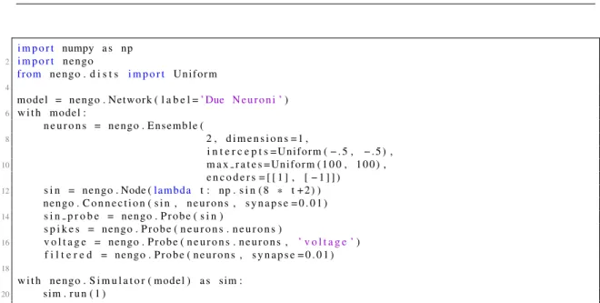
Fig. 1.4 shows the Python code used to manage a couple of neurons. As done in our previous example, we used a Node object for the simulation of the input signal, repre-sented by the cosine function λ (t) = sin(8t + 2) (line 12). The Input signal is connected to the population of our network (formed by a pair of neurons) through a Connection object (line 13).
The population of neurons (defined in line 7) is characterized by a pair of neurons (line 8) whose maximum spike value is equal to 100 Hz (line 10). However, the two
neu-i m p o r t numpy a s np
2 i m p o r t n e n g o
f r o m n e n g o . d i s t s i m p o r t U n i f o r m
4
model = n e n g o . Network ( l a b e l =’ Due N e u r o n i ’)
6 w i t h model : n e u r o n s = n e n g o . E n s e m b l e ( 8 2 , d i m e n s i o n s = 1 , i n t e r c e p t s = U n i f o r m ( − . 5 , − . 5 ) , 10 m a x r a t e s = U n i f o r m ( 1 0 0 , 1 0 0 ) , e n c o d e r s = [ [ 1 ] , [ − 1 ] ] ) 12 s i n = n e n g o . Node (l a m b d a t : np . s i n ( 8 * t +2) ) n e n g o . C o n n e c t i o n ( s i n , n e u r o n s , s y n a p s e = 0 . 0 1 ) 14 s i n p r o b e = n e n g o . P r o b e ( s i n ) s p i k e s = n e n g o . P r o b e ( n e u r o n s . n e u r o n s ) 16 v o l t a g e = n e n g o . P r o b e ( n e u r o n s . n e u r o n s , ’ v o l t a g e ’) f i l t e r e d = n e n g o . P r o b e ( n e u r o n s , s y n a p s e = 0 . 0 1 ) 18 w i t h n e n g o . S i m u l a t o r ( model ) a s sim : 20 sim . r u n ( 1 )
Figure 1.4: Python code for the management of a pair of neurons
rons have a complementary behavior defined by the line 11 encoders: the first neuron is stimulated for increasing values of the input signal, while the second neuron is stimulated for decreasing values. Consequently, since their lower stimulation limit is, for both, equal to −0.5 (line 9), the first neuron will start responding to stimuli for values of the input signal above −0.5, while the second neuron will begin to respond to stimuli for input sig-nal values lower than 0.5. This behavior is highlighted by the graph in Fig 1.5 (top right) in which the tuning curves of the two neurons are shown.
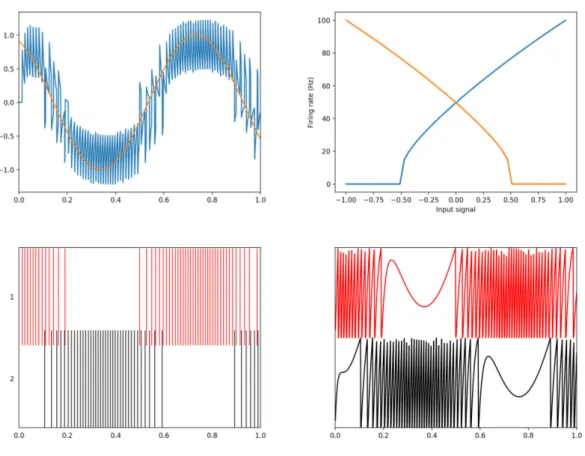
In Figure 51.5 also shows the results of the simulation performed, for a total time of one second, on the neural network just described, formed by a pair of neurons. Specifi-cally, at the top left is the response of the neurons (in blue) to the stimulus generated by the input signal (in orange). In the lower left corner are the impulses produced by the pair of neurons, filtered through a 10ms post-synaptic filter, while the lower right side shows the response of the neurons to the input signal stimuli.
It can be observed how the first neuron is stimulated for values of the input signal between −0.5 and 1, with a spike frequency that gradually increases as the input signal approaches the value 1. In a complementary way the second neuron is stimulated for input signal values between 0.5 and -1, with a spike frequency gradually increasing as
Figure 1.5: The results of the simulation performed, for a total time of one second, on the neural network just described, formed by a pair of neurons. Specifically, at the top left is the response of the neurons (in blue) to the stimulus generated by the input signal (in orange). In the lower left corner are the impulses produced by the pair of neurons, filtered through a 10ms post-synaptic filter, while the lower right side shows the response of the neurons to the input signal stimuli.
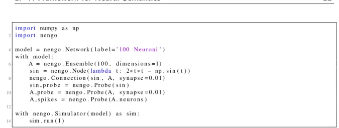
i m p o r t numpy a s np 2 i m p o r t n e n g o 4 model = n e n g o . Network ( l a b e l =’ 100 N e u r o n i ’) w i t h model : 6 A = n e n g o . E n s e m b l e ( 1 0 0 , d i m e n s i o n s = 1 ) s i n = n e n g o . Node (l a m b d a t : 2* t * t − np . s i n ( t ) ) 8 n e n g o . C o n n e c t i o n ( s i n , A , s y n a p s e = 0 . 0 1 ) s i n p r o b e = n e n g o . P r o b e ( s i n ) 10 A p r o b e = n e n g o . P r o b e ( A , s y n a p s e = 0 . 0 1 ) A s p i k e s = n e n g o . P r o b e (A . n e u r o n s ) 12 w i t h n e n g o . S i m u l a t o r ( model ) a s sim : 14 sim . r u n ( 1 )
Figure 1.6: Python code for the management of a pair of neurons
the input signal decreases approaching the value −1. The response of the two neurons to the stimuli provided by the input signal can well represent the input signal in response to which they are activated. We will see in the next sections how the increase in the number of neurons in the population the representation of the input signal will be significantly more accurate.
1.3.3
Representation with a Neural Population
In this example we show how to generate a simple neural network consisting of a popu-lation of 100 neurons. As in previous cases, the popupopu-lation consists of LIF-type neurons whose response properties to the input signal are defined randomly.[51]
La Fig. 1.6 The figure 6 shows the Python code used to manage this population of neurons. As in previous cases, a Node object is used for the simulation of the input signal, represented by the cosine function λ (t) = 2t2− sin(t) (line 7). The population of 100 neurons is created in line 6. The absence of the parameters that define the properties of response to the input signal, indicates that these are generated randomly. The input signal is then connected to the population of our network (formed by a pair of neurons) through a Connection object (line 8). In Figure 1.7 it is shown the graphs related to the tuning curves (on the left) of the 100 neurons that make up the population, and the curve that represents the input signal supplied to the population of neurons (on the right). Notice how the direction of stimulation response, the maximum spike value, and the lower limit
Figure 1.7: The graphs related to the tuning curves (on the left) of the 100 neurons that make up the population, and the curve that represents the input signal supplied to the population of neurons (on the right). (Below) The impulses produced by the population of neurons (on the left), filtered through a post-synaptic filter of 10ms and (on the right) the response of the neurons to the stimulus generated by the input signal.
at which each individual neuron responds are significantly different.
In Figura 1.7 (below) are instead shown the graphs of the results of the simulation performed, for a total time of one second, on the neural network just described. Specifi-cally on the left are the impulses produced by the population of neurons, filtered through a 10ms post-synaptic filter. On the right is the neuron response to the stimulus generated by the input signal.
It can be observed that the accuracy in the representation of the input signal is very good for this population of neurons. This can be evidenced by the fact that the input signal and the output signal generated by the neurons are very similar.
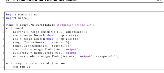
i m p o r t numpy a s np 2 i m p o r t n e n g o 4 model = n e n g o . Network ( l a b e l =’ R e p p r e s e n t a z i o n e 2D ’) w i t h model : 6 n e u r o n s = n e n g o . E n s e m b l e ( 1 0 0 , d i m e n s i o n s = 2 ) s i n = n e n g o . Node (l a m b d a t : np . s i n ( t ) ) 8 c o s = n e n g o . Node (l a m b d a t : np . c o s ( t ) ) n e n g o . C o n n e c t i o n ( s i n , n e u r o n s [ 0 ] ) 10 n e n g o . C o n n e c t i o n ( c o s , n e u r o n s [ 1 ] ) s i n p r o b e = n e n g o . P r o b e ( s i n , ’ o u t p u t ’) 12 c o s p r o b e = n e n g o . P r o b e ( c o s , ’ o u t p u t ’) n e u r o n s p r o b e = n e n g o . P r o b e ( n e u r o n s , ’ o u t p u t ’, s y n a p s e = 0 . 0 1 ) 14 w i t h n e n g o . S i m u l a t o r ( model ) a s sim : 16 sim . r u n ( 5 )
Figure 1.8: Python code for managing a population of 100 neurons
1.3.4
Representation of a pair of signals
In this section we will construct a simple neural network which is able to reacting to an external 2-dimensional signal. In Nengo, this type of signal is managed by a pair of vectors (ie sequences of real values) mono-dimensional. The neural network uses two input communication channels within the same population of neurons.
La Fig. 1.8 shows the Python code used for the simulation of this neural network. The neural model provides for the presence of only one group of neurons, created through a single Ensemble object, calledneurons of 100 neurons (line 6). La specifica dimesione=2 indicates that the neuron population is able to manage two distinct input channels. Two Node objects are used for the simulation of the two input signals which, in our example, are represented by the two sine and cosine functions, ie λ1(t) = sin(t) e λ2= cos(t) (lines
7-8). The two input signals are then connected to the ensemble object through the use of two Connection objects (lines 9-10). However, note that the first signal is connected to the first component of the Ensemble object (neurons[1]) while the second signal is connected to the second component of the Ensemble object (neurons[2]).
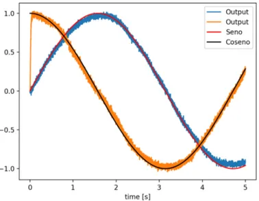
In Figure 1.9 it is shown the graph of the simulation result performed, for a total time of 5 seconds, on the neural network just described. The two outputs produced in response to the two input signals are represented in blue and orange, respectively. Notice how the two signals are faithfully reproduced from the synaptic response of the neuron population.
Figure 1.9: The graph of the simulation result performed, for a total time of 5 seconds, on the neural network just described. The two outputs produced in response to the two input signals are represented in blue and orange, respectively. Notice how the two signals are faithfully reproduced from the synaptic response of the neuron population.
1.3.5
Representation of the sum of two signals
When two input signals converge in the same population of neurons, they combine each other to generate a single signal whose values are given by the sum of the values present in the two original signals. This property is also valid when the two input signals come from the output of two different populations of neurons that react to some external stim-ulus [138].
In this section we will construct a simple neural network capable of simulating the addition of its input signals. The neural network uses two communication channels within the same population of neurons. In this way the addition of the two inout channels is a result that is obtained automatically, since the signals coming from different synaptic connections interact linearly.
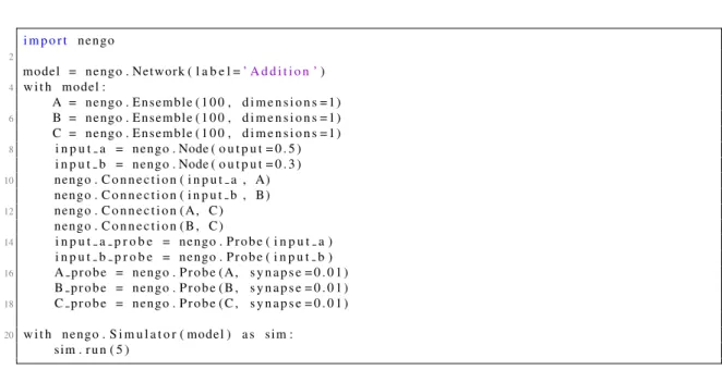
In Figure 1.10 it is shown the Python code used for the simulation of this neural net-work. The neural model provides for the presence of three groups of neurons, created through three Ensemble objects, A, B e C, of 100 neurons each (lines 5-7). Two Node
i m p o r t n e n g o 2 model = n e n g o . Network ( l a b e l =’ A d d i t i o n ’) 4 w i t h model : A = n e n g o . E n s e m b l e ( 1 0 0 , d i m e n s i o n s = 1 ) 6 B = n e n g o . E n s e m b l e ( 1 0 0 , d i m e n s i o n s = 1 ) C = n e n g o . E n s e m b l e ( 1 0 0 , d i m e n s i o n s = 1 ) 8 i n p u t a = n e n g o . Node ( o u t p u t = 0 . 5 ) i n p u t b = n e n g o . Node ( o u t p u t = 0 . 3 ) 10 n e n g o . C o n n e c t i o n ( i n p u t a , A) n e n g o . C o n n e c t i o n ( i n p u t b , B ) 12 n e n g o . C o n n e c t i o n ( A , C ) n e n g o . C o n n e c t i o n ( B , C ) 14 i n p u t a p r o b e = n e n g o . P r o b e ( i n p u t a ) i n p u t b p r o b e = n e n g o . P r o b e ( i n p u t b ) 16 A p r o b e = n e n g o . P r o b e ( A , s y n a p s e = 0 . 0 1 ) B p r o b e = n e n g o . P r o b e ( B , s y n a p s e = 0 . 0 1 ) 18 C p r o b e = n e n g o . P r o b e ( C , s y n a p s e = 0 . 0 1 ) 20 w i t h n e n g o . S i m u l a t o r ( model ) a s sim : sim . r u n ( 5 )
Figure 1.10: Python code for managing a population of 100 neurons
objects are used to simulate the two input signals which, in this example, are represented by the two constant functions λ1(t) = 0.5 e λ2= 0.3 (lines 8-9). The two input signals
are then connected to the A and B populations, respectively, through the use of two Con-nection objects (lines 10-11).
The linear combination of the signals produced in response from the A and B popu-lations is realized by channeling these rials as stimuli for the C population, through the creation of two parallel connections that drive the signal from the two A and B popula-tions. B to the C population (lines 12-13).
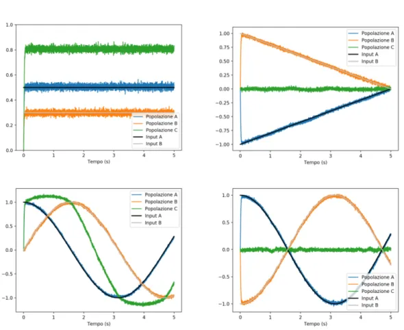
In Figure 1.11 (upper left) it is shown the graphs of the input signals produced by the two Node objects and the results of the simulation performed, for a total time of 5 seconds, on the neural network just described. The synaptic response of the A population is indicated in blue, whereas the population of the B population is orange, while the synaptic response of the C population is indicated in green. It can be seen that the signals coming out of the two populations A and B, faithfully representing the two functions produced by the input signals, converge simultaneously as input of the B population. As a consequence, the latter group of neurons faithfully reproduces the sum of the two signals, producing the desired output in response.
Figure 1.11: The graphs of the simulation performed on a neural network able to repre-sent the sum of two distinct input signals. Specifically, the sum functions of two distinct input signals are represented. Specifically, the functions are represented, λ1(t) = 0.5 and
λ2(t) = 0.3 (in alto a sinistra), λ1(t) = sin(t) and λ2(t) = cos(t) (lower left), λ1(t) = sin(t)
1 i m p o r t numpy a s np i m p o r t n e n g o 3 model = n e n g o . Network ( l a b e l =’ S q u a r i n g ’) 5 w i t h model : A = n e n g o . E n s e m b l e ( 1 0 0 , d i m e n s i o n s = 1 ) 7 B = n e n g o . E n s e m b l e ( 1 0 0 , d i m e n s i o n s = 1 ) s i n = n e n g o . Node (l a m b d a t : 0 . 5 * np . s i n ( t ) ) 9 n e n g o . C o n n e c t i o n ( s i n , A) d e f ampl ( x ) : r e t u r n x [ 0 ] * 2 11 n e n g o . C o n n e c t i o n ( A , B , f u n c t i o n = ampl ) s i n p r o b e = n e n g o . P r o b e ( s i n ) 13 A p r o b e = n e n g o . P r o b e ( A , s y n a p s e = 0 . 0 1 ) B p r o b e = n e n g o . P r o b e ( B , s y n a p s e = 0 . 0 1 ) 15 w i t h n e n g o . S i m u l a t o r ( model ) a s sim : 17 sim . r u n ( 2 0 )
Figure 1.12: Python code for managing a population of 100 neurons
In Figure 1.11 it is also shown the result of the same simulation, performed on three different neural networks in which the input signals introduced in the A and B populations have been changed. Specifically we tested the functions λ1(t) = 1 −15tand λ2(t) =15t− 1
(top right), λ1(t) = sin(t) e λ2(t) = cos(t) (lower left), λ1(t) = sin(t) and λ2(t) = − sin(t)
(lower right). In all cases it is possible to notice how the output signal produced by the B population faithfully reproduces the sum of the two input signals.
1.4
The Transformation Principle with Nengo
In this section I will present some examples of application of the transformation principle in Nengo.
1.4.1
An amplification channel
As seen in the previous examples, a population of neurons can emit an output in response to a signal external to the network, produced by a Node object, or in response to a signal inside the network, produced by one or more populations of neurons [138]. In the previous section, for example, a neural network was created in which a population of neurons emitted a signal in response to the stimulations produced by two different populations of neurons, thus producing a signal that represented the sum of these stimulations.
In this first example of transformation, we show how a population of neurons can be used, not only to represent faithfully or to combine the input received from other popu-lations within the network, but is also able to apply simple linear transformations to the signal of input received. To this end we will create a neural network capable of amplifying the signal received from the outside.
In Figure 1.12 it is shown the Python code used for the simulation of this neural net-work. The neural model predicts the presence of two groups of neurons, created through three Ensemble objects, A and B, of 100 neurons each (lines 6-7). An Node object is used for the simulation of the input signal which, in our example, is represented by the functionλ (t) = 0.5 sin(t) (line 8). The input signal is then connected to the A populations through the use of a Connection object (line 9).
To realize the transformation of the signal it is essential to act on the connection re-alized between the population A and the population B. Specifically, we define a Python function called ampl, which amplifies the signal by doubling the input value. We set ampl(x) = 2x (line 10).
Then a connection is defined between the A population and the B population (line 11) in which the function ampl it is used as a signal filter. This allows the output signal from the Ensemble A object to arrive in the Ensemble B object, with a double intensity.
La Fig. 1.13 shows the graph relating to the simulation performed on the neural net-work just described for a total time of 20 seconds. In blue the signal produced by the population of neurons A is shown, which faithfully reproduces the external input signal, while in orange the output signal produced by the population of B neurons is shown, whose value amplifies that produced by A.
The transformation made in this example can be modified to involve any function on the input signal. For example in Fig. 1.13 (on the right) the 20-second simulation graph is shown on a neural network very similar to the one described in this section, where the transformation function is defined by f (x) = x2. Notice how the signal produced by the Bpopulation (in orange) is actually the square of the output signal generated by the first population of neurons (in blue).
Figure 1.13: The graph relating to the simulation performed on the neural network which carries out an amplification of the signal (on the left) is the square of the signal (on the right). In blue the signal produced by the population is shown that faithfully reproduces the external input signal, while in orange the output signal produced by the transformation is shown.
1.4.2
Arithmetic operations
In this section we will show how, through the transformation of the signal, it is possible to implement arithmetic operations such as multiplying two values. The model that imple-ments this type of transformation can be thought of as a combination of the model used for the representation of a pair of signals and the one used for the representation of the square of a signal, shown in the previous section.
The model (whose code is shown in Fig. 1.14) is composed of four populations of neurons, two of which (called A and B) are used for the representation of external input signals, the third (called combined) it is used for the two-dimensional combination of the two input signals, while the fourth population (called D) is used for the non-linear transformation of the two input signals.
Once again, two Node objects are used for the simulation of the input signal that, in our example, are represented by broken functions defined through the Python model picewise (linee 13-14). I segnali di input vengono poi collegati alle popolazioni A e B, rispettivamente, attraverso l’utilizzo di due oggetti Connection (lines 16-17).
The population combined in line 10, it is defined as a population of two-dimensional neurons. The connection between the A and B populations and the two components of the
1 i m p o r t numpy a s np i m p o r t n e n g o 3 f r o m n e n g o . d i s t s i m p o r t C h o i c e f r o m n e n g o . u t i l s . f u n c t i o n s i m p o r t p i e c e w i s e 5 model = n e n g o . Network ( l a b e l =’ M u l t i p l i c a t i o n ’) 7 w i t h model : A = n e n g o . E n s e m b l e ( 1 0 0 , d i m e n s i o n s = 1 , r a d i u s = 1 0 ) 9 B = n e n g o . E n s e m b l e ( 1 0 0 , d i m e n s i o n s = 1 , r a d i u s = 1 0 ) c o m b i n e d = n e n g o . E n s e m b l e ( 2 2 0 , d i m e n s i o n s = 2 , r a d i u s = 1 5 ) 11 p r o d = n e n g o . E n s e m b l e ( 1 0 0 , d i m e n s i o n s = 1 , r a d i u s = 2 0 ) c o m b i n e d . e n c o d e r s = C h o i c e ( [ [ 1 , 1 ] , [ − 1 , 1 ] , [ 1 , − 1 ] , [ − 1 , − 1 ] ] ) 13 i n p u t A = n e n g o . Node ( p i e c e w i s e ( { 0 : 0 , 2 . 5 : 1 0 , 4 : −10}) ) i n p u t B = n e n g o . Node ( p i e c e w i s e ( { 0 : 1 0 , 1 . 5 : 2 , 3 : 0 , 4 . 5 : 2 } ) ) 15 c o r r e c t = p i e c e w i s e ( { 0 : 0 , 1 . 5 : 0 , 2 . 5 : 2 0 , 3 : 0 , 4 : 0 , 4 . 5 : −20}) n e n g o . C o n n e c t i o n ( i n p u t A , A) 17 n e n g o . C o n n e c t i o n ( i n p u t B , B ) n e n g o . C o n n e c t i o n ( A , c o m b i n e d [ 0 ] ) 19 n e n g o . C o n n e c t i o n ( B , c o m b i n e d [ 1 ] ) d e f p r o d u c t ( x ) : r e t u r n x [ 0 ] * x [ 1 ] 21 n e n g o . C o n n e c t i o n ( combined , p r o d , f u n c t i o n = p r o d u c t ) i n p u t A p r o b e = n e n g o . P r o b e ( i n p u t A ) 23 i n p u t B p r o b e = n e n g o . P r o b e ( i n p u t B ) A p r o b e = n e n g o . P r o b e ( A , s y n a p s e = 0 . 0 1 ) 25 B p r o b e = n e n g o . P r o b e ( B , s y n a p s e = 0 . 0 1 ) c o m b i n e d p r o b e = n e n g o . P r o b e ( combined , s y n a p s e = 0 . 0 1 ) 27 p r o d p r o b e = n e n g o . P r o b e ( p r o d , s y n a p s e = 0 . 0 1 ) 29 w i t h n e n g o . S i m u l a t o r ( model ) a s sim : sim . r u n ( 5 )
Figure 1.15: The graph relating to the simulation carried out on the neural network that produces the product of two signals (on the left), ie the transformation f (x, y) = xy, and the arithmetic transformation f (x, y) = 12x− 2y (on the right). In both cases x and y they represent the two input signals.
combined is carried out on lines 18-19.
Finally, a Python function called product, which has the task of calculating the prod-uct of the two components of the signal x received in input (line 20), and a connection is made between the population combined and the D population, conveyed by the transfor-mation defined by the function product.
In Fig. 1.15 (on the left) shows the graph of the signals generated during the simula-tion produced by our example, with a total durasimula-tion of 5 seconds. The graph shows the representation of the two input signals (in blue and orange, respectively) and the signal produced in response by the D population. Note how this signal is sufficiently close to the function (represented in black) that identifies the actual product between the two input signals.
La Fig. 1.15 (on the right) shows instead the graph of the signals generated during the simulation produced on a neural network that implements the arithmetic transformation f (x, y) =
1
2x− 2y, in which x and y they represent the two input signals. Also in this case the graph
shows the representation of the two input signals (in blue and orange, respectively) and the signal produced in response by the population that applies the non-linear transformation.
i m p o r t n e n g o 2 f r o m n e n g o . u t i l s . f u n c t i o n s i m p o r t p i e c e w i s e 4 model = n e n g o . Network ( l a b e l =’ I n t e g r a t o r e ’) w i t h model : 6 A = n e n g o . E n s e m b l e ( 1 0 0 , d i m e n s i o n s = 1 ) i n p u t = n e n g o . Node ( p i e c e w i s e ( { 0 : 0 , 0 . 2 : 1 , 1 : 0 , 2 : −2 , 3 : 0 , 4 : 1 , 5 : 0 } ) ) 8 t a u = 0 . 1 n e n g o . C o n n e c t i o n ( A , A , t r a n s f o r m = [ [ 1 ] ] , s y n a p s e = t a u ) 10 n e n g o . C o n n e c t i o n (i n p u t, A , t r a n s f o r m = [ [ t a u ] ] , s y n a p s e = t a u ) i n p u t p r o b e = n e n g o . P r o b e (i n p u t) 12 A p r o b e = n e n g o . P r o b e ( A , s y n a p s e = 0 . 0 1 ) 14 w i t h n e n g o . S i m u l a t o r ( model ) a s sim : sim . r u n ( 6 )
Figure 1.16: Codice Python per la gestione di una popolazione di 100 neuroni
1.5
Dynamic Transformations with Nengo
In this section we will show some examples of application of the principle of dynamic transformation in Nengo.
1.5.1
Simulation of a integrator
In mathematics integration is the process that determines the integral of a function, also called quadrature. The integrator is therefore a tool that can determine the integral of a function. The neural model presented in this section implements a mono-dimensional neural integrator, ie an instrument capable of determining the integral of a function ob-tained as an input signal.
This example shows how a population of neurons can be used for the implementation of stable processes of dynamic transformation. These dynamic transformations are at the basis of the implementation of memories, noise cancellation, statistical inference, and many other neural processes.
The model (whose code is shown in Fig. 1.16) it is composed of only one population of neurons, called A, and defined as a group of 100 neurons (line 6). An Node object is used for the simulation of the input signal that, in our example, for simplicity is repre-sented by a broken function defined through the Python model picewise (line 7). The input signal is then connected to the A population through the use of a Connection object
Figure 1.17: The graphs produced by the simulation (of 6 seconds) of a neural model that implements an integrator.
(line 10).
Instead, dynamic transformation is implemented through the creation of a neural con-nection between the A population and itself (line 9). This requires that the output signal generated by the group of neurons, under the stimulus of the input signal, is added to the latter generating a second input which, therefore, varies dynamically over time.
After launching the model simulation for a period of 6 seconds, the graphs is shown in Fig. 1.17 (on the left). Specifically, the input signal is shown in blue, while the output signal produced in response to the stimulation of the neurons is shown in black. Observe how, from the moment the input signal takes on a positive value, the output signal grows steadily. Vice versa, when the input signal takes on a negative value, the output signal decreases proportionally. In the time intervals in which the input signal takes the value 0, the integrator assumes instead maintains its constant value, as it is logical to expect. In Fig. 1.17 (on the right) the graph of the output signal produced by the same neural model is also shown under the stimulus of a different input function.
Because the integrator was built through a neural model, it does not behave perfectly. By running the simulation several times it is possible to highlight the errors produced by the model. These errors can be significantly reduced by increasing the number of neurons in the population.
2
The Semantic Pointer Architecture
This chapter details the cognitive architecture called Semantic Pointer Architecture (SPA). Like any cognitive architecture, SPA represents only a hypothesis of how concepts are represented in our neural system and of the functioning of cognitive processes that lead to intelligent behaviors [129].
2.1
The semantic pointer
At the basis of the SPA is the hypothesis of the existence of semantic pointers. The pur-pose of introducing this hypothesis is to bridge the gap between the neural structure used in the NEF, based on the idea that a wide variety of functions can be implemented in neural structures, and the domain of cognition (which needs ideas on how such neural structures give rise to complex behaviors). In SPA, the syntax is inspired by supporters of the symbolic approach who argue for the presence of syntactically structured representa-tions in the head, while the semantics is inspired by connectionists who argue that vector spaces can be used to capture important semantic features .
2.1.1
Physical characterization of a semantic pointer
Semantic pointersare a means of linking more general neurological representations (sym-bols) to the central ones of cognition. They can be generated from raw perceptual inputs or can be used, for example, to guide a motor action. Specifically, according to this hypothesis, higher-level cognitive functions in biological systems are made possible by such pointers. Such pointers are neural representations that carry a partial semantic con-tent and are composable in the representational structures necessary to support a more complex process of cognition.
2.1.2
Mathematical characterization of a semantic pointer
A semantic pointer is mathematically characterized as a vector of dimension n, that is, as an element of a vector space n -dimensional. A n -dimensional vector is made up of a sequence of n numeric values, called components of the vector.
For example, the sequence (2, 6, 3) represents a vector in the vector space at 3 di-mension; the sequence (2, −4, 0) represents a vector in a space of 2 didi-mension; while (6, 1, 2, −3, −8) represents a vector in vector space at 5 dimension.
To understand what a vector is and how it can be represented graphically, let’s consider the 2 dimensional vector space (n = 2) represented by the Cartesian plane, very familiar to us. In Fig. 2.1 (on the left) the Cartesian plane is shown in which three vectors are highlighted. They are graphically represented as segments starting from the origin (the point (0, 0)) and ending in the point (x, y), characteristic of each vector. Each vector in the 2 dimension plan is therefore uniquely defined by its 2 components: x and y. The three vectors represented in Fig. 2.1 (on the left) are the vectors (2, 2), (−2, 3) and (−4, 1). In a 3 dimension vector space, like the one shown in Fig. 2.1 (right) each vector is defined by a set of 3 numbers (x, y, z). The vector represented in the figure is defined by the triple (5, 8, 3).
A high-dimensional vector space is a natural way of representing semantic relation-ships in a cognitive system. Although it is difficult to visualize high-dimensional spaces, we can understand how this statement can work in the representation of concepts in a three-dimensional space (a relatively low-dimensional space). We refer to this