A
A
l
l
m
m
a
a
M
M
a
a
t
t
e
e
r
r
S
S
t
t
u
u
d
d
i
i
o
o
r
r
u
u
m
m
–
–
U
U
n
n
i
i
v
v
e
e
r
r
s
s
i
i
t
t
à
à
d
d
i
i
B
B
o
o
l
l
o
o
g
g
n
n
a
a
DOTTORATO DI RICERCA IN
Ingegneria Biomedica, Elettrica e dei Sistemi
Ciclo 33°
Settore Concorsuale: 09/E4
Settore Scientifico Disciplinare: ING-INF/07
TITOLO TESI
Design and Implementation of New Measurement Models and
Procedures for Characterization and Diagnosis of Electrical Assets
Presentata da:
Abbas Ghaderi
Coordinatore Dottorato
Supervisore
Prof. Michele Monaci
Prof. Lorenzo Peretto
Abstract
The measurement is an essential procedure in power networks for both network stability, and diagnosis purposes. This work is an effort to confront the challenges in power networks using metrological approach. In this work three different research projects are carried out on Medium Voltage underground cable joints diagnosis, inductive Current Transformers modeling, and frequency modeling of the Low power Voltage Transformer as an example of measurement units in power networks. For the cable joints, the causes and effects of Loss Factor has been analyzed, while for the inductive current transformers a measurement model is developed for prediction of the ratio and phase error. Moreover, a frequency modeling approach has been introduced and tested on low power voltage transformers. The performance of the model on prediction of the low power voltage transformer output has been simulated and validated by experimental tests performed in the lab.
Keywords: Measurement Setup, Power Network, Cable Joint, Current Transformer, Low Power
i
Contents
1 Introduction ...1
2 Power systems and measurement ...3
2.1 Instrument Transformers in Power Systems ...5
2.1.1 Inductive CTs and VTs in power networks ...6
2.1.2 Low Power Instrument Transformers ...8
2.2 Measurement for diagnosis in power systems ...10
3 Definitions in Metrology ...11
3.1 Metrology and Measurement ...11
3.2 Uncertainty in Measurement ...13 3.3 Calibration ...13 3.4 Calibration Hierarchy ...14 3.5 Verification ...14 3.6 Validation ...15 3.7 Metrological Traceability ...15 3.8 Calibration Process ...15
3.8.1 Instrument Transformers Calibration ...16
3.8.2 Instrument Transformer Calibration using Calibrator Devices ...17
3.8.3 Measurement setup calibration ...18
4 Measurement for MV Cable Joints Diagnosis ...19
4.1 Test Setup Design, and Calibration for Tan Delta Measurements on MV Cable Joints ...20
4.1.1 Cable joint description ...20
4.1.2 Test Setup Design ...21
4.1.3 Sample Preparation ...23
4.1.4 Tan Delta Measurement Technique ...24
4.1.5 Tan Delta Measurement Results ...28
4.1.6 Conclusions ...29
4.2 Effects of Temperature on MV Cable Joints Tan Delta Measurements ...29
4.2.1 Sample Preparation ...29
4.2.2 Measurement Procedure ...30
4.2.3 Measurement Results ...31
ii
4.3 Effects of Mechanical Pressure on the Tangent Delta of MV Cable Joints ...35
4.3.1 Test Setup Description ...35
4.3.2 Test procedure ...36
4.3.3 Test Results ...38
4.3.4 Conclusions ...39
4.4 Test Bed Characterization for the Interfacial Pressure vs. Thermal cycle Measurements in MV Cable Joints ...40
4.4.1 Measurement Setup ...41
4.4.2 Description of the Experimental Tests ...46
4.4.3 Results and Discussion ...47
4.4.4 Conclusion ...51
5 Measurement Model for Inductive Current Transformers ...53
5.1 Inductive Current Transformer Core Parameters Behaviour vs. Temperature Under Different Working Conditions...53
5.1.1 Test Setup ...54
5.1.2 Experimental Tests Procedure ...55
5.1.3 Tests Results ...58
5.1.4 Conclusions ...61
5.2 Procedure for Inductive Current Transformers error prediction at Different Operating Conditions ...61
5.2.1 Test Setup ...62
5.2.2 Experimental Tests and Analysis...63
5.2.3 Experimental tests and accuracy prediction results ...66
5.2.4 Conclusions ...70
6 Low-Power Voltage Transformer Smart Frequency Modeling and Output Prediction up to 2.5 kHz, Using Sinc-Response Approach ...71
6.1 LPVT Model ...72
6.2 IR Test Method vs. SR Test Method ...74
6.2.1 IR Test Method ...74
6.2.2 SR Test Method ...75
6.3 Sinc Signal Design ...76
6.3.1 Sinc Function Fourier-Transform Analysis ...77
6.3.2 Sinc Function Characteristic ...78
6.3.3 Sinc Function Fourier Series Coefficients ...79
6.4 Experimental Test Setup ...80
6.5 Experimental Tests ...81
iii
6.5.2 SF Test Procedure ...82
6.5.3 DW Test Procedure ...82
6.5.4 Output Prediction and Validation ...82
6.6 Results ...85
6.6.1 SR Experimental Test Results ...85
6.6.2 Transfer Functions ...87
6.6.3 SF Experimental Test Results ...89
6.6.4 DW Experimental Test Results ...90
6.6.5 Output Prediction and Validation ...91
6.7 Conclusion ...94
7 Conclusions ...95
iv
LISTOFFIGURES
FIGURE 2-1.FROM LEFT TO RIGHT:MVINDUCTIVE CURRENT TRANSFORMER FOR INDOOR APPLICATION,HV OIL -PAPER INSULATION INDUCTIVE CURRENT TRANSFORMER FOR OUTDOOR APPLICATION, HV COMBINED
CURRENT AND VOLTAGE TRANSFORMER ...7
FIGURE 2-2.FROM LEFT TO RIGHT:MVINDUCTIVE VOLTAGE TRANSFORMER FOR INDOOR APPLICATION,HV OIL -PAPER INSULATION VOLTAGE TRANSFORMER FOR OUTDOOR APPLICATION, HV CAPACITIVE VOLTAGE TRANSFORMER ...8
FIGURE 2-3.FROM LEFT TO RIGHT: SPLIT CORE ROGOWSKI COIL LPCT,UNIFORM CORE ROGOWSKI COIL LPCT, MVCOMBINED LPIT FOR INDOOR APPLICATION,MVCOMBINED LPIT FOR OUTDOOR APPLICATION ...9
FIGURE 2-4.FROM LEFT TO RIGHT:MVCAPACITIVE LPVT FOR OUTDOOR APPLICATION,MVCAPACITIVE LPVT FOR INDOOR APPLICATION,MVRESISTIVE LPVT ...10
FIGURE 3-1.ITCALIBRATION TEST SETUP USING A TRACEABLE REFERENCE IT TO BE COMPARED WITH THE IT UNDER CALIBRATION ...17
FIGURE 3-2.ITCALIBRATION TEST SETUP USING A TRACEABLE REFERENCE SIGNAL CALIBRATOR AND WITHOUT REFERENCE IT AND COMPARATOR ...18
FIGURE 4-1.CABLE JOINT CROSS SECTION DESCRIPTION (COURTESY OF REPLITALY) ...20
FIGURE 4-2.AUTOMATIC MEASUREMENT SETUP FOR THE TAN DELTA MEASUREMENT ...22
FIGURE 4-3.EQUIVALENT ELECTRIC CIRCUIT OF THE PROPOSED SETUP ...22
FIGURE 4-4.PICTURE OF THE CABLE JOINT UNDER TEST BEFORE AND AFTER ITS PREPARATION WITH ALUMINIUM FOILS ...23
FIGURE 4-5.PICTURE FROM THE CABLE:1, THE LONGEST INSULATOR PATH CONSIDERED,2 AND 3 THE MINIMUM INSULATOR PATH USED FOR SURFACE DISCHARGE TEST ...24
FIGURE 4-6. RIGHT: EQUIVALENT CIRCUIT OF A CABLE JOINT LEFT: DISSIPATION ANGLE REPRESENTED IN THE PHASORS PLANE ...24
FIGURE 4-7.TAN DELTA MEASUREMENT ALGORITHM ...27
FIGURE 4-8.VOLTAGE AND CURRENT PHASORS ACQUIRED FOR THE TAN DELTA MEASUREMENT ...28
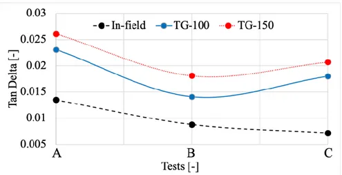
FIGURE 4-9.TAN DELTA VS. TEMPERATURE MEASUREMENT RESULTS FOR THE IN-FIELD CABLE JOINT ...32
FIGURE 4-10.TAN DELTA VS. TEMPERATURE MEASUREMENT RESULTS FOR THE TG100 CABLE JOINT ...33
FIGURE 4-11.TAN DELTA VS. TEMPERATURE MEASUREMENT RESULTS FOR THE TG150 CABLE JOINT ...33
FIGURE 4-12.TAN DELTA VS. TEMPERATURE MEASUREMENT RESULTS FOR THE 3 CABLE JOINTS UNDER TEST AT 60°C ...34
FIGURE 4-13.PICTURE OF THE HOSE CLAMP USED TO APPLY PRESSURE TO THE CABLE JOINT UNDER TEST ...36
v
FIGURE 4-15.ELECTRIC POTENTIAL DISTRIBUTION AND ELECTRIC FIELD COMPONENTS OF A SIMULATED CABLE
JOINT ...37
FIGURE 4-16.SCHEMATIC REPRESENTATION OF THE PRESSURE APPLICATION AND MEASUREMENT ...38
FIGURE 4-17.TAN DELTA MEASUREMENT RESULTS FOR ALL THE THREE PRESSURE TESTS ...39
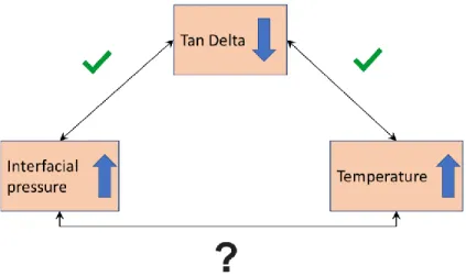
FIGURE 4-18. CAUSE AND EFFECT LOOP FOR THE RELATION BETWEEN TAN DELTA, TEMPERATURE, AND INTERFACIAL PRESSURE IN CABLE JOINTS ...40
FIGURE 4-19.SCHEMATIC OF THE MEASUREMENT SETUP AND PRESSURE SENSORS POSITIONING ...42
FIGURE 4-20.CABLE JOINT STRUCTURE WITH PARTICULAR ATTENTION TO THE PARTS OF INTEREST ...43
FIGURE 4-21.PICTURE OF THE ADOPTED PRESSURE SENSOR ...45
FIGURE 4-22.TEMPERATURE VS. DURATION OF THE TESTS ON THE CUTS ...47
FIGURE 4-23.POSITIONING OF THE TWO SENSORS INSIDE THE CUT AND OF THE CUT ITSELF...49
FIGURE 4-24.PRESSURE MEASUREMENT RESULTS FOR CUTA, SENSORS 𝐴1 AND 𝐴2 ...49
FIGURE 4-25.PRESSURE MEASUREMENT RESULTS FOR CUTB, SENSORS 𝐵1 AND 𝐵2 ...49
FIGURE 4-26. CAUSE AND EFFECT LOOP FOR THE RELATION BETWEEN TAN DELTA, TEMPERATURE, AND INTERFACIAL PRESSURE IN CABLE JOINTS ...52
FIGURE 5-1.CIRCUIT DIAGRAM OF THE MEASUREMENT SETUP ADOPTED FOR THE TESTS ...55
FIGURE 5-2.CIRCUIT DIAGRAM OF THE MEASUREMENT SETUP ADOPTED FOR THE SHORT CIRCUIT TESTS ...56
FIGURE 5-3.CIRCUIT DIAGRAM OF THE MEASUREMENT SETUP ADOPTED FOR THE OPEN CIRCUIT TESTS ...57
FIGURE 5-4.CIRCUIT DIAGRAM OF THE CT EQUIVALENT CIRCUIT CONSIDERED ...58
FIGURE 5-5.SHUNT PARAMETERS REPRESENTATION VS. TEMPERATURE VS. APPLIED VOLTAGE ...61
FIGURE 5-6.MEASUREMENT SETUP ADOPTED FOR THE RATED CONDITIONS TESTS ...63
FIGURE 5-7.PART OF THE CT EQUIVALENT CIRCUIT DETAILING THE SHUNT PARAMETERS AND THE BURDEN ...64
FIGURE 5-8.COMPLETE MODEL OF THE CT ADOPTED IN THE WORK...64
FIGURE 5-9.FUNCTIONS 𝑒𝑇 AND 𝑒𝐶 FOR THE RATIO ERROR PREDICTION ...69
FIGURE 5-10.FUNCTIONS 𝑓𝑇 AND 𝑓𝐶 FOR THE PHASE DISPLACEMENT PREDICTION ...69
FIGURE 6-1.LOW-POWER VOLTAGE TRANSFORMERS (LPVT) ELECTRIC EQUIVALENT CIRCUIT ...73
FIGURE 6-2.DESIGNED NORMALIZED SINC SIGNAL.(A)TIME DOMAIN;(B) DISCRETE FOURIER TRANSFORM (DFT) MAGNITUDE ...76
FIGURE 6-3.SAMPLING PRINCIPLE OF AN ARBITRARY SIGNAL ...78
FIGURE 6-4.ECPERIMENTAL TEST SETUP SCHEME ...80
FIGURE 6-5. (A)DFT MAGNITUDE OF THE INPUT SINC SIGNAL; (B) DFT MAGNITUDE OF THE SINC-RESPONSE SIGNAL;(C) RATIO BETWEEN DFT MAGNITUDE OF INPUT SINC AND SINC-RESPONSE SIGNAL ...84
vi
FIGURE 6-6.REFERENCE INPUT SINC SIGNAL APPLIED TO THE LPVT UNDER TEST, MEASURED BY REFERENCE RESISTIVE–CAPACITIVE VOLTAGE DIVIDER AND THE INPUT SINC SIGNAL MEASURED BY THE LPVT UNDER TEST (LPVT SINC-RESPONSE TRANSFERRED TO THE PRIMARY SIDE) ...86 FIGURE 6-7.RATIO ERROR TREND VS. FREQUENCY ...86 FIGURE 6-8.PHASE DISPLACEMENT TREND VS. FREQUENCY ...87 FIGURE 6-9.TIME DOMAIN UNFILTERED VERSION OF THE LPVT SAMPLED DATA TRANSFER FUNCTION.(A) ALL 10,000 SAMPLES;(B) FIRST 9 SAMPLES;(C) ONLY THE FIRST SAMPLE REMOVED;(D) SAMPLES FROM THE 2ND TO THE 50TH. ...88 FIGURE 6-10.TIME DOMAIN FILTERED VERSION OF THE LPVT SAMPLED DATA TRANSFER FUNCTION. (A) ALL 10,000 SAMPLES;(B) FIRST 9 SAMPLES;(C) ONLY THE FIRST SAMPLE REMOVED;(D) SAMPLES FROM THE 2ND TO THE 50TH. ...89 FIGURE 6-11.SYNTHESIZED SINUSOIDAL INPUT SIGNAL AND THE MEASURED SIGNAL PREDICTION BY SIMULATION.
(A) PREDICTION FOR 50HZ;(B) PREDICTION FOR 500HZ;(C) PREDICTION FOR 1 KHZ. ...92 FIGURE 6-12.SYNTHESIZED DISTORTED INPUT SIGNAL AND THE MEASURED SIGNAL PREDICTION BY SIMULATION.
(A) PREDICTION FOR 1ST +3RD HARMONICS;(B) PREDICTION FOR 1ST +5TH HARMONICS;(C) PREDICTION FOR 1ST +7TH HARMONICS;(D) PREDICTION FOR 1ST +3RD +5TH +7TH HARMONICS. ...93
vii
LISTOFTABLES
TABLE 2-1.LIMITS OF RATIO ERROR AND PHASE DISPLACEMENT FOR MEASURING CURRENT TRANSFORMERS...6
TABLE 2-2.LIMITS OF VOLTAGE ERROR AND PHASE DISPLACEMENT FOR MEASURING VOLTAGE TRANSFORMERS ...6
TABLE 4-1.DETAILED RESISTORS SPECIFICATION ...22
TABLE 4-2.RESULTS OF THE RESISTOR CHARACTERIZATION ...25
TABLE 4-3. THE TAN DELTA MEASUREMENT RESULTS FOR 7 DIFFERENT CABLE JOINTS IN TERMS GLASS TRANSITION TEMPERATURE ...28
TABLE 4-4. CHAUVIN ARNOUX 863DIGITAL THERMOCOUPLE SPECIFICATIONS ...31
TABLE 4-5.TAN DELTA VS.TEMPERATURE MEASUREMENT RESULTS ...32
TABLE 4-6.TAN DELTA VARIATION BETWEEN MINIMUM AND MAXIMUM TEMPERATURE APPLIED TO THE CABLE JOINTS ...33
TABLE 4-7.PRESSURE SENSORS MAIN SPECIFICATIONS ...36
TABLE 4-8.TAN DELTA RESULTS DURING THE PRESSURE TEST FOR THE CABLE JOINTS UNDER TEST ...38
TABLE 4-9.PRESSURE SENSOR MAIN SPECIFICATIONS ...45
TABLE 4-10.LIST OF ALL PRESSURE MEASUREMENT RESULTS FOR THE 2CUTS ...48
TABLE 5-1.NI-9239 MAIN FEATURES ...54
TABLE 5-2.FLUKE 6105A MAIN FEATURES ...55
TABLE 5-3.COMPONENTS CHARACTERIZATION RESULTS ...55
TABLE 5-4.RATED CONDITIONS TEST RESULTS ...58
TABLE 5-5.SHORT CIRCUIT TEST RESULTS FOR DIFFERENT LOAD CURRENTS ...59
TABLE 5-6.CT SERIES PARAMETERS COMPUTATION RESULTS, FOR DIFFERENT LOADS AND TWO TEMPERATURES ...59
TABLE 5-7.OPEN CIRCUIT TEST RESULTS FOR DIFFERENT LOAD CURRENTS ...60
TABLE 5-8.CT SHUNT PARAMETERS COMPUTATION RESULTS, FOR DIFFERENT LOADS AND TWO TEMPERATURES ...60
TABLE 5-9.FLUKE TRANSCONDUCTANCE 52120A MAIN CHARACTERISTICS ...63
TABLE 5-10.CT SHUNT PARAMETERS FOR DIFFERENT LOADS AND TEMPERATURES ...66
TABLE 5-11.RATIO ERROR AND PHASE DISPLACEMENT RESULTS AND THE DECOMPOSITION AT 24°C ...66
TABLE 5-12.RATIO ERROR AND PHASE DISPLACEMENT RESULTS AND THE DECOMPOSITION AT 40°C ...67
TABLE 5-13.RATIO ERROR AND PHASE DISPLACEMENT RESULTS AND THE DECOMPOSITION AT 50°C ...67
TABLE 5-14.RATIO ERROR AND PHASE DISPLACEMENT RESULTS AND DECOMPOSITION AT 65°C ...67
TABLE 5-15.QUASI-IDEAL TRANSFORMER RATIO AND PHASE DISPLACEMENT FOR TEMPERATURES 24°C AND 40 °C ...67
viii
TABLE 5-16.QUASI-IDEAL TRANSFORMER RATIO AND PHASE DISPLACEMENT FOR TEMPERATURES 50°C AND 65
°C ...67
TABLE 5-17.DYNAMIC COEFFICIENTS AND THEIR FUNCTIONS ...69
TABLE 6-1.TREK POWER AMPLIFIER FEATURES ...81
TABLE 6-2.EXPERIMENTAL SR TEST RESULTS IN TERMS OF 𝜀 AND ∆Φ. ...85
TABLE 6-3.EXPERIMENTAL SF TEST RESULTS ...90
TABLE 6-4.EXPERIMENTAL DW TEST RESULTS. ...90
TABLE 6-5.SFPREDICTION RESULTS AND COMPARISON WITH SR EXPERIMENTAL TEST RESULTS ...92
ix
Acronyms
MV Medium Voltage IT Instrument Transformer CT Current Transformer VT Voltage TransformerLPIT Low Power Instrument Transformer
LPCT Low Power Current Transformer
LPVT Low Power Voltage Transformer
SE State Estimation
EMS Energy Management System
PMU Phasor Measurement Units
CIT Combined Instrument Transformer
CVT Capacitive Voltage Transformer
HV High Voltage
DG Distributed Generation
PD Partial Discharge
DUT Device Under Test
VIM International Vocabulary of Metrology
GUM Guide to the Expression of Uncertainty in Measurement
ADC Analog to Digital Convertor
THD Total Harmonic Distortion
DSO Distribution System Operator
DAQ Data Acquisition Board
TG Glass Transition Temperature
CUT Cable joint Under Test
DN Distribution Network
TUT Transformer Under Test
SC Short Circuit FT Fourier Transform OC Open Circuit RC Rated Condition AC Accuracy Class IR Impulse Response SR Sinc Response
DFT Discreet Furies Transform
DTFT Discrete Time Fourier Transform
FS Fourier Series
SF Single Frequency
DW Distorted Waveform
IS Input Sinc
1
1 Introduction
The metrology processes are ongoing in our everyday life and have a more professional role in engineering and industries as well. For the engineering purposes, measurement instruments are used widely. The mass-produced devices which are used as measurement instruments, are already designed, and implemented for specific tasks. The user can use them without being concerned about the measurement processes which are handled inside the instrument. As the measurement instruments are developed for specific tasks and challenges in different fields of engineering, it is always probable to require a measurement unit which has not been developed before as a massed-produced unit. In this case, the prototype measurement setup needs to be developed and implemented. Moreover, sometimes the economical convenience is the reason to design and develop the prototype measurement setup in the lab for specific purposes. In case of design and implementation of measurement setup prototypes, it is not a plug and play instrument as mass produced measurement instrument. In this case the knowledge of metrology is required to accurate development of such setup. Here is the importance of measurement field of study in deeper sense.
This work is an attempt to use metrology and measurement science to develop measurement test setups for the power networks purposes. In detail, 3 different works are performed on power networks with the metrology point of view: i) test setup has been developed for Medium Voltage (MV) cable joints diagnosis in power network. ii) a measurement model has been developed for inductive Current Transformer (CT) modeling. iii) the test setup is developed with new system identification method (Sinc Response approach) for the Low Power Voltage Transformers frequency modeling.
The theoretical studies, experimental tests, analysis, and the results are part of the 3-year Ph.D. research work which are resulted in 14 scientific paper publication in prestigious journals, conferences, workshops, and scientific symposiums. Regarding the time frame, some research works were continuously ongoing for three years. For example, MV cable joint diagnosis is composed of few different and time-consuming tests that it is required to spend few months for cable joints material relaxation after each set of tests. On the other hand, other projects were planned for specific time period to take advantage of the whole three years.
2
The present Ph.D. thesis is structured as 8 chapters which are described as following: section 2 introduces the role of measurement in power systems and crucial role of measurement for the power networks stability. The voltage and frequency control and their link to the voltage, current, and phase measurement is highlighted. Furthermore, the concept of State Estimation (SE) is introduced to emphasize the importance of measurement accuracy on estimation of the current and voltage at power network nodes which are not equipped with measurement units.
Section 3 establishes the main definitions in metrology which are used during this research work. Moreover, the concept of calibration is highlighted by definition and introducing the adopted test setups for calibration. Different alternatives are described specifically for calibration of instruments. Furthermore, the calibration and characterization concept of measurement units are extended to the measurement setup. It means that the calibration and characterization of the measurement setup is distinguished compared to the measurement units.
In section 4 the Tan Delta measurement setup is developed for MV cable joint diagnosis. The implemented setup is used to analyze the Tan Delta of underground cable joints vs temperature. In next step, the relation between Tan Delta in cable joints vs interfacial pressure between cable and joint common surface, has been analyzed. At the last step in MV cable joint diagnosis, a test setup is designed and implemented to measure the interfacial pressure in cable joints and analyzing the pressure variation vs. thermal cycles applied to the cable joint.
Section 5 deals with the inductive Current Transformers modeling and core parameters extraction using a designed measurement setup. After the core parameter extraction, their variation vs temperature and their effect on CT accuracy is studied. Afterward, the CT is considered as an RL filter and the measured ratio and phase errors are decomposed to extract the effect of only filtering behavior on the CT accuracy. Using the same data, dynamic calibration coefficients are calculated to compensate the CT ratio and phase error under different temperatures and different loading conditions.
Section 6 concerns a new approach introduced as Sinc Response approach for Low Power Voltage Transformer (LPVT) frequency modeling up to 2.5 kHz. The normalized Sinc signal is designed and analyzed for transfer function extraction and prediction of the LPVT output for any known input signals with frequency harmonics less than 2.5 kHz.
In Section 7 some conclusions are stated, and section 8 presents the main references and published paper during the 3-years research work.
3
2 Power systems and measurement
The measurement can affect power systems mostly in two different ways. One for the technical necessity for accurate voltage and current measurement by measurement unit calibration and characterization, and the other for a more general requirement for power network components diagnostic methods based on measurement. The technical necessity concerns the power network state variables measurement for load flow studies and power network control for stability reason. The more general requirement concerns the measurements for apparatus diagnosis or performing tests on power system components.
Accurate measurement of electrical quantities in power systems is getting more and more a challenging subject for many reasons. With moving from traditional to modernized power systems and networks new concepts, such as electricity market and Smart Grids introduce more and more challenges to overcome. As well known, electric power is considered as a product to be sold in a competitive market. Hence the exact amount of bought or sold electric power should be known with a necessary and required accuracy.
Moreover, from a technical point of view, the measurement of voltages and currents at each node of the power network is required in order to perform a correct voltage and frequency control, and to assure an optimum power flow. Stability of power system, reactive power compensation and fault detection are also directly dependent on these measurements.
The procedure adopted to manage the network control is to inject the measured quantities into a State Estimators (SE). A SE is an algorithm running in the control room processing system whose output is the estimated value of power network state variables (voltages, currents, and phase) in all the nodes with or without measurement units. A SE allows also to estimate quantities at those nodes of the network which are not equipped with measurement units. A modern Energy Management System (EMS) collects in real-time all remote measured quantities from the nodes and provides the solution of the network as its output for fast and live power flow analysis, control, fault location, etc. State estimation is based on mathematical relations between state variables of the system and measured values. In particular, state variables of a typical power network are the currents and the amplitude of the voltages at each bus along with the phase displacement of voltage phasors with respect to the reference universal time. In such
4
dynamic systems, there is usually a minimum number of state variables to be measured for attaining the full observability of the whole network.
The most important challenge in state estimation is that the measured information, remotely taken and transmitted to the control unit, must feature high accuracy. Moreover, the communication infrastructure must feature suitable reliability.
In order to overcome the aforementioned challenges, measurements need to be first traceable. This is performed by checking and monitoring the metrological confirmation of the measuring units. The metrological confirmation is a set of operations required to ensure that measuring equipment conforms to the requirements for its intended use. Metrological confirmation generally includes calibration and verification. Measurement units technologically are of different type: simple power meters in a given power network node or modern Phasor Measurement Units (PMU).
As mentioned, stability enhancement and fast and robust control of a power network can be reached by measuring phasors of voltage and current at each node and bus or the network and by comparing the phase displacement of the voltage phasors with respect to a reference universal time. One of the important issues to tackle is that the measurement instrumentation is not present in all nodes of distribution networks. This is mainly due by economic as well as practical reasons. So, the accurate estimation of the state variables is accomplished as soon as the measurements in those nodes equipped with measurement units is performed with high accuracy. There are in literature many methods and algorithms capable to reconstruct the measurements at the nodes not covered by instrumentation. The evaluation of the state variables by means of a partial coverage of measuring devices in the networks can be performed by using probabilistic as well as deterministic approaches. They make use of the measurements in the monitored nodes to estimate the measurements in all blind ones. In general, the main limit of all such approaches is that they suffer consistently by the measurement errors. Such errors arise from the non-complete coverage of measurements in network nodes and from the instrumentation used. The combination of such errors can lead to unreliable and very inaccurate evaluation of state variables and, in turn, to a wrong control of the power flow in the network.
Still today there are uncontrollable differences between estimated values of quantities in nodes not equipped with instrument devices and measurements performed in the same nodes by portable measurement instrumentation used for comparison. The main sources of errors are noise added to measured quantities, instrument errors, time difference between measured values, incorrect information about topology of the network, etc. In literature studies aimed at providing information on the sources of errors and how to deal with them in state estimation can be found [1] [2] [3].
5
The error detection and identification in measurements is one of the most important attributes of the state estimation process in power systems. Some research can be found in literature also in this area. However, at present, error detection and identification is mainly done under the assumption that only one source of error is affecting the measurement results. To reduce the State Estimator output error, at least we need to provide as accurate as possible measurements in the nodes equipped with the measurement units.
The most widespread measurement units are the Instruments Transformers (IT) which are divided to Current Transformers (CT), and Voltage Transformers (VT) categories to measure the current and voltage, respectively. In case of High voltage measurements, Capacitive Voltage Transforms (CVT) are deployed. The Combined Instrument Transformers (CIT) are equipped with both CT and VT in a single unit. The new generation of instrument transformers are more efficient in their size, weight, and the frequency band. The new generation of instrument transformers known as Low Power Instrument Transformers (LPIT) are designed to measure both current and voltages. Low Power Current transformers (LPIT), and Low Power Voltage Transformers (LPVT) are the terminology referring to the LPITs used for current and voltage measurement, respectively.
The calibration and characterization of instrument transformers to reduce the measurement error is the main role of measurement in power networks. On the other hand, to ensure good performance of power system components such as cable joints and terminations, power transformers, switches, etc., diagnostic methods based on measurement are used. This is the second role of measurement for power networks.
2.1 Instrument Transformers in Power Systems
As referred before, Instrument Transformers are used to perform current and voltage measurements in power network nodes. The ITs are the most widespread measurement units deployed in power networks. In general, the ITs use for two purposes: for protection and for measurement.
The ITs used for protection purpose, are not required to have high measurement accuracy. The the main challenge related to protection ITs concerns detection of voltages and currents much higher than rated ones. The detected high current or voltage, triggers the related protection relays for saving the feeder and avoiding damage to the network. In protection CTs, the saturation of magnetic core is challenging, while in protection VTs insulation and withstand is the challenge which is considered during the design.
6
The ITs used for measurement purposes are the set of ITs which concern the present work. Measurement ITs should hold their promised accuracy class as they are used for power network control and for billing purposes. The accuracy of ITs is evaluated by reporting the ratio error and phase error or phase displacement as two indicative parameters for ITs performance. The accuracy class of measurement ITs is declared on the nameplate and each accuracy class indicates the allowed ratio and phase error. The standard bodies provide the accuracy classes and related ratio and phase errors for each accuracy class. Table 2-1 and Table 2-2 present the accuracy classes for CTs and VTs, respectively from standards [4], and [5].
Table 2-1. Limits of ratio error and phase displacement for measuring current transformers
Accuracy class
Ratio error [± %] Phase displacement
at current [% of rated] ± Minutes ± Centiradians at current [% of rated] at current [% of rated] 1 5 20 50 100 120 1 5 20 100 120 1 5 20 100 120 0.1 - 0.4 0.2 - 0.1 0.1 - 15 8 5 5 - 0.45 0.24 0.15 0.15 0.2 - 0.75 0.35 - 0.2 0.2 - 30 15 10 10 - 0.9 0.45 0.3 0.3 0.5 - 1.5 0.75 - 0.5 0.5 - 90 45 30 30 - 2.7 1.35 0.9 0.9 1 - 3.0 1.5 - 1.0 1.0 - 180 90 60 60 - 5.4 2.7 1.8 1.8 0.2s 0.75 0.75 0.75 0.75 0.75 0.75 30 30 30 30 30 0.9 0.9 0.9 0.9 0.9 0.5s 1.5 1.5 1.5 1.5 1.5 1.5 90 90 90 90 90 2.7 2.7 2.7 2.7 2.7 3 - - - 3 - 3 - - - - 5 - - - 5 - 5 - - - -
Table 2-2. Limits of voltage error and phase displacement for measuring voltage transformers
Accuracy class
Ratio error [± %] Phase displacement
± Minutes ± Centiradians 0.1 0.1 5 0.15 0.2 0.2 10 0.3 0.5 0.5 20 0.6 1.0 1.0 40 1.2 3.0 3.0 - -
2.1.1 Inductive CTs and VTs in power networks
The traditional current and voltage transformers which are the most historical measurement unites used in AC power networks, are based on inductive current and voltage transformation. These type of
7
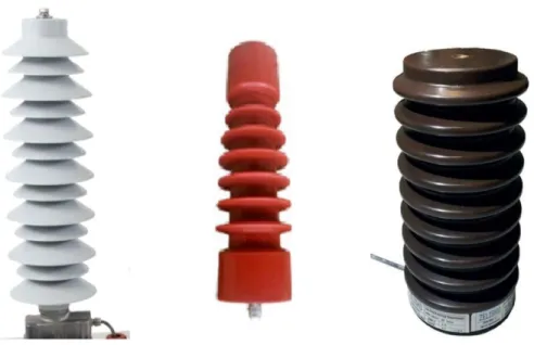
Figure 2-1. From left to right: MV Inductive Current Transformer for indoor application, HV oil-paper insulation Inductive Current Transformer for outdoor application, HV Combined Current and Voltage Transformer
ITs are designed for High Voltage (HV), and Medium Voltage (MV) levels for both indoor and outdoor applications. Therefore, they are mostly installed in high voltage and distribution substations.
As they are designed based on magnetic induction, the primary and secondary windings in addition to insulation system makes the size and weight considerable which is suitable to be installed in substations. With smart grids point of view, it is required to have CTs and VTs with smaller size and lighter weight to measure the current and voltage Distributed Generation (DG) nodes. In this case using big and heavy inductive ITs is challenging.
The other challenge to use inductive ITs in smart grid environment for DG measurement is the bandwidth which is related to power quality measurement. By increasing use of power electronic components in power networks (in power converters, electric drives, active rectifier, active filters etc.), and high frequency harmonics injection in the network, measurement units should measure the current and voltages up to 2.5 kHz which is power quality frequency range. Inductive ITs especially inductive CTs are limited in frequency range. The inductive ITs behavior in low frequency range or for DC component measurement is not applicable due to inductive law principles. Moreover, nowadays by growing electrical technologies there are quite wide range of applications with current and voltage frequencies much more different than power networks (50 Hz, and 60 Hz) which are required to be measured (such as electric trains). Figure 2-1 and Figure 2-2 show some types of well-known inductive CTs and combined ITs, and VTs in power networks, respectively.
8
Figure 2-2. From left to right: MV Inductive Voltage Transformer for indoor application, HV oil-paper insulation Voltage Transformer for outdoor application, HV Capacitive Voltage Transformer
Aforementioned facts are the motivation for invention of new instrument transformers with higher weight, smaller size and more bandwidth called Low Power Instrument Transformers (LPIT).
2.1.2 Low Power Instrument Transformers
Low Power Instrument transformers are referred to Low Power Current Transformers (LPCT) and Low Power Voltage Transformers (LPVT) for current and voltage measurement solution, respectively. Unlike the inductive CT and VT, LPCTs and LPVTs are based on different principles.
2.1.2.1 Low Power Current Transformers
As inductive CTs, the LPCTs are based on magnetic induction, but using Rogowski coil magnetic material which has low magnetic permeability and close to air. Using high reluctance magnetic core leads to measuring high current with small output signal in the range of milliampere. The small output magnitude implies the concept of low power terminology. The output signal can be available in both current and voltage solutions. The LPCTs can be designed with both uniform core and split core magnetic material. During manufacturing process, the magnetic core can be shielded for immunity versus electric or magnetic fields. Figure 2-3 shows some samples of more used LPCTs and combined LPITs.
9
Figure 2-3. From left to right: split core Rogowski coil LPCT, Uniform core Rogowski coil LPCT, MV Combined LPIT for indoor application, MV Combined LPIT for outdoor application
The LPCTs based on Rogowski coil not only measure accurately a high range of alternating current, but also have a wide frequency range up to few kHz. The different types of LPCTs are also used in application diverse than power network like Partial Discharge (PD) measurement of HV cables for cable diagnostics.
2.1.2.2 Low Power Voltage Transformers
Contrary to inductive VTs which are based on magnetic induction, the LPVTs are based on voltage dividers. The technology can be found based on capacitive, resistive, and resistive capacitive voltage divider. Figure 2-4 represents different types of LPVTs for MV power networks. The resistive LPVTs are easier in terms of implementation but they are vulnerable to electric fields and if it is not well shielded, the ratio and phase error is affected by influence quantities especially electric field. For this reason, capacitive LPVTs are more efficient compared to the other aforementioned types.
On the other hand, capacitive LPVTs are challenging in terms of implementation as the primary capacitance should extruded during the LPVT manufacturing. LPVTs based on capacitive dividers are mainly designed in active and passive configurations. The difference between the two categories concerns the design limitation and the customer preference.
10
Figure 2-4. From left to right: MV Capacitive LPVT for outdoor application, MV Capacitive LPVT for indoor application, MV Resistive LPVT
Normally, the secondary capacitor is an embedded one, while the primary capacitor is a built-in capacitor obtained from the chassis of the device. For this reason, the built-in primary capacitance may vary from device to device, hence leading to different transformation ratios for different products. To normalize the transformation ratio and phase displacement of each product to the nominal values (after the characterization process) correction factors are provided to the customer by the manufacturer. This type of capacitive LPVTs are the passive ones. It should be noted that in any case the accuracy class is not compromised.
In active LPVTs an active electronic amplifier is added to the passive LPVTs to bring the transformation ratio and phase displacement to the nominal ones so that all final products keep the nominal values declared on the nameplate without introducing extra correction factors.
2.2 Measurement for diagnosis in power systems
In addition to measurement application at power network nodes for control and stability reasons, measurement knowledge is used for diagnosis purposes in power networks. Power networks include a wide range of electric assets, apparatus, and widespread components such as cables, joints, terminations, etc.. The apparatuses such as power transformers, circuit breakers, switchgears, surge arresters, etc. are prone to type tests or routine tests. In order to perform such tests, there is a measurement setup to be designed, calibrated, and implemented. Widespread components such as cables, cable joints, and
11
terminations should be diagnosed to determine their performance. Moreover, test setups can be designed to characterize and calibrate the measurement units in power network.
Two well-known diagnostic methods for cables, cable joints, and terminations are Partial Discharge (PD) measurement and Tan Delta measurement. The two methods can be applied on different samples in the lab environment for further studies to improve their operation or to indicate the state of insulation health. In any case the measurement setups need to be designed, implemented, and calibrated to perform the studies.
In this work, different test setups are designed and implemented for the purpose of MV cable joints, characterization, calibration of inductive CTs, and LPVTs modeling. It should be noted that there are instruments designed by manufacturers to do some the tests, but using the science of metrology, lets us to design a customized version of the setup, which is cheaper, accurate, and reliable. Tests for diagnostic and characterization purposes are normally done in the lab environment, except for some portable test setups designed for the in-field measurements such as portable standard units for online instrument transformers calibration.
3 Definitions in Metrology
Nowadays, measurement instruments affect our life in different ways. In our daily life we read instruments too many times. For example, reading the speed indicator in the car, reading the car, reading the scale in grocery store, etc.. The everyday used measurement instruments perform measurements and provide us with the measurement results for daily life. In a more specified way, we need to understand what measurement is, and which parameters are defined as tools for performing measurements. In this chapter the purpose is to define the concepts related to metrology which are used in following chapters. To this purpose, it is taken advantage of International Vocabulary of Metrology (VIM) referenced in [6] for the definitions and descriptions.
3.1 Metrology and Measurement
Metrology
Metrology is the science of measurement and its application. Metrology includes all theoretical and practical aspects of measurement, whatever the measurement uncertainty and field of application is. In this regard, the measurement should be defined.
12
Measurement
Measurement is the process of experimentally obtaining one or more quantity values that can reasonably be attributed to a quantity. So, a measurement process provides, as a part of the measurement
result, one or more quantity values that can be attributed to a quantity intended to be measured, that is
also called, always according to the VIM [6], measurand [7].
To fully understand this definition, we have to refer to the definition of quantity. We can find it again in the VIM.
Quantity
Property of a phenomenon, body, or substance, where the property has a magnitude that can be expressed as a number and a reference.
The VIM states that a reference can be a measurement unit, a measurement procedure, a reference
material, or a combination of such.
When physical properties are considered, the reference is generally a measurement unit, whilst, when chemical measurement are considered, the reference is quite often a reference material.
The quantity values provided by the measurement are therefore a number and a reference together expressing the magnitude of a quantity [7].
Is this the measurement result? Or, better, can a measurement result be expressed only by a number and a reference? As we will see later in section 1.5 of this chapter, a measurement procedure cannot provide the “true” value of a measurand, due to several factors that we will thoroughly discuss later. This means that a measurement result can only provide a finite amount of information about the measurand, and we must know if that amount is enough for the intended use of the measurement result. Otherwise, the measurement result would be meaningless [7].
Therefore, any measurement result has to be provided with an attribute capable of quantifying how close to the measurand’s value the obtained quantity value is. This attribute is called uncertainty, and the correct definition of measurement result, as provided by the VIM, is as follows [7].
Measurement result
Set of quantity values being attributed to a measurand together with any other available relevant information.
In a note to this general definition, the VIM states that:
A measurement result is generally expressed as a single measured quantity value and a
13
The above general definitions have introduced a number of concepts (quantity value, reference,
relevant information, uncertainty), that will be covered in the next Sections, and show that a
measurement is a definitely more complex procedure than simply reading an instrument.
The science that includes all theoretical and practical aspects of measurement, regardless to the measurement uncertainty and field of application, is called metrology and it is already defined in the present section as “the science of measurement and its application” according to VIM [6].
3.2 Uncertainty in Measurement
The knowledge conveyed by the measurement result is aimed at quantifying how complete the information associated with the quantity values provided by the measurement process is [7].
The problem of qualifying the measurement result with a quantitative attribute capable of characterizing the completeness of the information provided about the measurand has been considered since the beginning of metrology and has undergone a significant revision during the last two decades of the twentieth century, when the modern concept of uncertainty has been introduced and adopted.
Understanding this concept is not immediate. As noted by the Guide to the Expression of Uncertainty in Measurement (GUM) [8], the word uncertainty means doubt, and thus in its broadest sense uncertainty of measurement means doubt about the information provided by the result of a measurement. The first question that we have to answer to, if we wish to fully understand the uncertainty concept, is where this doubt originates and why [7].
However, the concept of doubt is hardly quantifiable. Therefore, the use of the term uncertainty to quantify how much we should doubt about the obtained measurement result seems somehow contradictory and tautological, since we apparently try to quantify a doubt with a doubt!
Fortunately, this contradiction is only apparent and is due to a lexical problem. Because of the lack of different words for the general concept of uncertainty and the specific quantities [7].
3.3 Calibration
Calibration is defined as operation that, under specified conditions, in a first step, establishes a relation between the quantity values with measurement uncertainties provided by measurement
standards and corresponding indications with associated measurement uncertainties, and in a second
step, uses this information to establish a relation for obtaining a measurement result from an indication [6].
14
A calibration may be expressed by a statement, calibration function, calibration diagram,
calibration curve, or calibration table. In some cases, it may consist of an additive or multiplicative correction of the indication with associated measurement uncertainty. Calibration should not be confused
with adjustment of a measuring system, often mistakenly called “self-calibration”, nor with verification of calibration. Often, the first step alone in the above definition is perceived as being calibration [6].
3.4 Calibration Hierarchy
By VIM definition [6], calibration hierarchy is a sequence of calibrations from a reference to the final measuring system, where the outcome of each calibration depends on the outcome of the previous calibration.
Measurement uncertainty necessarily increases along the sequence of calibrations. The elements
of a calibration hierarchy are one or more measurement standards and measuring systems operated according to measurement procedures. For this definition, the ‘reference’ can be a definition of a
measurement unit through its practical realization, or a measurement procedure, or a measurement
standard. A comparison between two measurement standards may be viewed as a calibration if the comparison is used to check and, if necessary, correct the quantity value and measurement uncertainty attributed to one of the measurement standards [6].
3.5 Verification
VIM [6] defines the verification as provision of objective evidence that a given item fulfils specified requirements. An example is the confirmation that performance properties or legal requirements of a measuring system are achieved.
When applicable, measurement uncertainty should be taken into consideration for verification procedure. The item for verification may be a process, measurement procedure, material, compound, or measuring system and the specified requirements may be that a manufacturer's specifications to be met [6].
Verification in legal metrology, in conformity assessment in general, pertains to the examination and marking and/or issuing of a verification certificate for a measuring system. Verification should not be confused with calibration and not every verification is a validation [6].
15
3.6 Validation
Validation is the verification, where the specified requirements are adequate for an intended use [6]. For example, a measurement procedure, ordinarily used for the measurement of Tan Delta of a cable sample, may be validated also for measurement of Tan Delta of cable joint.
3.7 Metrological Traceability
Metrological traceability is the property of a measurement result whereby the result can be related to a reference through a documented unbroken chain of calibrations, each contributing to the
measurement uncertainty . For this definition, a ‘reference’ can be a definition of a measurement unit
through its practical realization, or a measurement procedure including the measurement unit for a
non-ordinal quantity, or a measurement standard [6].
Metrological traceability requires an established calibration hierarchy. Specification of the reference must include the time at which this reference was used in establishing the calibration hierarchy, along with any other relevant metrological information about the reference, such as when the first calibration in the calibration hierarchy was performed [6].
For measurements with more than one input quantity in the measurement model, each of the input
quantity values should itself be metrologically traceable and the calibration hierarchy involved may form
a branched structure or a network. The effort involved in establishing metrological traceability for each input quantity value should be commensurate with its relative contribution to the measurement result [6]. Metrological traceability of a measurement result does not ensure that the measurement uncertainty is adequate for a given purpose or that there is an absence of mistakes. A comparison between two measurement standards may be viewed as a calibration if the comparison is used to check and, if necessary, correct the quantity value and measurement uncertainty attributed to one of the measurement standards. The abbreviated term “traceability” is sometimes used to mean ‘metrological traceability’ as well as other concepts, such as ‘sample traceability’ or ‘document traceability’ or ‘instrument traceability’ or ‘material traceability’, where the history (the “trace”) of an item is meant. Therefore, the full term of “metrological traceability” is preferred if there is any risk of confusion [6].
3.8 Calibration Process
The metrological calibration process in the world of measurement technology is the documented comparison of the measurement device to be calibrated against a traceable reference device. As it is
16
highlighted, the metrological calibration concerns a measurement device. For some measurement devices such as Instrument Transformers, the accuracy class is one of the most important characteristics of that measurement unit. Therefore, if the purpose is to characterize the accuracy class of an instrument transformer, it can be considered as part of the calibration procedure. This is a source of confusion between ITs calibration and characterization, while most of measurement units unlike the ITs get calibrated and not characterized in terms of their accuracy.
In case of other elements which are not measurement devices, the characterization makes a totally independent sense rather than calibration. For example, in case of a Resistor to be characterized, the
resistance value is the main characteristic to be found accurately. As it is clear, the resistance value can
be measured using a measurement unit or measurement setup with a calculated uncertainty. In the Resistor characterization example, a measurement setup for resistor characterization can be composed of a calibrated voltage source, and a calibrated current meter (or a characterized shunt resistor). Both calibrated voltage source and current meter can be traceable reference devices.
The ratio and phase errors are the main characteristics of Instrument Transformers, the ratio and phase errors should be calculated for both characterization and calibration. Namely, based on calibration definition, the process for ITs calibration or characterization is the same as calibration of a general measurement device. For this reason, even for ITs we refer to the term “calibration” rather than “characterization”.
3.8.1 Instrument Transformers Calibration
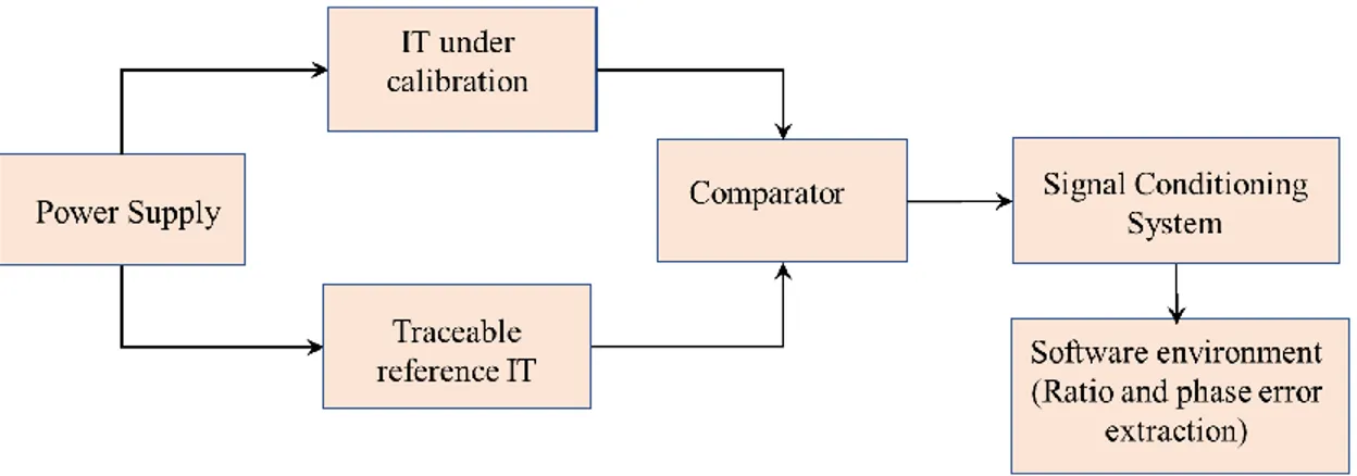
The purpose is to provide the possible procedures for ITs calibration in a measurement lab. As mentioned in previous section, by calibration, the ratio and phase error are extracted as main characteristics of the instrument transformers. The ratio and phase error calculation are used multiple times for studies in next chapters and for this reason the instrument transformers calibration process should be studied. Based on the calibration definition, the ITs calibration procedure requires a measurement setup composed of a traceable reference instrument transformer to be compared with the Device Under Test (DUT) which is the instrument transformer to be calibrated. Figure 3-1 represents such calibration setup.
17
Figure 3-1. IT Calibration test setup using a traceable reference IT to be compared with the IT under calibration
The main components of such calibration setup are: Power supply, traceable reference instrument transformer, comparator, IT under calibration, signal conditioning acquisition system, and a processing unit or a PC to perform the numerical analysis. The signal conditioning system refers to the possible amplifiers or attenuators, Analog to Digital Convertor (ADC), and the rest of data acquisition chain. In case of Electronic ITs, sometimes the primary signal needs to be amplified and it is possible to have more amplifiers in the calibration setup. It should be noted that, in addition to traceable reference IT which is the core of the calibration setup, the comparator and all components of signal conditioning chain have to be characterized and calibrated to have a calibrated calibration setup. It is important to mention that the power supply is not required to be calibrated as long as both reference IT and IT under test experience the same signal in primary side. Regarding the power supply, the Total Harmonic Distortion (THD) of the signal must be negligible and it is necessary to perform Discreet Furies Transform (DFT) analysis to extract the main harmonic.
3.8.2 Instrument Transformer Calibration using Calibrator Devices
The alternative solution for ITs calibration without a traceable IT, is to focus on the power supply side and use a traceable voltage calibrator (in case of VT calibration) or traceable current calibrator (in case of CT calibrator). In this case, the applied voltage or current signals are guaranteed to be accurate and they don’t need to be compared with the signal measured by a traceable reference IT. As a result, this setup does not have neither the reference IT, nor the comparator. The test setup is composed of reference standard signal calibrator, IT under test, signal conditioning system, and the PC for numerical
18
Figure 3-2. IT Calibration test setup using a traceable reference signal calibrator and without reference IT and comparator
analysis. Figure 3-2 shows a schematic of the calibration test setup with reference calibrator and without both reference instrument transformer and comparator.
3.8.3 Measurement setup calibration
Measurement setup are developed and implemented for perform measurement for different purposes. For example, in next chapters a measurement setup has been designed to measure loss factor (Tan Delta) of cable joint, while a measurement setup can be designed to calibrate or characterized in instrument transformer (calibration test setup). In any case, a guarantee is required to have an accurate and reliable measured value. In other word, the measurement setup has to be calibrated by itself. If we consider a calibration setup, even the calibration setup needs to be calibrated by itself.
By calibration definition, the device under calibration should be compared with a reference one. If the setup is a protype implemented in laboratory, this task can be done by characterization or calibration of any single component of the measurement setup under calibration. For example, if there is any amplifier in the measurement setup, it should be characterized separately by another setup, or if there is any comparator, it should be calibrated by a separate calibration setup and the error due to the comparator should be compensated. The term “characterization” is used for the amplifier, because it is considered as a component with a specific transformation ratio and not a measurement unit, while the term “calibration” is used for the comparator as it is a measurement unit which measures the difference between two signals.
19
4 Measurement for MV Cable Joints Diagnosis
The use of underground medium voltage (MV) cables is nowadays widespread among utilities. Its usage allows network operators to avoid all the issues that arise from the deployment of overhead lines and cables. For example, vegetation is one frequent cause of failure for overhead lines. In addition, overhead cables, which seem to protect the power network from that issue, are affected, mainly in the rural areas, by hunters’ bullets. They damage, in multiple points, the typical 3 bundled cables which compose the power network. This results in very difficult-to-detect faults position and expensive cables replacements.
For the abovementioned reasons, underground cables are deployed in many countries. However, they are not fault-free. In particular, the majority of faults happen in the critical points of a cable: the terminals and the joints. Other sources of faults could be related to the cable insulation, but they are frequently due to external causes (mechanical actions on the cable) independent of the electrical characteristics. Considering now the main causes of fault, specific monitoring systems must be implemented to understand why they happen. Scientific literature contains a variety of contributes which could be distinguished, firstly, in on-line [9] and off-line [10] monitoring. Clearly, the former is considerably tougher than the latter due to the limitation of maintaining the network powered.
In this section, the attention is focused on one of the critical causes and components of fault in the cable: the joint. It is fundamental either for enlarging or restoring the power networks when a fault happens. However, the high rate of cable joint explosion causes intensive costs for maintenance, increases the outage time, and penalizes the Distribution System Operators (DSOs) as they cannot deliver the promised electric power. These issues for underground cable power networks make it necessary to study the diagnostic methods to prevent cable joints explosion, hence the outage of the power network. To this purpose, different diagnostic techniques have been developed in the literature. For example, partial discharge (PD) measurement is tackled in [11], while the electric field analysis is described in [12] and [13]. Another paramount diagnostic method, which can provide crucial information about the aging of the joints due to different influent quantities, is the Tangent Delta (or Tan Delta, Tg) measurement. In [14], [15], [16] high frequency tests have been applied on joints to extract Tg, while in-field measurements have been performed in [17] to extract Tg and PD.
In the following, first the test setup has been designed and implemented to measure the Tan Delta related to MV underground cable joints. In the second stage, the Tan Delta variation vs. Temperature has
20
Figure 4-1. Cable joint cross section description (courtesy of REPL Italy)
been tackled. Afterwards, the Tan Delta variation vs. interfacial pressure inside the cable joints has been studied. At the end, to close the cause-and-effect loop, the measurement setup to measure the interfacial pressure inside the cable joint is designed, and interfacial pressure variation vs. temperature is analyzed.
4.1 Test Setup Design, and Calibration for Tan Delta Measurements on MV Cable Joints
In this subsection, a simple test setup to measure Tan Delta of cable joint samples has been designed and calibrated for the purpose of MV underground cable joints diagnosis. The setup is designed and tested under 1 kV applied voltage and 50 Hz frequency.
In the following we will see: description a cable joint in detail, the proposed test setup for the Tan Delta measurement, cable joint preparation in order to being tested with the setup, and then the Tan Delta measurement technique is fully described. The test results are presented afterwards, and finally the conclusions are stated.
4.1.1 Cable joint description
To clarify the aim of this work, a cable joint needs to be fully described. In Figure 4-1 it can be seen all the layers which compose the joint. From the outside to the inside there are:
1. the cold shrink.
2. the metallic mesh, it connects the ground potential between the two portions of cable separated by the joint.
3. the silicon rubber covered by an inner and an outer semi-conductive layer, to uniformize the electric field. Such silicon will be the layer under test for the Tan Delta measurement.
21
Cable joints are installed all along the network to extend it or restore it in case of faults. They connect two pieces of cable which could be, in some cases, either of different insulations (e.g. XLPE cables and paper-oil cables) or of different conductor materials (copper or aluminum). The outer part of a joint, the shrink, complete the joint covering everything on its inside, preventing damages and external actions. This part could be built in two different ways, referred as: cold shrink and heat shrink. The former consists in a silicon material placed over a removable plastic core. When removed, the rubber seals around the conductor. The latter, instead, requires a source of heat, for example from a gas torch, to shrink over the joint. Recently, the cold shrinks are substituting the use of heat shrinks. This is because there is no need of direct flames to install them, hence there is a reduced risk for both the user and the joint itself.
Another paramount component of the joint is the dielectric layer (item 3 in Figure 4-1). It is the insulator, hence representable with a capacitor and a resistor in parallel, that cover the junction created from the union of the two portions of cable. The quality of this layer, can be evaluated with the Tan Delta measurement, detailed in the following, which reveal the dielectric degradation.
4.1.2 Test Setup Design
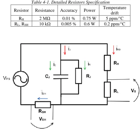
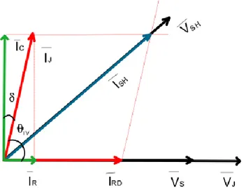
Figure 4-2 shows a schematic representation of the Tan Delta automatic measurement setup. It includes: a programmable power source Agilent 6813B, an isolation transformer, a step-up voltage transformer (0.1 kV/15 kV), a resistive voltage divider, a shunt resistor, a Data Acquisition Board NI9239 (DAq), a personal computer and of course the cable joint under test. The power source is used to provide a 50 Hz-sinusoidal voltage. This way, voltage distortions and frequency changes are avoided, which can lead to an incorrect estimate of the Tan Delta. The power source voltage output, raised through the step-up transformer, feeds the cable joint under test with a voltage limited to 1 kV RMS, for minimizing the risk of joint discharge. The resistive voltage divider is composed by RH = 2 MΩ and RL = 10 kΩ, on the high and low voltage sides, respectively. It is used to measure the voltage 𝑉̅𝐽 at the cable joint terminals, by means of the DAq. The NI9239 Data Acquisition board is used in all my research projects and it features 24-bit ADC resolution, 50 kS/s/ch sample rate, 0.03% gain error, and 0.008% of offset error. The NI9239 Data Acquisition Board uncertainty has been analyzed in section 4.1.4.1.
22
Figure 4-2. Automatic measurement setup for the Tan Delta Measurement
Figure 4-3. Equivalent electric circuit of the proposed setup
To measure the current provided by the step-up transformer, a shunt resistor RSH = 10 kΩ has been used. Its voltage-drop 𝑉̅𝑆𝐻 it is acquired by the DAq. Table 4-1 lists the specifications of RSH, RH and RL. The equivalent circuit of the proposed setup is shown in Figure 4-3. CJ and RJ represent the equivalent capacitance and resistance of the joint under test, respectively. Under working conditions, the power dissipated by the resistors is significantly lower than their rated one, except for RH, where rated and dissipated power are comparable (0.75 W and 0.55 W). However, due to its very lower thermal drift (5 ppm/°C) this does not affect the accuracy.
Table 4-1. Detailed Resistors Specification
Resistor Resistance Accuracy Power Temperature drift RH 2 MΩ 0.01 % 0.75 W 5 ppm/°C
23
Figure 4-4. Picture of the cable joint under test before and after its preparation with aluminium foils
4.1.3 Sample Preparation
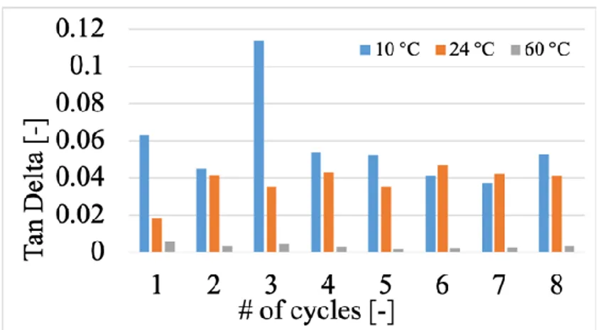
Samples used for Tan Delta measurement are cold shrink joints and the insulating material is silicon rubber. Seven samples are used with Glass Transition Temperature (TG) ranging from 90 °C to 150 °C
with steps of 10 °C. The joints connect two pieces of 130 mm2 cables having length of about 0.5 m. Glass
Transition Temperature of a material is the temperature at which the transition from the glassy to the rubbery state starts. TG is always lower than the melting temperature of the material.
The samples used do not have the outer shrink and the metallic mesh, hence the dielectric object of study is already available. However, to perform a Tan Delta measurement, the metallic mesh is required for being used as ground potential electrode. The high voltage potential electrode is given by the cable conductor. Therefore, an aluminium foil layer has been applied to the dielectric of the joint to recreate the ground electrode. This can be seen in Figure 4-4, where the upper picture represents the original joint while the lower picture the joint after the aluminium application.
As for the contribution of the surface discharge to the Loss Factor, a simple test has been performed. Tan Delta has been measured when the discharge from the conductor to the semiconductor was very long (picture 1 in Figure 4-5) and when it was the shortest possible which is the radius of the cable (picture 2 and 3 of Figure 4-5). The results of both tests were identical; hence the surface discharge effect is negligible and then not considered in the following results.
24
Figure 4-5. Picture from the cable: 1, the longest insulator path considered, 2 and 3 the minimum insulator path used for surface discharge test
Figure 4-6. Right: equivalent circuit of a cable joint Left: dissipation angle represented in the phasors plane
4.1.4 Tan Delta Measurement Technique
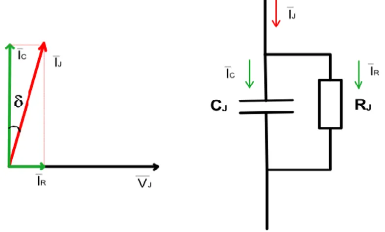
Before detailing the procedure adopted for the measurements, Tan Delta must be defined. Figure 4-6 shows the equivalent circuit of a cable joint. It is then possible to define the Tan Delta (or dissipation factor) as ratio between the current flowing through the joint equivalent resistor and the one flowing through its equivalent capacitor (4-1).
𝑇𝑎𝑛 (𝛿) = 𝐼̅𝑅
𝐼̅𝐶 ( 4-1 )
25
4.1.4.1 RSH, RH and RL calibration
One element required to the Tan Delta measurement setup (Figure 4-2) is the resistive voltage divider. It allows to measure the voltage applied to the cable joint V̅𝐽 and it needs to be characterized. To this purpose, 1000 measurement have been acquired for all the resistors using the multimeter HP 3458A under metrological confirmation. According to [18] it features the following accuracy specification: 10 ppm of reading and 0.5 ppm of range, and 50 ppm of reading and 10 ppm of range, for the 10 kΩ and 10 MΩ ranges, respectively. Table 4-2 lists the mean value, the standard deviation 𝑢𝐴 of the 1000 measurement performed, the standard uncertainty 𝑢𝐵 (obtained from the multimeter parameters) and the relative
combined uncertainty 𝑢𝐶 = √𝑢𝐴2+ 𝑢
𝐵2/𝑅 of the two resistors RL and RH that compose the divider and
the shunt resistor RSH used for the current measurement. It can be noted that all the combined uncertainties
are lower than the rated accuracy provided by the manufacturers (Table 4-1). In addition, from the results of the Table the mean value and the uncertainty affecting the resistive divider ratio have been calculated. It is:
𝐾 = 201.01 ± 0.02 ( 4-2 ) using a coverage factor of 2 and being,
𝐾 =𝑅𝐿+𝑅𝐻
𝑅𝐿 ( 4-3 )
Hence:
𝑉̅𝐽 = 𝐾𝑉̅𝑆 ( 4-4 )
AS Equation (4-4) shows, the uncertainty related to 𝑉̅𝐽 is driven from the uncertainty calculated for 𝐾 (Equation (4-2)) and the uncertainty of measured 𝑉̅𝑆. The systematic contribution to uncertainty of NI9239 Data Acquisition Board can give quantitative value for uncertainty to be sure that it can be neglected. To this purpose, we know that the cable joint experiences 1kV test voltage (|𝑉̅𝐽|) and considering the transformation ratio of the resistive voltage divider (𝐾 = 200), we have 5V in the resistive divider output (|𝑉̅𝑆|). Given that the NI9239 DAQ features 0.03% gain error and 0.008% of full-scale
Table 4-2. Results of the Resistor Characterization
Resistors Mean Value [Ω] 𝑢𝐴 [ Ω] 𝑢𝐵 [ Ω] 𝑢𝐶 [-]
RH 2.0000∙106 30 115 5.9∙10-5
RL 9.9999∙103 0.005 0.06 6.0∙10-6