UNIVERSITÀ CATTOLICA DEL SACRO CUORE
Dipartimento di Economia e Finanza
Working Paper Series
Public Expenditure Multipliers in recessions.
Evidence from the Eurozone
Andrea Boitani and Salvatore Perdichizzi
Working Paper n. 68
March 2018
Public Expenditure Multipliers in recessions.
Evidence from the Eurozone
Andrea Boitani
Università Cattolica del Sacro Cuore
Salvatore Perdichizzi
Università degli Studi di Bologna
Working Paper n. 68
March 2018
Dipartimento di Economia e Finanza Università Cattolica del Sacro Cuore Largo Gemelli 1 - 20123 Milano – Italy tel: +39.02.7234.2976 - fax: +39.02.7234.2781
e-mail: [email protected]
The Working Paper Series promotes the circulation of research results produced by the members and affiliates of the Dipartimento di Economia e Finanza, with the aim of encouraging their dissemination and discussion. Results may be in a preliminary or advanced stage. The Dipartimento di Economia e Finanza is part of the Dipartimenti e Istituti di Scienze Economiche (DISCE) of the Università Cattolica del Sacro Cuore.
Public Expenditure Multipliers in recessions.
Evidence from the Eurozone
Andrea Boitani∗, Salvatore Perdichizzi†
22nd March 2018
Abstract
During the sovereign debt crisis, many Euro countries have deployed “austerity packages” implementing structural reforms and cutting government spending. Such policies should have led to an initial decline in GDP followed by recovery and a reduc-tion of the debt to gdp ratio. Key to this outcome is the size and sign of expenditure multipliers when the economy is in a recession. We estimate, for the Eurozone coun-tries, expenditure multipliers in recession and expansion using the linear projection approach and forecast errors to identify exogenous expenditure shocks. The empir-ical evidence suggests that, in a recession, an increase in government spending will be effective in boosting aggregate demand, crowding-in private consumption in the short-to-medium run, without raising the debt to gdp ratio but rather decreasing it. The opposite applies in expansions. Estimates also show that expenditure multipliers, in a recession, are larger in high debt/defict countries than in low debt/deficit countries. In a recession, fiscal consolidation based on expenditure cuts would have both short and medium run contractionary effects.
JEL CLASSIFICATION: E32, E62.
Keywords: Expenditure multipliers, State-dependent fiscal policy, Fiscal consolidation. ACKNOWLEDGEMENTS: We wish to thank Alan Auerbach, Oscar Jord´a and Andrea Monticini for very helpful advise and insightful suggestions.
∗
Department of Economics and Finance, Catholic University of Sacred Heart, Milan, Italy. Email: [email protected]
†
Department of Economics and Finance, Catholic University of Sacred Heart, Milan, Italy and Depart-ment of ManageDepart-ment, University of Bologna, Italy. Email: [email protected].
1
Introduction
The burst of the 2008 financial crisis and the subsequent recession have revived a heated debate in policy circles and academic research on whether countercyclical fiscal policy is effective in stimulating private activity during times of financial stress. After the collapse of Lehman Brothers in September 2008 all advanced countries adopted fiscal stimulus in an attempt to speed up recovery.
The beginning of the sovereign debt crisis, in early 2010, with the associated mounting tensions in the sovereign debt markets have pushed many Euro area Countries to take action in an attempt to reduce fiscal imbalances and keep the credibility of their sovereign debt, by reducing the public debt-to-GDP ratio. As Blanchard and Leigh (2013, p.1) wrote, “some policy-makers claimed that confidence effects associated with fiscal consol-idation could overwhelm direct contractionary effects, leading to small or even negative multipliers”, which implies that fiscal consolidation may not hamper growth and may actually be expansionary (see for example Giavazzi, Pagano, 1990, 1996, popularised by Alesina, 2010, and accepted by the then president of the ECB Jean Claude Trichet, 2010). However, in the countries that have undergone significant, and unprecedented, efforts to reduce fiscal imbalances, “austerity” measure did not result in a reduction in the debt-to-GDP ratio whereas output, employment, consumption and investment resulted weaker than expected or even their rates of change turned out to be negative. Actual fiscal multipliers were larger than expected when front loaded fiscal consolidation plans were implemented (especially in the Eurozone) and, most of all, had the standard Keynesian sign (Blanchard and Leigh, 2013).
In a series of path-breaking contributions, Auerbach and Gorodnichenko (2012, 2013) estimated government spending multipliers for a panel of OECD countries on semi-annual frequency. Their findings reinvigorated the old Keynesian tenet that spending multipliers are positive and larger in recessions than in expansion, which implies that fiscal consol-idations implemented in a recession have a stronger contractionary impact than in an expansion. Conversely, an increase in government spending is likely to have larger ex-pansionary effects in recessions than in expansions as in a recession monetary policy may keep the interest rate very low whilst inflation is subdued, which implies that an addi-tional aggregate demand will trigger higher real output growth and lower price increases. Building on Auerbach and Gorodnichenko (2012, 2013) and subsequent studies, our paper aims at contributing to the debate on the effects of fiscal consolidation by focussing on the Eurozone countries.
We will empirically assess the macroeconomic benefits and costs of increasing govern-ment spending in EZ-countries at a time of financial distress and recession. It is therefore critical to determine which macroeconomic impact government spending and its compos-ition have not only on GDP but also on private consumption and private investment and on the “health” of a country’s public finances as measured by the deficit-to-GDP ratio, the debt-to-GDP ratio and the primary surplus during different phases of the business cycle, in order to provide a guidance for future stabilization strategies if new deep recessionary episodes were to be faced.
of ways. It is a common view that an increase in public expenditure may negatively affect the current account balance, by directly increasing imports and indirectly decreasing exports because of a higher labour costs (proxied by real wages) and/or export prices. We also enquire whether differences in initial macroeconomic conditions across EZ countries affect the size of multipliers. It may be expected that countries affected by high interest rate spreads will experience lower effectiveness of a public spending expansion, as the high spread will make the expansion short lived as soon as the boundaries of public debt sustainability are met. For the same reason expanding public expenditure in countries with a low fiscal space is regarded as being little output effective. To settle this issue we directly estimate expenditure multipliers in high public debt and low public debt countries (once again in recessions and in expansions).
We also test the traditional open economy macroeconomics tenet that multipliers are negatively related to the degree of openness to trade, and are lower under a free-floating exchange rate than under exchange rate pegging. To this purpose we interpret the Euro-zone as a peg-exchange rate area (Corsetti et al. (2012)). Finally we tackle the supposed singularity of the Great Recession. More precisely we answer the question: were expendit-ure multipliers markedly different (higher) in the Great recession than in other milder recessions of the past?
Some of the research questions above have already been addressed in the literature by means of different econometric models. This to some extent impairs the comparability of the results. In the present paper we approach all research questions within a unified econometric framework based on local projections, as suggested by Jord´a (2005). In order to gauge the unanticipated government spending shock Auerbach and Gorodnichenko (2012, 2013) use the forecast error, that is the difference between the actual growth rate of government spending and the forecast growth rate prepared by professional forecasters. We employ the same measure of an expenditure shock in analysing the experience of 12 Eurozone countries over thirty years (1985-2015) and follow Auerbach and Gorodnichenko (2013) in using direct projections rather than the SVAR approach to estimate multipliers in order to economize on the degrees of freedom and to relax the assumptions on impulse response functions imposed by the SVAR method.
We find that increases in government expenditure in recessions have a marked expan-sionary effect on output and employment, do not “crowd out” private consumption and private investment, and are beneficial on public debt and deficit, whilst impacts on infla-tion are negligible and statistically non significant. Expansionary effects are independent of the initial “fiscal space”. It actually turns out that a positive unexpected public ex-penditure shock, in a recession, is more expansionary in high public debt countries than in low debt countries. In a recession, fiscal expansions do not lead to higher public debt to GDP ratios in the medium run, i.e., anti-cyclical fiscal policies prove to be compatible with “debt sustainability”. Moreover, we find that in times of recession, countries that are less open to trade, or that are in a fixed exchange regime or display a high public deficit show higher government spending multipliers than those estimated for countries with a high degree of openness to trade, a flexible exchange rate regime and low deficit (as the simple Mundell-Fleming model predicts).
In short: our findings support the view that “the boom, not the slump, is the right time for austerity at the Treasury” (Keynes, 1937).
The paper is organized as a follows. Section 2 surveys the relevant empirical literature on fiscal multipliers. Section 3 introduces the data and the econometric methodology employed. Sections 4 and 5 present the main results. Section 6 develops and presents some robustness check and sensitivity analysis. Section 7 concludes.
2
The debate around fiscal multipliers
There are two distinct methods to derive fiscal multipliers: one is based on empirical estimation, the other one is model-based. The empirical estimation strand is mainly focused on the advanced economies, with the largest number of studies devoted to the US. The model-based approach has been applied to many different countries, usually changing the models’ assumptions. In the empirical literature the size of the government spending multipliers range from negative values to positive values as high as 4. The main question is why estimates vary so widely.
Different approaches may contribute part of the explanation. The seminal paper of Blanchard and Perotti (2002) explores this issue in the context of a structural vector-autoregressive model (SVAR), which relies on the existence of a one-quarter lag between output response and fiscal impulse. The Blanchard and Perotti (2002) identification strategy has been debated by Ramey (2011), Forni and Gambetti (2010) and others. Ramey (2011) pointed out that what is an orthogonal shock for a SVAR may not be such for private forecasters. Forni and Gambetti (2010) shows evidence that government-spending shocks are non-fundamental for the variables typically considered in standard closed-economy specifications (“fiscal foresight”). This implies that VAR models compris-ing these variables are unable to consistently estimate the shock.
These findings confirm the result obtained in Ramey (2011) that the fiscal policy shock estimated with a VAR as in Perotti (2007) is predicted by the forecast of government spending from the Survey of Professional Forecasters. Briefly, there seems to be, at least for the US, a meaningful correlation among orthogonal shocks in a SVAR and private forecasts. In order to fix this, Barro and Redlick (2011) and Romer and Romer (2010) have suggested the use of a “natural experiment approach” or a narrative approach. Barro and Redlick (2011) uses the military spending as shocks, Romer and Romer (2010) identifies exogenous tax changes from the narrative record, such as presidential speeches and Congressional reports.
An additional explanation for differing estimates is that the fiscal multiplier may de-pend on several characteristics of the economy as its degree of openness, the exchange rate regime, and the state of the business cycle. Economic theory suggests that fiscal multipliers may be larger in recession because of a milder “crowding out” of private con-sumption and investment due to less responsive prices, a constrained reaction of nominal interest rates due to the zero-lower bound (Eggertsson, 2011; Eggertsson Mehrotra, Rob-bins, 2017), an higher return from public spending due to countercyclical financial frictions and credit constraints (Canzoneri, Collard, Dellas, Diba, (2015)) and lower crowding out of
private employment due to a milder increase in labour market tightness (Gorodnichenko, Mendoza, Tesar, (2012)).
Several authors provide empirical evidence in favour of state-dependent fiscal multi-pliers. Tagkalakis (2008) studies how private consumption responds to fiscal shocks when the economy is in recession or expansion in the presence of liquidity constrained agents. Tagkalakis (2008) finds that both tax and spending shocks affect consumption changes more in bad times than in good times in OECD countries and especially in those featuring financially constrained individuals. This entails that some degree of fiscal flexibility could be helpful in economic downturns, in particular in those countries where people have a limited access to credit. Batini, Callegari, and Melina (2012) use regime-switching VARs to estimate the impact of fiscal adjustment in the United States, Europe and Japan al-lowing for fiscal multipliers to vary across recessions and booms. The main finding is that smooth and gradual consolidations are to be preferred to front-loaded consolidations, es-pecially in recession economies facing high-risk premia on public debt, because sheltering growth is key to the success of fiscal consolidation in these cases. Bachman and Sims (2012), using a standard structural VAR and a non-linear VAR, investigates if confidence is an important channel by which government spending shock affect economic activity. They find that the endogenous response of confidence explains almost the entire output stimulus in a recession, whereas its role in normal times is only minor. However, the pos-itive response of output and productivity to a government spending shock during times of slack is mild on impact, gradual and prolonged. The authors argue that fiscal stimulus in recessions has a different impact than in normal times or during booms. Indeed, spending shocks during downturns predict productivity improvements through a persistent increase in government investment relative to consumption, which is reflected in higher confidence. Fazzari, Morley, and Panovska (2014) investigates the asymmetric effects of government spending on U.S. output by means of a threshold structural vector autoregressive model. The empirical investigations present a strong evidence in favour of non-linear, state-dependent effects of fiscal policy. Fazzari et al. (2014) shows that government spending raises output, but this effect is both larger and more persistent when capacity utilization is low. Although stimulus policy may increase government debt, the effect is smaller than a simple calculation would suggest because higher government spending raises output, in-come, and therefore tax revenues, and the effect of spending stimulus on public debt is less than one dollar for a dollar. Auerbach and Gorodnichenko (2013) estimates government purchase multipliers for a large number of OECD countries, allowing these multipliers to vary smoothly according to the state of the economy and using real-time forecast data to get policy shocks which are purged of their predictable components. Auerbach and Gorodnichenko (2013) use direct projections rather than the SVAR approach to estimate multipliers in order to economize on the degrees of freedom and to relax the assumptions on impulse response functions imposed by the SVAR method. They find large differences in the size of spending multipliers in recessions and expansions with fiscal policy being considerably more effective in recessions than in expansions. The results of the paper suggest that fiscal policy activism may indeed be effective at stimulating output during a deep recession, and that the potential negative side effects of fiscal stimulus, such as increased inflation, are less likely under these circumstances.
These empirical results call into question the results from the standard new Keyne-sian literature, which suggests that shocks to government spending, even when increasing output, will “crowd out” private investment, at least to some extent (Woodford, 2011).
Corsetti, Meier, and Muller (2012) investigates the sensitivity of government spending multipliers to different economic scenarios. They find fiscal multipliers to be particularly high in the aftermath of a financial crisis. Rossi and Zubairy (2011) and Canova and Pappa (2011) show that fiscal multipliers tend to be larger when positive spending shocks are accompanied by a decline in the real interest rate. Blanchard and Leigh (2013) emphasize that during the “Great Recession” the size of fiscal multipliers was underestimated by the IMF and other institutions. This once more suggests that fiscal multipliers may vary over the business cycle. Indeed, the literature focused on the linear effects of a tax or government spending shock on output on a single country (i.e., Pereira and Wemans, (2013); Hayo and Uhl, (2014); Cloyne, (2013)), and particularly on the US economy (i.e., Blanchard and Perotti, (2002); Mountford and Uhlig, (2009); Romer and Romer, (2010); Favero and Giavazzi, (2012); Perotti, (2012); Mertens and Ravn, (2014)), whereas a few studies have focused on a cross-country panel datasets (see e.g., Guajardo, Leigh, and Pescatori, (2011)) or on multi-country analysis (i.e., B´enassy-Qu´er´e and Cimadomo, (2012)).
The literature focusing on the non-linear effects of government spending is scant espe-cially as for the Euro area. This paper tries to fill this gap by estimating the non-linear effect of a government spending shock on key macroeconomic variables (i.e., GDP, private consumption, private investment) and on some public finance indicators (i.e., debt to GDP, deficit to GDP).
In a unified econometric framework (local projections, Jord´a, 2005) we investigate whether the size of the different multipliers vary based on macroeconomic characteristics of the countries considered in the analysis (Euro Countries).
3
Data and Methodology
3.1 Data
Our sample comprises 12 Euro Countries.1 The macroeconomic variables come from the OECD’s Statistics and Projections database.2
We use semi-annual frequencies for our macroeconomic variables such as government spending. As mentioned above, in addition to real GDP we examine responses of other macroeconomic variables to government spending shocks: real private consumption, real private gross capital formation, real exports and imports.
Second, we analyse the reaction of labour market variables such as total employment, employment in the private sector, the unemployment rate and the real compensation per worker in the private sector.
1
The countries are Austria, Belgium, Finland, France, Germany, Greece, Ireland, Italy, Luxembourg, Netherlands, Portugal and Spain. The sample covers the 1985-2015 period.
Third, we investigate the responses of the variables which are key to sustainability of public finance: deficit-to-GDP, Debt-to-GDP and the Primary surplus.
Finally, we examine how prices, calculated by the consumer price index (CPI), the consumer price index harmonized (CPIH) and the GDP deflator, react to government spending shocks. All the variables except the unemployment rate, deficit-to-GDP, Debt-to-GDP and Primary surplus are in logs.
3.2 Methodology
We follow the single-equation approach advocated by Jord´a (2005) and Stock and Watson (2007), which does not impose the dynamic restriction that are present in the SVAR methodology and is able to accommodate non-linearities in the response function.
As shown in Jord´a (2005) the advantages of local projections with respect to standard VAR are numerous: 1) local projections can be estimated by simple regression technique, 2) local projections are more robust to misspecification, 3) joint or point-wise analytic inference is simple and, 4) local projections easily accommodate experimentation with highly non-linear specifications. When we use GDP of country i as the dependent variable, the response of Yi at the horizon h is estimated by using the following regression:
Yi,t+h= αi+ µt+ F (zi,t)ΠR,h(L)Yi,t−1+ (1 − F (zi,t))ΠE,h(L)Yi,t−1+
F (zi,t)ΨR,h(L)Gi,t−1+ (1 − F (zi,t))ΨE,h(L)Gi,t−1+
F (zi,t)ΦR,h(L)F Ei,tG + (1 − F (zi,t))ΦE,h(L)F Ei,tG + ui,t
(1)
with : F (zi,t) =
exp(−γzi,t)
(1 + exp(−γzi,t))
, γ > 0 (2) where i and t index countries and time, αi is the country fixed effect, µt is the time
fixed effect, Gi,t−1 is the log of real government purchases3. Following Auerbach and
Gorodnichenko (2013), we adopt a measure of the business cycle state which is not affected by the well known difficulties in estimating potential output and the output gap. F (·) is the transition function for each country in the sample with the range between 0 (strong expansion) and 1 (deepest recession), zi,t4 is a variable measuring the state of the business
cycle, which is based on the deviation of the 1.5 years moving average of the output growth rate. The advantages of using the 1.5 years moving average for zi,t are numerous: one is
that we can use the full sample for estimation and this allows us not to miss observations and our estimates will be as precise and robust as possible. The zi,tis normalized such that
E(zi,t) = 0 and V ar(zi,t) = 1 for each i. Moreover, we allow the trend to be time-varying
inasmuch some countries show low frequency variations in the output growth rate. For
3
Government consumption + Government investment.
4where z
i is the deviation from the output growth rate calculated as the moving average over 1.5
years from its potential trend, normalized by the standard deviation of the output growth rate; i.e. zi
this reason, we use the HP filter5 to extract the trend with a high smoothing parameter λ = 10, 000.
In this framework F Ei,tG can be read as the surprise government shock. It is the forecast error for the growth rate in the forecast prepared by professional forecasters at time t-1 for time t.6 We control F Ei,tG for the information contained in the lags of Y and G to purify any predictable component from the dynamic effects of output and the effects of past government spending changes. We include F Ei,tG dated by time t because it is consistent with the recursive ordering of government expenditure first as in Cholesky decompositions in the VARs. Moreover, using F Ei,tG as the surprise government shock we overcome two factors that are often criticized in the literature.
First, using forecast errors we eliminate the problem of “fiscal foresight” (Ramey (2010); Corsetti and Muller (2011); Forni and Gambetti (2010); Leeper et al. (2013); Zeev and Pappa (2014) and others).7
Second, we minimize the likelihood that estimates capture the potentially endogenous response of fiscal policy to the business cycle due to automatic stabilizers.8
The lag polynomials {ΠR,h(L), ΨR,h(L), ΠE,h(L), ΨE,h(L)} are used to control for the
history of shocks. The impulse response function dynamics are constructed by varying the horizon h of the Y. In other words, the impulse response function dynamic is estimated by {ΦE,h(L)}Hh=0for expansion and {ΦR,h(L)}Hh=0for recession. The direct projection allows
to construct the impulse response function as a moving average of the series under scru-tiny where the lag polynomial terms control for initial conditions and the {ΦE,h(L)}Hh=0
and {ΦR,h(L)}Hh=0describe the reaction of the economic system to a structural exogenous
shock. In practice, we regress our variable of interest Yi for each time t+h on an
unanti-cipated shock at time t and thus we obtain the average response of the dependent variable h periods after the shock which is precisely the definition of an impulse response.
This estimation method has several advantages. First, it involves only linear estima-tion, if one fixes (as we have throughout our work) the parameter γ in expression (2).
Second, it obviates the need to estimate the equations for dependent variables other than the variable of interest (i.e., GDP) and thus economize on the number of estimated parameters.
Third, it does not constrain the shape of the impulse response function, rather then imposing the pattern achieved by the SVAR.
5We use the Hodrick-Prescott filter to separate a time series into trend and cyclical components. The
trend component may contain a deterministic or a stochastic trend. The smoothing parameter determines the periods of the stochastic cycles that drive the stationary cyclical component.
6
It is the difference between the actual and forecast series of the government spending (Government Consumption + Government Investment).
7
Fiscal foresight is the phenomenon that legislative and implementation lags ensure that private agents receive clear signals about the tax rates they face in the future and it is intrinsic to the tax policy process. Fiscal foresight produces equilibrium time series with a non-invertible moving average component, which misaligns the agents’ and the econometricians’ information sets in estimated VARs (Leeper (2008)).
8In the STVAR or standard VAR analysis of how government spending shocks affect the economy, the
impulse response is constructed in two steps. First, the contemporaneous responses are derived from a Cholesky decomposition. Second, the propagation of the responses over time is obtained by using estimated coefficients in the lag polynomials. The direct projection method effectively combines these two steps into one.
Fourth, the error term in equation (1) is likely to be correlated across countries. Hence,it would be particularly hard to handle it in the context of nonlinear STVARs but it can be easily addressed in a linear estimation by using Newey-West (1987) standard errors, Driscoll-Kraay (1998) standard errors or clustering standard errors by time period.9 Fifth, we can use specification (1) to construct impulse responses for any macroeco-nomic variable of interest as we are not constrained by the VAR’s curse of dimensionality. Finally, because the set of regressors in specification (1) does not vary with the time hori-zon h, the impulse response incorporates the average transitions of the economy from one state to another, this means that we do not have two separate models when z changes. If the spending shock has an effect on the state of the economy, this effect is absorbed within the polynomial {ΦE,h(L)}Hh=0and {ΦR,h(L)}Hh=0 (Auerbach and Gorodnichenko (2013)).
Finally, the linear specification can be found as a special case of (1), where the response of the dependent variable is constrained to be the same over the business cycle (zi,t); i.e.
ΠLin,h(L) = ΠE,h(L) = ΠR,h(L); ΨLin,h(L) = ΨE,h(L) = ΨR,h(L); ΦLin,h(L) = ΦE,h(L) =
ΦR,h(L) for all L and h.
Yi,t+h= αi,h+ ΠLin,h(L)Yi,t−1+ ΨLin,h(L)Gi,t−1+ ΦLin,h(L)F Ei,tG + ui,t (3)
4
Multipliers: estimation
4.1 GDP, employment, real wages and prices
We first establish the result that multipliers in the Eurozone are widely different across regimes: i.e., they are much higher in recessions than in expansions, whether GDP or employment is considered as the dependent variable. Real wages and unit labour costs are unaffected by shocks to public expenditure both in recessions and in expansions.
In this and the following section the Panels show the impulse responses of our macroe-conomic variables of interest to one percent increase in the government spending shock.10 In each panel there are two sub-panels showing the response (black, thick line) in reces-sion11 and expansion.12 The thin, dashed lines indicate the 90% confidence bands which are based on Newey and West (1987) standard errors that provide consistent estimates when there is autocorrelation in addition to possible heteroskedasticity of the error term in specification (1). In each sub-panel the response of the linear specification (3) (thin red line) is reported together with the associated 90% confidence bands (shaded region) which are also based on Newey and West (1987) standard errors.
[Insert Figure 1]
9
To overcome this issue, we re-estimate the model using the FGLS estimator. The findings do not change. We do not show the results in the paper but they are available from the corresponding author upon request.
10All the responses are normalized. We scale all responses so that government spending moves by one
percent to a shock in F Ei,tG. 11
F is near 1 and the response is given by { ΦR,h(L) }Hh=0. 12F is near 0 and the response is given by { Φ
Panel 1 shows the GDP responses. In the linear model, the response is near zero and not statistically significant. The GDP response in recession (Panel 1a) is positive and statistically significant for all periods (approximately 2.5 years). The maximum size of the government multiplier is about 2 with 90% confidence interval being (0-3.52). The average multiplier is about 1.68. The GDP response during expansions (Panel 1b) is quite different. In the first two years the GDP responses to an unexpected increase in government spending is near zero and not statistical significant. Conversely, after 2.5 years the response becomes negative (about -0.8) and statistically significant. The result is broadly consistent with the estimates reported in the recent literature that explores the state-dependence of fiscal multipliers, where the multipliers are approximately zero during expansion and about 1-4 in recession.
Auerbach and Gorodnichenko (2012a, 2013, 2014) estimates that the spending mul-tiplier in recession (in expansion) is approximately 0.5 (0) for the OECD countries, 1.7 (-0.2) for US and 2.4 (1.2) for Japan. Batini et al. (2012) estimates a spending multiplier of 2.08 (0.82); Baum et al. (2012) of 1.22 (0.72), Hernandez de Cos and Moral-Benito (2013) of 1.3 (0.6); Owyang, Ramey, Zubairy (2013) of 0.8 (0.7) for the USA and 1.6 (0.4) for Canada. Vegh et al.(2015) estimates a spending multiplier of 2.3 in recession compared to 1.3 expansion, while in extreme recessions, the long-run spending multiplier reaches 3.1. Vegh et al.(2015) estimates that the linear spending multiplier varies between 0.2 - 1.2. For the Euro Area, the linear model predicts a multiplier near zero. Hence, the linear model underestimates the fiscal multiplier in recessions and overestimates it in expansions.
It should be stressed that our spending shock are the forecast errors of the professionals forecaster and through this we remove any systematic correlation pattern between GDP growth and government spending if there is any. Also, we do not find an economically significant correlation across the F Ei,tG and the state of business cycle F (zi,t). This means
that in either regime a contractionary or expansionary government spending shock is equally probable. It is thus unlikely that the results are induced by some singularity of the government spending shock (i.e., automatic stabilizer during a downturn).
Panel 2 and 3 present the impact of a government spending shock on total employ-ment and the unemployemploy-ment rate. During recessions, the increase in governemploy-ment spending is followed by an increase in total employment (Panel 2a). The total employment increase is statistically significant after 1.5 year (before that, the responses is positive but not stat-istically significant) and it reaches its maximum after two years (the max response of total employment is 2.02).
Consistent with the response of total employment, the unemployment rate decreases when an expansionary fiscal policy is implemented in the midst of a recession. The impact on the unemployment rate becomes statistical significant with a one year lag from the government spending shock (Panel 3a). Vice versa, the response of total employment and the unemployment rate to a government spending shock in expansion is generally negative and statistically different from zero (Panel 3b).
Further, we investigate the effects on real wages of an increase in public spending during expansion and recession (Panel 4a, 4b). We find that real wages remain unchanged in response to government spending shocks both when the economy is in recession and when
it is in expansion. Also the economy wide unit labour cost (Panel 5a, 5b) is unaffected by government spending positive shocks taking place in recession. The results of panels 4-5 are consistent with the traditional (old) Keynesian view, according to which wages are broadly sticky both upwards and downwards when unemployment is high.
4.2 Public debt and deficit
A commonly held tenet is that an increase in public spending, even in a recession, neg-atively affects the debt and deficit to GDP ratios. As these are the crucial ratios under scrutiny by the so-called “bond vigilantes”, it has often been argued by central bankers and policy makers that an expenditure expansion is hindered, even in a recession, by the need to preserve public debt sustainability. During the European sovereign debt crisis most peripheral high debt euro countries have been forced to implement a strong fiscal consolidation, in order not to lose their access to the bonds market. TINA (There is no alternative) arguments were commonplace for the fiscal consolidation policy.
[Insert Figure 2]
Our empirical evidence casts doubts on such policy prescriptions. During a recession, an increase in government spending does not imply neither an increase in debt-to-GDP ratio (Panel 6a) nor in surplus/deficit to GDP (Panel 7a). Rather, we find that an increase in government spending in recessions leads to a decrease in the debt to GDP ratio and to an improvement of the deficit to GDP after about two years. Moreover, an increase in government spending leads to an improvement of the primary surplus after two years from the shock (Panel 8a).13 However, when the economy is in expansion either debt to GDP (Panel 6b), the deficit to GDP (Panel 7b) and primary surplus (Panel 8b) deteriorate, which is consistent with many results found in the literature (Ilzetzki et al. (2013); Nickel and Tudyka (2013); Abiad, Furceri and Topolova (2015)).
These results give support to the view that, in recessions, public expenditure shocks boost output more than they add to deficit and debt, meaning that “fiscal stimulus in a weak economy can improve fiscal sustainability”, as shown by Auerbach, Gorodnichenko (2017) and suggesting that fiscal consolidation should not be implemented in the midst of a recession and should better be rescheduled at a time when recovery is on track. The TINA argument for fiscal consolidation is not supported.
4.3 Components of aggregate demand
As for the transmission channels of fiscal expansions in a recession, we find that private consumption reacts positively and strongly to the stimulus, whilst the impact on private investment, export, imports and prices are only week or not statistically significant.
[Insert Figure 3]
13See De Long and Summers (2012) for a tentative explanation of these “unorthodox” effects of public
The effects of an increase in government purchases on private consumption are strongly countercyclical. Panel 9b exhibits that private consumption, after a fiscal stimulus, is decreasing in expansions (there is a “crowding out” effect) and increasing in recessions (Panel 9a). Considering one euro increase in government spending in recessions may increase private consumption up to 2.5 euro with a 90% confidence interval (0-4.40). Fur-thermore, the linear model shows that an increase in government spending is not equivalent to an increase in private consumption. Vice versa, considering expansions, the “crowding out” effect of private consumption is present (the mean response in expansion is -1.15).
Panel 10 presents the estimated effects of a government spending shock on private investment. Over three years, a unit increase in government spending shock increases private investment in recession by 4 euro (but is not statistical significant, (Panel 10a) and decreases it during expansion by 6 euro (Panel 10b). The joint considerations of Panel 9 and 10 suggests that the stimulus of an increased public spending in recession is more effective through increased private consumption than through increased private investment, that is the supply effect seems not to be statistically significant. Instead, an increased public expenditure in expansion “crowds out” consumption and private in-vestment as the standard New-Keynesian model predicts. The linear model points out that private investment decreases after a government spending shocks, but it is statistical significant only in the short run (1-2 years).
Panels 11 and 12 exhibit the response of real exports and imports. We do not find a robust reaction of these variables to government spending shocks. Only the response of exports are statistical significant across regimes. During recession the effect is negative (Panel 11a), while during expansion the response is positive (Panel 11b) consistently with the opposite effects on internal demand. Vice versa the response of imports are not statistically significant in both regimes: recession (Panel 12a) and expansion (Panel 12b).
Finally, Panels 13, 14 and 15 present the reactions of prices measured by the Con-sumer price index (CPI), the Harmonized ConCon-sumer price index (HCPI) and the GDP deflator. Generally, we find that an increase in government spending leads to minor in-flationary effects during a recession and dein-flationary effects during an expansion. The result for prices in expansions is surprising. It should be noted that according to standard theory a stronger positive price response should be expected during expansions than in a recession. However, the multiplier is statistical different from zero only for the Consumer Price Index (Panel 13a, 13b).
[Insert Figure 4]
4.4 Does public spending composition matter?
In 2004 the European Commission wrote: “For the countries with high deficits, the budget-ary consolidation strategy, based on expenditure restraint, should not be achieved at the expenses of the most “productive” components of public spending (such as public invest-ment, education and research expenditures).” (European Commission (2004), p. 28). In the theoretical literature it is usually maintained that an increase in government
invest-ment has a greater impact on GDP than an increase in governinvest-ment consumption of the same size (i.e., Baxter and King (1993), Gal´ı, L´opez-Salido and Vall´es (2003)).
In the long run, the superiority of public investment seems hard to refute on theoretical grounds. As F. Skidelsky (2001) stresses, government investment is considered the most powerful policy instrument as it combines the short-run support of an aggregate demand boost with the long-term supply-side benefits. In standard models government investment expenditure has all the effects of government consumption, plus a positive externality on the productivity of private inputs. Hence, the “Golden Rule” of public finance states that government should borrow only for investment and not for consumption, as invest-ment pays, through future tax gains accruing from the increased capital stock (see e.g. Blanchard and Giavazzi (2004)).
Additionally, the “Golden Rule” allows potentially socially worthwhile investment op-portunities to be undertaken, without violating the “sustainability” of the public budget. A strand of the literature uses VAR model to estimates the effects of public investment (i.e., Perotti (2004), Ilzetzki et al.(2013)). Ilzetzki et al. (2013) finds that the multiplier of government investment in developing countries is positive and larger than one in the long run (2-3 years). This suggests that the composition of expenditure may play an important role in assessing the effect of fiscal stimulus in developing countries consistent with the findings of Perotti (2004). Abiad, Furceri and Topolova (2015) find that increased public investment rises output, “crowds in” private investment and reduces unemployment.
Moreover, when the economy is in a recession and monetary policy is accommodating, demand effects are stronger and the public debt to GDP ratio may decline after an increase in public investment. In the empirical literature there seems to be an agreement that public investment is likely to have stronger positive growth effects than public consumption (Nijkamp and Poot(2004), Gechert (2014, 2015) and Abiad, Furceri and Topolova (2015)). In this section of the paper, we explore whether the multiplier of government investments is indeed larger than that of government consumption. To examine the role of spending composition, we estimate the following specification:
Yi,t+h= αi+ µi+ F (zi,t)ΠR,h(L)Yi,t−1+ (1 − F (zi,t))ΠE,h(L)Yi,t−1+
F (zi,t)ΨR,h(L)Gi,t−1+ (1 − F (zi,t))ΨE,h(L)Gi,t−1+
F (zi,t)ΦR,h(L)F Ei,tj + (1 − F (zi,t))ΦE,h(L)F Ei,tj + +ui,t
(4)
where F Ei,tj = is equal to F Ei,tC14or F Ei,tI 15
with : F (zi,t) =
exp(−γzi,t)
(1 + exp(−γzi,t))
, γ > 0 (5)
One again we focus on the Euro Area countries from 1985 to 2015. Panels (16-18) show the results of consumption and investment spending shocks on output, the debt to
14Forecast error of Government Consumption. 15
Forecast error of Government Investment, we have data only for 6 Euro Countries: Belgium, Germany, Finland, France, Italy and Netherlands.
GDP ratio and on deficit. One again, the result are heterogeneous by regime and spending composition. Both an increase in government consumption and in government investment have positive effects on output in recessions and negative in expansions. However, the output effect of government investment spending is stronger than those of government consumption spending only in the long run. The multiplier exceeds 4 for investment and is around 3.20 for consumption. These results are broadly consistent with the findings of Perotti (2004) and Ilzetzki et al.(2013).
[Insert Figure 5]
Panel 17 shows the effects for investment and consumption spending on the debt to GDP ratio. A government consumption shock, in recession, reduces the debt to GDP and the size of consumption multiplier is sizeable (it reaches 8% after 3 years). While in periods of expansion, the estimates suggest a rise in public debt. A public investment shock, on the other hand, does not affect the debt to GDP ratio neither in recession nor in expansion.
Panel 18 exhibits the effects of investment and consumption spending on the deficit. We find that a one percent increase in public investment does not have relevant effects on deficit both in recessions and expansions. Vice versa an increase in public consumptions reduces deficit during economic slack and increases it during economic expansion. During recession, both public consumption and investment increase private investment in the medium term and the multipliers reach a size as big as 5 after 3 years, suggesting the presence of a strong “crowding in” effect.
However, during expansion the opposite happens either for consumption and invest-ment spending, suggesting the possibility of “crowding out” when the economy is outside the recession consistent with the findings of Abiad, Furceri and Topolova (2015).16
The results of this section are broadly consistent with the literature confirming that public investment activated in recessions have both a short run (demand) effect and a long run (supply or “crowding in”) effect, that combine to deliver high long run multipliers.
5
Multipliers and initial conditions
Initial conditions in which public expenditure shocks take place may affect the size of the multiplier. The level of public debt (as a share of GDP), the level of the interest rate spread across countries 17 the degree of openness to trade18, for instance, are widely believed to influence the effectiveness of a fiscal stimulus. Since there were significant differences in macroeconomic initial conditions across Euro countries and over time, we can gauge the correlation between such initial conditions and the size of government spending multipliers by estimating the following equation:
16
The detailed results about consumption and investment expenditure shocks on private investments, the unemployment rate and on inflation are available upon request.
17
The spread is the difference in yield between a government bond and some benchmark bond with the same maturity. The benchmark used is the 10 years German Bund.
18
Openness = (export+import)/GDP, if this proxy for one country is higher than the average, that country is labelled as “open”.
Yi,t+h= αi+ µi+ F (zi,t)ΠR,h(L)Yi,t−1+ (1 − F (zi,t))ΠE,h(L)Yi,t−1+
F (zi,t)ΨR,h(L)Gi,t−1+ (1 − F (zi,t))ΨE,h(L)Gi,t−1+
F (zi,t)ΦR,h(L)F Ei,tG + (1 − F (zi,t))ΦE,h(L)F Ei,tG+
F (zi,t) ˜ΦR,h(L)F Ei,tGIi,t+ (1 − F (zi,t)) ˜ΦE,h(L)F Ei,tGIi,t+ µIi,t+ +ui,t
(6)
with : F (zi,t) =
exp(−γzi,t)
(1 + exp(−γzi,t))
, γ > 0 (7) where Ii,tis the macroeconomic characteristic that we would like to analyse Coefficients
ΦR,h and ΦE,h describe the response of Y to a government spending shock F Ei,tG when
Ii,t = 0, while (ΦR,h+ ˜ΦR,h) and (ΦE,h+ ˜ΦE,h) describe the response of Y to a government
spending shock F Ei,tG when Ii,t= 1.
5.1 Are multipliers lower in high debt countries?
A common tenet is that a fiscal stimulus is less effective (fiscal multipliers are lower) in high public debt countries, as an increase in public expenditure fuels the expectations of future tax hikes which induce people to save more and spend less. Moreover, if an expansionary fiscal policy raises the public debt ratio, the risk premium on interest rates rises, ultimately boosting the cost of borrowing and negatively affecting aggregate demand (Ilzetzki et al., 2013).
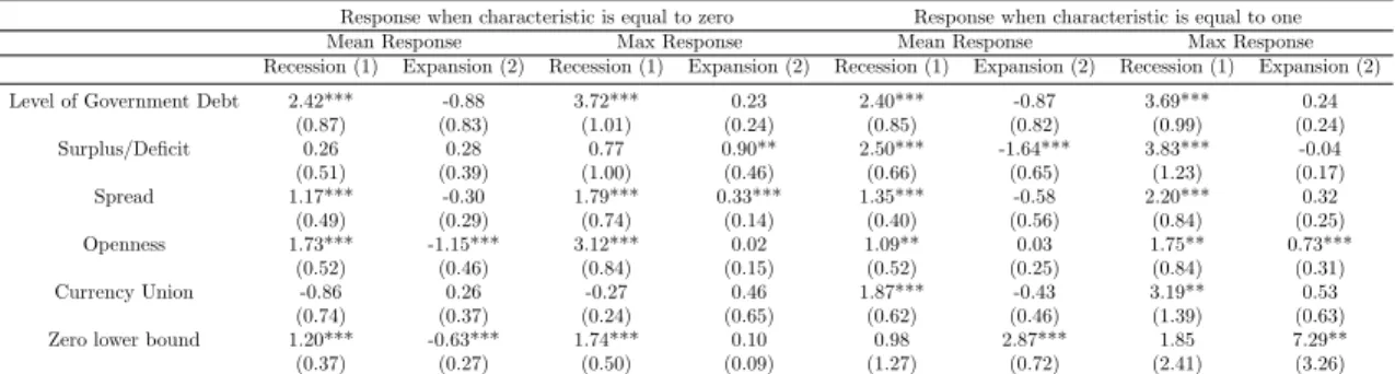
Table 1 reports the mean and the max response of output across countries over three year. We find that large government debt does not reduce the positive response of output to a government spending shock in a recession. In detail, when the debt to GDP ratio is low, a one percent increment in government purchases increases output about 2.42% over three years. Vice versa, if the level of debt is high, the mean response of output is 2.40%. Indeed, when the level of government debt is low, the max response of output is 3.72 whereas when the level of debt is high the max response is 3.70. The results do not show any adverse effect of public debt on the size of the fiscal multiplier.
Our estimates show that an increase in government spending during economic down-turns has a similar effect in countries with low and high public debt over three years. Conversely, when the economy is in expansion, an increase in government spending has no effect on GDP for both countries with high or low debt.
Besides the level of debt we investigate whether the presence of a high deficit or of an interest rate spread in the Eurozone countries affects the size of the spending multiplier. The empirical results show that an increase in public expenditure in high deficit countries during recession increases GDP approximately by 2.50%. In contrast, an increase in government spending in surplus/low deficit countries, has an output response of just 0.26% and is not statistically significant.19
19
The max response in the high deficit countries is 3.83%, whilst for surplus/low deficit countries is 0.77% and is not statistically significant.
We have similar results when we consider the spread, i. e. an indicator of relative financial risk. We find that the spending multiplier associated with an increase in govern-ment spending when the spread is above 150 basis point is larger than the one associated with an increase in government spending when the spread is under 150 basis point. In fact, the spending multiplier for the first case is 1.35 on average and reaches a maximum of 2.20 after three years. In contrast, the multiplier when the spread is under 150 basis point is 1.17 on average and reaches a maximum of 1.79 after three years. The Countries that have experienced a high sovereign risk are Spain (1991-1996), (2010-2014); Finland (1991-1995); Italy (1991-1996), (2011-2014); Portugal (1991-1996), (2010-2015); Belgium (2010) and Ireland (2010-2013). The results show that a stimulus to public spending, in downturns, is more effective to rise GDP in high risk countries than in “safe” countries.
The joint consideration of deficit and spread cases in Table 1 suggests that the stim-ulus effect of an increased government spending in recession is more effective in high deficit/spread countries than in low deficit/debt countries.20
The results of this section, joint with the negligible impact of public expenditure in-creases on the public debt/GDP ratio in recessions (section 4.2), cast doubts on the view that there was no alternative for high debt euro area countries but to go for fiscal consolid-ation in the midst of the 2011-2013 recession. The robustness of these results is confirmed by several tests. We have proved that an initial large public debt or an initial large public deficit or an initial wide spread do not reduce and actually enhance the response of private consumption, private investment and employment to a government spending shock.21
[Insert Table 1]
5.2 Multipliers in more and less open economies
Ilzetki et al. (2013) showed that the government spending multiplier is higher in closed economies than in open economies, which is consistent with the standard Macroeconomics literature. We find evidence that supports this prediction during recession. We show (Table 1) that for both open and closed economies22the mean and max response of output to a government spending shock is sizeable The size of government spending multiplier is higher for a closed economy, a one percent increase of government spending increases output of about 1.73%; in contrast for a open economy the mean response is as low as 1.09%.23
Corsetti et al. (2010, 2012) investigates whether the exchange rate regime determines the size of the fiscal multiplier. In the traditional Mundell-Fleming model, government spending is ineffective at stimulating domestic demand under flexible exchange rates be-cause a fiscal expansion “crowds out” net exports as a consequence of the exchange rate
20That means that a boost to aggregate demand (particularly for more risky countries ) will help to
speed up the recovery.
21Detailed results are available in the Appendix, Tables A1-A4. 22
The degree of openness is proxied by the ratio (export+import)/GDP. If for a country this ratio is higher than the average value for the sample countries, that country is “open”. Vice versa the country is “closed” if the above ratio is lower than the average value.
23
appreciation. In contrast, under fixed exchange rates, fiscal policy becomes effective be-cause the exchange rate appreciation is immediately offset through monetary expansion.
Since the European Monetary Union can be proxied by a fixed exchange rates regime as for the member countries, it is relevant to investigate whether the spending multiplier is higher in fixed exchange rate regime than in a flexible exchange rate regime. We show evidence that support this prediction. Under fixed exchange rates regime, a one percent increase in government spending during economic slack raises output by approximately 1.87%. In sharp contrast, under a fully flexible exchange rate regime (1985-1998) the response of output in recession is never significantly different from zero. The same results apply if one checks for the impact of the interaction between government spending increases and trade openness on private consumption, private investment and employment.24
5.3 Is the fiscal multiplier time varying?
Blanchard and Leigh (2013) emphasizes that during the “Great Recession” the size of fiscal multipliers has been underestimated. In order to investigate whether the Great Recession is different from previous recessions as regards the size of fiscal multipliers, we re-estimate the baseline formulation of model (1) for two sub-samples: pre-crisis (1985-2006) and crisis (2007-2105). In the (2007-2015) period the nominal interest rate in the Eurozone has been close to the zero lower bound. Panels 19-20 show the impulse responses of two macroeconomic variables (GDP and debt-GDP) to a one percent positive shock to government spending25. As usual, in each panel, there are two sub-panels showing the response (black, thick line for Recession and red, thick line for Expansion) in the two sub-periods (panel (a) before the Great Recession, panel (b) during the Great Recession). The thin dashed lines indicate the 80% confidence bands which are based on Newey and West (1987) standard errors that provide consistent estimates when there is autocorrelation in addition to possible heteroskedasticity of the error term in specification (1).26 Panel 19
shows that the spending multiplier is higher and statistically significant over the 3 years horizon in the period following the global financial crisis (Panel 19b, in recession). On the other hand, before the Great Recession, the spending multiplier reached its maximum after one year (2.24) and it became not statistical significant after the first year (Panel 19a, in recession). Conversely, when we consider the expansionary regime, the responses are quite analogous in both sub-samples The GDP response to an unexpected increase in government spending is negative but not statistically significant, before 2007 (Panel 19a), and it is near zero after 2007 (Panel 19b). Panel 20 presents the effect of an increase in government spending on the debt to GDP ratio. We control the effect of government spending shock on the debt to GDP ratio in order to account for the effect of a spending shock on the public budget. Panel 20b shows that an increase in government spending
24
Once again detailed results are available in the Internet Appendix, Tables A1-A4.
25We only show the results for the GDP and debt-GDP. The findings are similar when we consider
other macroeconomic variables, such as: private consumption, private investment, deficits; the results are available on request.
26The choice to increase the confidence interval is due to the fact that the observations in the sub-samples
leads to a decrease in the debt to GDP ratio over a 3 years’ horizon in the period following the Great Recession (2007-2015, in recession).
Before the outbreak of the crisis the effect of government spending on the debt to GDP ratio is strikingly different. An unexpected increase in government spending deteriorates the debt to GDP ratio over the 3 years’ horizon (Panel 20a, in recession). It is noteworthy that the debt multiplier follows a bell-shaped curve. The debt multiplier remains lower than one for about one year and a half; the second year it reaches its maximum (1.27) and then after the second year, it drops below one. Therefore, it is interesting to note, that it is true that an increase in government expenditure initially may deteriorate the debt to GDP ratio, however, the multiplier is almost always less than one (no multiplicative effect). Vice versa, in an expansionary regime, the impulse responses are quite similar in both sub-samples A government spending shock leads to an increase in the debt to GDP ratio both before 2007 and during the crisis (2007-2015).
[Insert Figure 6]
The results of this section confirm the exceptionality of the 2007-2015 crisis as com-pared to ordinary recessions in the period 1985-2006. The effectiveness of expansionary public spending shocks is magnified in the recent crisis years. Also, the effects of a public spending shock on the debt to GDP ratio proved to be different in the crisis years from what they used to be in more “normal” times. It may be observed that the Eurozone was actually close to the zero lower bound (ZLB) of nominal interest rates since 201127and that at the ZLB expansionary fiscal policies show enhanced effectiveness as the negative effect of interest rate increases in the face of expansionary (and potentially inflationary) fiscal policies are ruled out.28 To further investigate this issue we follow Miyamoto, Nguyen, Sergeyev (2017) and estimate the impact of an unforeseen positive shock to public ex-penditure respectively in the ZLB years (2011-2015) and in non-ZLB years (1985-2010), without distinguishing between recession and expansion. Panel 21a shows that a positive shock in the ZLB years is actually capable of triggering an output recovery. As monetary policy, in the period 1985-1998, was not in charge of a single central bank in EZ countries, we also controlled if our result is driven by the non-ECB years. After estimating our re-gressions for the sub-periods 1999-2010 and 2011-2015 we show that results do not change substantially (Panel 21b). The ZLB time span is short, and some North countries were already recovering in 2013-2014; hence our estimates should be considered with caution, and only used to explain why the fiscal multiplier in the Great Recession years are so much higher than in ordinary recessions.
27https://www.ecb.europa.eu/stats/policy and exchange rates/key ecb interest rates/html/
in-dex.en.html
28
Canzonieri et al. (2016), Christiano et al. (2011), Hall (2009), Erceg and Lind´e (2014) and Woodford (2011) derive in theoretical models fiscal multipliers on output which exceed one at the zero lower bound. In a different setting Eggertsson, Mehrotra, Robbins (2017) find that increases in government spending at the ZLB “can carry zero or negative multipliers [...], depending on the distribution of taxes across generations”. In an empirical investigation concerning Japan Miyamoto, Nguyen, Sergeyev (2017) estimate the effects of unexpected government spending increases both when the nominal interest rate is near the ZLB and outside of the ZLB period. They find an output multiplier equal to 1.5 on impact in the ZLB period, while it is as low as 0.7 outside of the ZLB period.
[Insert Figure 7]
6
Robustness Checks
In this section, we test the robustness of our findings in 2 ways: 1) we control for different variables that measure the state of the business cycle; 2) we re-estimate the fiscal multipli-ers distinguishing between countries with similar public public finance features, splitting our Eurozone sample into two groups (“South” countries vs “North” countries).
6.1 Is output responses depending on the variables that measure the state of business cycle?
In the baseline formulation of the empirical model, we use a moving average of the output growth rate to measure the state of the business cycle in each economy. The key advantage of using this variable is that the growth rate of output is a coincident indicator. Since the moving average is computed over 1.5 years and thus is cumulative, it should to some extent capture the output gap and thus the degree of slack in the economy. One may want to verify that using other measures of slack yields similar results. We employed alternative indicators of slack: (a) the de-trended log change in unemployment rate and (b) the de-trended log unemployment rate. In either case, we de-trend all series making use of the Hodrick-Prescott filter with smoothing parameter λ= 10,000. Irrespective of which measure we use, the response in a recession is larger than the response in expansion.29 We conclude that cyclical variation in the output responses is robust across different variables measuring the state of business cycle.
6.2 Southern Countries vs Northern Countries
In section 5.1 we found that an initial high level of public debt and deficit increases the size of fiscal multipliers in the Eurozone. As in the Eurozone there are two groups of countries differing as for their ratios of public deficit/debt to GDP and their fiscal space (South and North countries in short), in order to check the robustness of our findings we followed Bacchiocchi et al (2011) in re-estimating the baseline empirical model (1) by splitting the sample into two groups according to the level of public financial liabilities (as a share of GDP) during the sample period (1985-2015).30 The idea is to analyse whether the high/low deficit/debt countries are more or less affected by government spending shocks in the dif-ferent phases of business cycle. The results are shown in the Internet Appendix.31 This
29
The response sometimes are marginally statistically significant at 80 percent. Detailed results are available in the Internet Appendix (Figure A.1) for the GDP and debt-GDP.
30
Sample A (South Countries) comprises the GIIPS countries plus Belgium and France, which have either high debt or high deficit over the entire period. Sample B (North Countries) comprises Austria, Germany, Finland, Luxembourg and Netherlands. The results discussed below do not change if Greece, as an obvious outlier, is left out of Sample A.
31We only show the results for the GDP and debt-GDP (Figure A.2). The findings are analogous
even when we consider other macroeconomic variables, such as: private consumption, private investment, deficits; the results are available upon request.
robustness check strongly confirms the results obtained in section 5.1. To further invest-igate the question we also estimated the government multiplier by dropping one country at a time from the sample. Once again the results remain unchanged: the government multiplier turns out to be smaller when we drop one of the South countries and higher when we drop one of the North countries.32 We feel entitled to conclude that, contrary to conventional wisdom, an expansionary fiscal policy in a recession is more output-effective in South highly indebted countries than in North low-debt countries.
7
Conclusions
This paper brings together many strands of the empirical literature on the effects of fiscal policy (and of public expenditure in particular) on different macroeconomic aggregates in a unified analytical framework, featuring the local projection approach introduced by Jord´a (2005) that allows to construct impulse responses for any macroeconomic variable of interest, whilst being not constrained by the VAR’s restrictions. We focused on unforeseen government expenditure changes implemented in the Eurozone countries and estimated the effects of such policies on the key macroeconomic aggregates (GDP, private consump-tion, private investment), on public finance indicators (deficit, primary balance, debt to GDP ratio) and allowing the spending multipliers to vary smoothly according to the busi-ness cycle. This broad picture confirms for the Eurozone countries the existence of large differences in the size of public expenditure multipliers in recessions and in expansions, as found by Auerbach and Gorodnichenko (2013) for the broader OECD set of countries.
We find that an increase in public expenditure in the Eurozone has a high and positive multiplier effect on output, provided it is implemented in a recession, while this effect is negative or no-significant in expansions as predicted by Keynesian theory. Our analysis also shows that an expansionary fiscal policy in a recession has a strong “crowding in” effect on private consumption, whilst this crowding in effect on private investment is not statistically significant unless the policy implemented is surely countercyclical. Our es-timates also confirm that an expansionary fiscal policy in a recession does not impact on prices, real wages and unit labour cost, entailing that Eurozone countries could implement such a policy without deteriorating the price competitiveness of their exports. Counter-cyclical expansionary policies in a recession prove to be beneficial for the public budget on a five years horizon: both the deficit/GDP and the debt/GDP ratios would improve after the expansionary treatment. On the other hand, fiscal consolidations based on spending cuts, in a recession, prove to be non-expansionary and to raise both deficit and debt to GDP ratios over a not so short time horizon. The “expansionary austerity” view is not supported by our empirical results.
The paper further addresses a few highly debated issues concerning expenditure mul-tipliers in the Eurozone and shows: (i) in a recession fiscal mulmul-tipliers are higher in high debt countries than in low debt countries, implying that the absence of “fiscal space” does not cause the ineffectiveness of expansionary fiscal policies (the reverse in an expan-sion); (ii) under prevailing fixed exchange rates fiscal multipliers in a recession are greater
than under universal flexible exchange rates, implying that being in a monetary union actually enhances the effectiveness of expansionary fiscal policies (the reverse applies in expansions); (iii) increases in both government consumption and government investment have positive effects on output in a recession (negative in an expansion). However the effect of public investment is larger than that of public consumption in the long run (2 years after the shock); (iv) estimated fiscal multipliers were higher in the aftermath of the 2007-8 financial crisis than in previous recessions. This result is possibly associated with Eurozone experiencing the policy interest rate being near the zero lower bound during the recent prolonged recession/stagnation. All these results survive several robustness checks. Jeffrey Frankel said in 2014 conference, “what is the best fiscal policy, Austerity or Stimulus? The question is as foolish as the question ‘should a driver turn left or right?’ It depends where he is in the road. Sometimes left is the answer, sometimes right”. The empirical analysis carried out in this paper suggests that, under all respects, when the Euro countries are “in recession road” the correct answer is Stimulus, when the Euro countries are in “expansion road” the correct answer is Austerity. From our findings one may say that the aftermath of the sovereign debt crisis was not the right time to implement a fiscal consolidation in many Eurozone countries.
References
Abiad, A. d, Furceri, D., Topalova, P. (2015). “The Macroeconomic Effects of Public Investment; Evidence from Advanced Economies”. IMF Working Papers 15/95, Interna-tional Monetary Fund.Alesina, A., Perotti, R. (1995). “Fiscal expansions and adjustments in OECD countries”. Economic Policy, 21 (10): 207-248.
Alesina, A., Favero,C., Giavazzi, F. (2015). “The output effect of fiscal consolidations”. Journal of International Economics, 96 S(1): 19–42.
Auerbach, A. J., Gorodnichenko, Y. (2012a). “Measuring the Output Responses to Fiscal Policy”. American Economic Journal : Economic Policy, 4 (2): 1-27.
Auerbach, A. J., Gorodnichenko, Y. (2012b). “Output Spillovers from Fiscal Policy”. NBER Working Paper 18578.
Auerbach, A. J., Gorodnichenko, Y. (2013). “Fiscal Multipliers in Recession and Expansion”. In Fiscal Policy after the Financial Crisis, edited by Alberto Alesina and Francesco Giavazzi. Chicago: University of Chicago Press.
Auerbach, A. J., Gorodnichenko, Y. (2014). “Fiscal Multipliers in Japan”. NBER Working Papers 19911.
Baxter, M., King, R. G. (1993), “Fiscal Policy in General Equilibrium”. American Economic Review,83 (3): 315-334.
Bachmann, R., Sims, E. (2012). “Confidence and the transmission of government spending shocks”. Journal of Monetary Economics, 59(3): 235-49.
Barro, R. J., Redlick, C. J. (2011). “Macroeconomic effects from government purchases and taxes”. Quarterly Journal of Economics, 126 (1): 51-102.
Baum A., Poplawski-Ribeiro, M., Weber, A. (2012). “Fiscal Multipliers and the State of the Economy”. IMF Working Papers 12/286, International Monetary Fund.
effects of changes in government spending and taxes on output”. Quarterly Journal of Economics, 117(4): 1329-1368.
Blanchard, O. J., Giavazzi, F. (2004), “Improving the SGP Through a Proper Ac-counting of Public Investment”. CEPR Discussion Papers 4220.
Blanchard, O., Erceg, C., Linde, J., (2015). “Jump starting the euro area recovery: would a rise in core fiscal spending help the periphery?”. NBER Working Paper 21426.
Blanchard, O.J., Leigh,D. (2013). “Growth Forecast Errors and Fiscal Multipliers”. American Economic Review, 103(3): 117-120.
Blanchard,O. J., Dell’Ariccia, G., Mauro, P. (2013). “Rethinking Macro Policy II; Getting Granular”. IMF Staff Discussion Notes 13/003, International Monetary Fund.
Callegari, G., Melina, G., Batini,N. (2012). “Successful Austerity in the United States, Europe and Japan”. IMF Working Papers 12/190, International Monetary Fund.
Canova, F., Pappa, E. (2011). “Fiscal policy, pricing frictions and monetary accom-modation”. Economic Policy, 26(68): 555-598.
Canzoneri,M., Collard,F., Dellas, H., Diba, B. (2016). “Fiscal Multipliers in Reces-sions”. Economic Journal, 126(590): 75-108.
Christiano, L., Eichenbaum, M., Rebelo, S. (2011). “When is the government spending multiplier large?”. Journal of Political Economy, 119(1): 78-121.
Cimadomo, J., B´enassy-Qu´er´e, A. (2012). “Changing patterns of fiscal policy mul-tipliers in Germany, the UK and the US”. Journal of Macroeconomics, Elsevier, 34(3): 845-873.
Cloyne, J. (2013). “Discretionary Tax Changes and the Macroeconomy: New Narrative Evidence from the United Kingdom”. , American Economic Review, 103(4): 1507-28.
Coenen, G., C. J. Erceg, C. Freedman, D. Furceri, M. Kumhof, R. Lalonde, D. Laxton, et al. (2012). “Effects of Fiscal Stimulus in Structural Models”. American Economic Journal: Macroeconomics, 4 (1): 22-68.
Cogan, J., Cwik, T., Taylor, J., Wieland, V. (2010). “New Keynesian versus old Keynesian government spending multipliers”. Journal of Economic Dynamics and Con-trol, 34(3): 281-95.
Corsetti, G., Meier, A., M¨uller,G. J. (2012). “What determines government spending multipliers?”. Economic Policy, CEPR;CES;MSH, 27(72): 521-565, October.
Corsetti, G., Kuester,K., Meier, A., M¨uller, G.J. (2010). “Debt consolidation and fiscal stabilization of deep recessions”. American Economic Review, Papers and Proceedings, 100 (2): 41-45.
Curdia, V., Woodford, M. (2010). “Credit spreads and monetary policy”. Journal of Money, Credit and Banking, 42(S1): 3-35.
De Grauwe, P., Yuemei Ji (2012). “Mispricing of sovereign risk and macroeconomic stability in the eurozone”. Journal of Common Market Studies, 50 (6),pp. 866-880.
De Long, J. B., Summers, L. H. (2012). “Fiscal policy in a depressed economy”. Brookings Papers on Economic Activity, 1: 233-274.
Drautzburg, T., Uhlig, H. (2011), “Fiscal Stimulus and Distortionary Taxation”. NBER Working Paper 17111.
Eggertsson, G. B. (2011), “What Fiscal Policy is Effective at Zero Interest Rates?”. NBER Macroconomics Annual, 25: 59-112).