Advances in Bayesian Inference for Binary and Categorical Data

(1)

PhD SCHOOL

PhD program in Statistics

Cycle: XXXII

Disciplinary Field: SECS-S/01

Advances in Bayesian Inference for Binary and

Categorical Data

Advisor: Prof. Daniele Durante

Co-Advisor: Prof. Igor Prünster

PhD Thesis by

Augusto Fasano

ID number: 3029881

(2)

Bayesian binary probit regression and its extensions to time-dependent observations and multi-class responses are popular tools in binary and categorical data regression due to their high interpretability and non-restrictive assumptions. Although the theory is well established in the frequentist literature, such models still face a florid research in the Bayesian framework. This is mostly due to the fact that state-of-the-art methods for Bayesian inference in such settings are either computationally impractical or inaccurate in high dimensions and in many cases a closed-form expression for the posterior distri-bution of the model parameters is, apparently, lacking. The development of improved computational methods and theoretical results to perform inference with this vast class of models is then of utmost importance.

In order to overcome the above-mentioned computational issues, we develop a novel variational approximation for the posterior of the coefficients in high-dimensional probit regression with binary responses and Gaussian priors, resulting in a unified skew-normal (SUN) approximating distribution that converges to the exact posterior as the number of predictors p increases. Moreover, we show that closed-form expressions are actually available for posterior distributions arising from models that account for correlated bi-nary time-series and multi-class responses. In the former case, we prove that the filtering, predictive and smoothing distributions in dynamic probit models with Gaussian state vari-ables are, in fact, available and belong to a class of SUN distributions whose parameters can be updated recursively in time via analytical expressions, allowing to develop an i.i.d. sampler together with an optimal sequential Monte Carlo procedure. As for the latter case, i.e. multi-class probit models, we show that many different formulations developed in the literature in separate ways admit a unified view and a closed-form SUN posterior distribution under a SUN prior distribution (thus including the Gaussian case). This allows to implement computational methods which outperform state-of-the-art routines in high-dimensional settings by leveraging SUN properties and the variational methods introduced for the binary probit.

Finally, motivated also by the possible linkage of some of the above-mentioned models to the Bayesian nonparametrics literature, a novel species-sampling model for partially-exchangeable observations is introduced, with the double goal of both predicting the class (or species) of the future observations and testing for homogeneity among the different available populations. Such model arises from a combination of Pitman-Yor processes and leverages on the appealing features of both hierarchical and nested structures developed in the Bayesian nonparametrics literature. Posterior inference is feasible thanks to the implementation of a marginal Gibbs sampler, whose pseudo-code is given in full detail.

(3)

Acknowledgements

The completion of present thesis would have certainly not been possible without the great mentorship of my two thesis advisors, Prof. Daniele Durante and Prof. Igor Pr¨unster. I would then like to express my most sincere gratitude to Daniele for constantly supporting my Ph.D. research with contagious enthusiasm, which allowed me to truly enjoy doing research, in addition to continuously motivating me to do my best. I knew I could count on him and on his countless ideas when I needed a helping hand to figure out in which direction I should move for my research. On the other hand, I would certainly not be here if it was not for Igor, to whom I am deeply grateful for motivating me to pursue a Ph.D. and for guiding me across research since I was an Allievo at Collegio Carlo Alberto in Turin: his patience, his immense knowledge and his guidance across years were fundamental to get to the end of this Ph.D. thesis, which I hope will be a new beginning. I am certain I could have not hoped to have better Ph.D. supervisors.

I should also thank Giacomo Zanella for his great availability and for all the things he made me learn each time I passed by his office. Moreover, I am also extremely grateful to my Ph.D. colleague and friend Giovanni Rebaudo: thanks to him I could have a lot of fun in doing research, and I hope we will enjoy research together also in the future. Last but not least, I could have hardly pursued this Ph.D. without the support of my parents, to whom it goes my sincere gratitude.

(4)

Chapter 1 Introduction

Regression models for dichotomous and categorical data are facing a considerable interest, due to their wide range of possible applications, spanning across many fields of research (Agresti, 2013,2018). Such models are suited to study how the probability mass function of a categorical response variable y—that is, a variable whose measurement scale consists in a set of categories—changes with a set of observed predictors x ∈ Rp_{. Such categorical}

outcomes are widespread in health sciencies, social and political sciences, econometrics, machine learning and statistics in general. Just to mention a few examples of practical relevance (seeAgresti (2018) for additional applications), y could represent the severity of an injury (“none”, “mild”, “moderate”, “severe”), or the type of a tumor mass, including both the dichotomous case “benignant” vs “malignant” or more granular outcomes as “benignant”, “malignant type 1”, “malignant type 2”. In social sciences applications, where the interest is in measuring attitudes and opinions, categorical responses regression models are used to study political orientation (“Democrat” vs “Republican” or multi-class) as well as preferences among different alternatives that customers face, in the so-called discrete-choice scenarios (see Greene (2003) for a detailed overview). The range of other possible applications is huge, as they can be used in standard classification tasks, like email spam detection (“spam” vs “legitimate mail”), handwritten digit classification (Rasmussen and Williams, 2006), or to model the occurrence of a certain event (yes, no), like the presence of a certain disease or the rise of a stock price in a trading day.

Although the frequentist theory is now well-established (Agresti, 2013), Bayesian in-ference for binary and categorical data regression models is still an open area of research, both from a methodological and computational standpoint. Many of these models, includ-ing the ones considered in the present thesis, admit an interpretation in terms of latent (unobserved) continuous data, which can be used to get further insights on theoretical properties of the model at hand and to perform Bayesian computations (Albert and Chib, 1993, 2001;Consonni and Marin, 2007;Andrieu and Doucet, 2002;McCulloch and Rossi, 1994; Imai and Van Dyk, 2005; Girolami and Rogers, 2006; Girolami and Zhong, 2007).

(8)

In particular, the present thesis focuses on computational and methodological advances in Bayesian inference for the binary probit model, together with more sophisticated con-structions to account for correlated binary time series and categorical data. Considering for the moment the probit model for binary outcomes for ease of exposition, each obser-vation yi is a Bernoulli random variable with mean parameter pr(yi = 1 | β) = Φ(x|iβ),

being β ∈ Rp _{the parameter vector of the effects of each covariate on the output. Such a}

model admits a dual interpretation in terms of partially observed latent Gaussian random variables: it can indeed be rewritten as yi = 1[zi > 0], with zi ∼ N(x|iβ, 1) and 1[·] the

indicator function. See Chapter 2 for further details.

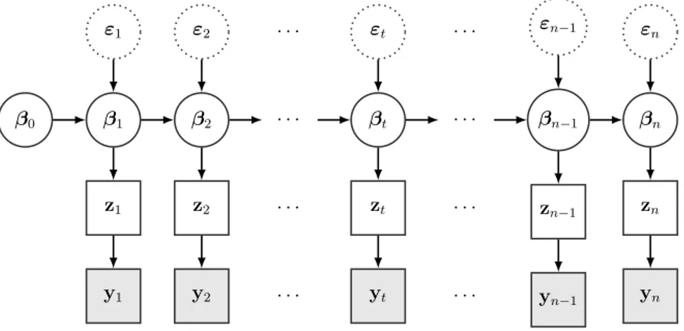
Such latent variables can be used as auxiliary variables or can have an interpretable meaning: in the voting example reported above, they can for instance represent a contin-uous measure of voter i’s preference towards one of the two parties, ending up in her/him voting that party if such continuous-valued measure falls above zero. Similar concepts of underlying continuous latent variables driving the observations are present also when one considers extensions of the probit model to account for dependent binary time series or multi-class responses. Such models are studied in detail in Chapters 3 and 4 of the present thesis, respectively: the corresponding latent continuous-valued process is a multivariate dynamic linear model (Petris et al., 2009) in the former case and a set of unobserved utilities, one for each possible choice, in the latter case (Greene, 2003).

As apparent from the previous arguments, all these models arise from a hierarchical construction. It comes then with no surprise that Bayesian hierarchical models have been widely used in such contexts, as they represent a natural tool to interpret the model construction and perform posterior inference. However, the apparent lack of a conjugate prior distribution for all these classes of probit models motivated a rich literature for computational methods in order to perform Bayesian inference in these settings, due to their central role in binary and categorical Bayesian data analysis. See Chapters 2, 3 and 4 and references therein for more detailed literature reviews. Most of the available methods rely on Markov-Chain Monte Carlo (mcmc) methods to sample from the pos-terior distribution, exploiting the above-mentioned hierarchical constructions to develop a Gibbs sampler (Albert and Chib, 1993;Holmes and Held, 2006; Pakman and Paninski, 2014; Imai and Van Dyk, 2005). Approximate methods have also been developed for the binary and categorical probit models (Consonni and Marin, 2007; Chopin and Ridgway, 2017; Girolami and Rogers, 2006_{), while state-of-the-art sequential Monte-Carlo (smc)}

routines (Andrieu and Doucet, 2002) provide the standard tool for online inference in the univariate binary time-series setting. However, the available mcmc methods are imprac-tical in large p scenarios, and approximate methods either suffer the same computational problems (Chopin and Ridgway, 2017) or are inaccurate (Consonni and Marin, 2007).

A first solution to these methodological and computational bottlenecks was recently given by Durante (2019), who showed a conjugacy result for the probit model for binary

(9)

data with Gaussian priors on the coefficients. This finding, in addition to provide a deeper theoretical understanding of the posterior distribution of the model parameters, allows to implement computational strategies for posterior inference that outperform stat-of-the-art routines in the large p small n scenario, though leaving the computation or approximation of the posterior an open research question when p is large and n is moderate-to-large. Such a problem is tackled in Chapter 2, where a novel variational approximation of the poste-rior distribution of the binary probit model under Gaussian pposte-riors is developed. Durante (2019) showed that, within such a framework, the posterior distribution for the p probit coefficients has a unified skew-normal (SUN) kernel (Arellano-Valle and Azzalini, 2006;

Azzalini and Capitanio, 2014), which can be expressed via a convolution of a p-variate normal and an n-variate truncated normal with full covariance matrix. As the latter part is the main reason for the computational inefficiency as n increases, we propose a varia-tional approximation for the SUN posterior distribution, which factorizes the multivariate truncated normal density via a product of univariate truncated normal densities. Such a result can be formally interpreted as a partially factorized mean-field variational Bayes strategy (Bishop, 2006; Blei et al., 2017) which provides a tighter approximation to the posterior distribution for the probit coefficients, compared to state-of-the-art solutions in Bayesian variational inference (Consonni and Marin, 2007), while crucially preserving skewness. Such a method is proven to be asymptotically exact as the number of covari-ates p diverges: in such a case, the Kullback-Leibler divergence (Kullback and Leibler, 1951) between the variational approximation and the exact posterior goes to zero with probability one.

Motivated by the above-mentioned methodological and computational advances, other interesting research questions involve the extension of such results to the frameworks of time-dependent binary observations and multi-class probit models mentioned above. We address these questions in Chapters 3 and 4, respectively. Considering the binary time series case, studied in Chapter 3, it admits an interpretation in terms of a partially-observed dynamic linear model (Petris et al., 2009; Durbin and Koopman, 2012). In this framework, when one considers usual Gaussian-Gaussian dynamic linear models, all the distributions of interest are available in closed-form, thanks to the well-known Kalman filter (Kalman, 1960). However, when we move to the non-Gaussian binary case, such a routine is lacking in the literature, leaving it an open research question, which we successfully tackle. Indeed, even though smc methods are efficient in performing online inference in binary time-series analysis, they are still sub-optimal with respect to closed-form expressions or exact sampling methods. Moreover, they suffer from the well-known problem of particle degeneracy (Durbin and Koopman, 2012) when one moves from online, i.e. filtering and predictive, to batch, i.e. smoothing, inference, leaving the joint and marginal smoothing an open research question. In Chapter 3, we prove that the filtering, predictive and smoothing distributions of dynamic probit models with Gaussian

(10)

state variables belong to the class of unified skew-normals (SUN) and that a closed-form expression for the observation predictive probability is available. Leveraging on SUN properties (Arellano-Valle and Azzalini, 2006; Azzalini and Capitanio, 2014; Durante, 2019), we propose methods to draw independent and identically distributed (i.i.d.) samples from the joint smoothing distribution, which can easily be adapted to obtain i.i.d. samples from filtering and predictive distributions, thereby improving state-of-the-art approximate or sequential Monte Carlo inference in small-to-moderate dimensional dynamic models. A scalable and optimal (in the sense ofDoucet et al. (2000)) particle filter which exploits sun properties is also developed in order to deal with online inference in large dimensional dynamic models.

Extensions of the binary probit model do not stop to binary time series, but include a large class of models for multi-class outputs. Many different constructions, with associated mcmc procedures, have been proposed in the literature (Hausman and Wise, 1978;Tutz,

1991; Stern, 1992; McCulloch and Rossi, 1994; McCulloch et al., 2000; Albert and Chib, 2001; Imai and Van Dyk, 2005). However, a unified view on them is lacking at the moment, as well as a closed-form expression for the corresponding posterior distributions. The goal of Chapter 4 is indeed to provide such a unified view, together with theoretical and computational advances, on models for categorical data that can be formulated as extensions of the binary probit model, generally referred to as Multinomial Probit (MNP) models. We focus in particular on the original formulation by Hausman and Wise (1978), on an alternative model with class-specific parameters (Stern, 1992) and on a sequential construction arising from initial formulations byTutz (1991) andAlbert and Chib (2001). We show that all the three models, originally developed in a separate way for different kinds of data, lead to a SUN posterior distribution of the parameters under a SUN (and hence also Gaussian) prior distribution, developing an efficient sampling procedure which outperforms state-of-the-art methods in the large p moderate n scenario. Such results are then used as a starting point to develop variational inference techniques extending the routine introduced in Chapter 2, allowing to get posterior estimates when both p and n are large, with particular focus on the case p > n.

All the models discussed so far deal with probabilistic classification, so that predictions about future observations will be given in the form of class probabilities and not only as point class predictions: class guesses can then be obtained as solutions of a decision problem, after the specification of a loss-function. A research area strictly related to this probabilistic classification framework is given by the Bayesian nonparametrics approach to species sampling problems, introduced in Lijoi et al. (2007), where the main interest is in prediction of additional observations, conditionally on the available data. In particular, key quantities to predict are the number of new species in an additional sample, which can be seen as a measure of species diversity, or the rate of decay of the probability of discovering new species. Frequentist analogs originated in connection with ecological

(11)

problems (Good, 1953; Good and Toulmin, 1956). Since then, however, they have been applied in various other fields, so that the term ‘species’ has actually gained a metaphoric meaning and can indicate different possible types, genes, agents or categories, depending on the context. In particular, these models are facing an increasing interest in the Bayesian nonparametrics community, with a wide range of applications spreading across genetics (Lijoi et al., 2007; Favaro et al., 2009, 2012), economics (Lijoi et al., 2016) and machine learning (Teh, 2006). See also De Blasi et al. (2015) for an extensive overview. In this framework, the most used model is arguably the Pitman Yor Process (PYP) (Pitman and Yor, 1997), being it preferred to the popular Dirichlet Process (DP) (Ferguson, 1973) mainly due to the fact that the probability that a new observation forms a new cluster, conditionally on the available sample, depends on the number of already created clusters, providing greater flexibility than the DP, where such probability depends only on the overall sample size. This is also reflected in different asymptotic distributions for the number of observed clusters as the population size diverges, with the PYP showing a power-law behaviour, which is common in many empirical studies (Mitzenmacher, 2004;

Goldwater et al., 2006), contrary to the logarithmic growth observed for the DP, which appears too restrictive.

When moving to the partially exchangeable framework, where multiple samples are collected across different, but related, studies, Bayesian hierarchical models have proved to be an effective tool, since they naturally allow to borrow information across groups (Teh et al., 2006;Teh, 2006; Teh and Jordan, 2010; Camerlenghi et al., 2019b). Such hi-erarchical constructions, although quite flexible, do not allow to have ties of distributions of various groups, so that these will have different, but related, distributions. A popular practice to specify a model that allows for ties among distributions of different groups is to exploit nested structures (Rodr´ıguez et al., 2008;Camerlenghi et al., 2019a). However, these models either suffer from a degeneracy issue that does not allow ties in the obser-vations across different groups without degenerating to the exchangeable case (Rodr´ıguez et al., 2008), or are computationally infeasible for more than two groups (Camerlenghi et al., 2019a). For these reasons, none of them is suitable to perform population homo-geneity testing in species sampling models with more than two groups.

Motivated by this methodological and computational lack, in Chapter 5 we introduce a novel species-sampling model for the multiple-sample setting, allowing predictive inference of future observations as well as clustering of the different population distributions, so to perform population homogeneity testing. Such model arises by combining PYPs in a way to exploit the advantages of both the hierarchical and nested constructions developed in the Bayesian nonparametrics literature (Teh et al., 2006; Teh, 2006; Rodr´ıguez et al., 2008; Teh and Jordan, 2010;Camerlenghi et al., 2019a,b).

In order to do so, we extend the Hierarchical Pitman-Yor process (HPYP) (Teh, 2006) by adding a latent structure on the population distributions, so that we allow ties across

(12)

them and we can perform both the above-mentioned tasks at the same time. We then show that the distribution of the induced random partition admits a closed-form expression, which allows to gain a deeper insight on the theoretical properties of the model. Posterior inference is feasible thanks to an mcmc routine which allows to evaluate the functionals of interest and to perform homogeneity testing for different populations with multiple groups.

(13)

Chapter 2 Variational Bayes for

High-Dimensional Probit Models

2.1 Introduction

The absence of tractable posterior distributions in several Bayesian models, and the recent abundance of high-dimensional datasets have motivated a growing interest in strategies for scalable learning of approximate posteriors, beyond classical sampling-based Markov chain Monte Carlo (mcmc) methods (e.g., Green et al., 2015). Deterministic approxi-mations, such as variational Bayes (vb) (Blei et al., 2017) and expectation-propagation (ep) (Minka, 2001), provide powerful approaches to improve computational efficiency in posterior inference. However, in high-dimensional models these methods still face open problems in terms of scalability and quality of the posterior approximation. Notably, such issues also arise in basic predictor-dependent models for binary responses (Agresti, 2013), which are routinely used and provide a building block in several hierarchical models (e.g.,

Chipman et al., 2010;Rodriguez and Dunson, 2011). Recalling a recent review byChopin and Ridgway (2017), the problem of posterior computation in binary regression is partic-ularly challenging when the number of predictors p becomes large. Indeed, while standard sampling-based algorithms and deterministic approximations can easily deal with small p problems, these strategies are impractical when p is large; e.g., p > 1000.

Classical specifications of Bayesian regression models for binary data assume that the dichotomous responses yi ∈ {0; 1}, i = 1, . . . , n, are conditionally independent

re-alizations from a Bernoulli variable Bern[g(x|_iβ)], given a fixed p-dimensional vector of predictors xi = (xi1, . . . , xip)| ∈ Rp, i = 1, . . . , n, and the associated coefficients

β = (β1, . . . , βp)| ∈ Rp. The mapping g(·) : R → (0, 1) is commonly specified to be

either the logit or probit link, thus obtaining pr(yi = 1 | β) = [1 + exp(−x|iβ)] −1 _in

the first case, and pr(yi = 1 | β) = Φ(x|iβ) in the second, where Φ(·) is the cumulative

(14)

models, it is common practice to specify Gaussian priors for the coefficients β, and then update such priors with the likelihood of the observed data y = (y1, . . . , yn)| to obtain

the posterior p(β | y), which is used for point estimation, uncertainty quantification and prediction. However, the apparent absence of conjugacy in this Bayesian updating moti-vates the use of computational strategies relying either on Monte Carlo integration or on deterministic approximations (Chopin and Ridgway, 2017).

A popular class of mcmc methods that has been widely used in applications of Bayesian regression for binary data leverages augmented data representations which allow the implementation of tractable Gibbs samplers relying on conjugate full-conditional dis-tributions. In Bayesian probit regression this strategy exploits the possibility of expressing the binary data yi ∈ {0; 1}, i = 1, . . . , n, as dichotomized versions of an underlying

re-gression model for Gaussian responses zi ∈ R, i = 1, . . . , n, thereby restoring conjugacy

between the Gaussian prior for the coefficients β and the augmented data, which are in turn sampled from truncated normal full-conditionals (Albert and Chib, 1993). More re-cently, Polson et al. (2013) proposed a related strategy for logit regression which is based on a representation of the logistic likelihood as a scale mixture of Gaussians with respect to P´olya-gamma augmented variables zi ∈ R+, i = 1, . . . , n. Despite their simplicity,

these methods face well-known computational and mixing issues in high-dimensional set-tings, especially with imbalanced datasets (Johndrow et al., 2019). We refer to Chopin and Ridgway (2017) for a discussion of related data-augmentation strategies (Holmes and Held, 2006; Fr¨uhwirth-Schnatter and Fr¨uhwirth, 2007) and alternative sampling meth-ods, such as adaptive Metropolis–Hastings (Roberts and Rosenthal, 2001; Haario et al., 2001) and Hamiltonian Monte Carlo (Hoffman and Gelman, 2014), among others. While these strategies address some disadvantages of data-augmentation Gibbs samplers, they are still computationally impractical in large p applications (Chopin and Ridgway, 2017;

Nishimura and Suchard, 2018; Durante, 2019).

A possible solution to scale-up computations is to consider deterministic approxima-tions of the posterior distribution. In binary regression contexts, two strategies that have gained growing popularity are mean-field (mf) vb with global and local variables (Jaakkola and Jordan, 2000;Consonni and Marin, 2007;Durante and Rigon, 2019_{), and ep}

(Chopin and Ridgway, 2017). The first class of methods approximates the joint posterior density p(β, z | y) for the global parameters β = (β1, . . . , βp)| and the local augmented

data z = (z1, . . . , zn)| with an optimal factorized density q_mf∗ (β)

Qn i=1q

∗

mf(zi) which is the

closest in Kullback–Leibler divergence (Kullback and Leibler, 1951) to p(β, z | y), among all the approximating densities in the mean-field family Q_mf = {q_mf(β, z) : q_mf(β, z) = q_mf(β)q_mf(z)}. Optimization typically proceeds via coordinate ascent variational inference methods (cavi) which can scale easily to large p settings. However, mf-vb is known to underestimate posterior uncertainty and often leads to Gaussian approximations which affect the quality of inference if the actual posterior is non-Gaussian (Kuss and

(15)

Ras-mussen, 2005). As we will show in Sections 2.2 and 2.3, this issue can have dramatic implications in the setting considered in this chapter. Also ep provides Gaussian ap-proximations (Chopin and Ridgway, 2017_{), but typically improves the quality of vb via}

a moment matching of approximate marginals that have the same factorized form of the actual posterior. These gains come, however, with a computational cost which makes ep not practical for high-dimensional settings with, e.g., p > 1000. Indeed, recalling a concluding remark by Chopin and Ridgway (2017), the lack of scalability to large p is common to most state-of-the-art methods for Bayesian computation in binary regression models. An exception is provided by the recent contribution of Durante (2019), which proves that in Bayesian probit regression with Gaussian priors the posterior actually be-longs to the class of unified skew-normal (SUN) distributions (Arellano-Valle and Azzalini, 2006). These variables have several closure properties which facilitate posterior inference in large p settings. However, the calculation of relevant functionals for inference and pre-diction requires the evaluation of cumulative distribution functions of n-variate Gaussians or sampling from n-variate truncated normals, thus making these results impractical in a variety of applications with sample size n greater than a few hundreds (Durante, 2019).

In this chapter we address most of the aforementioned issues by proposing a new partially factorized mean-field approximation (pfm) for Bayesian probit regression which avoids assuming independence between the global variables β and the augmented data z. Unlike ep (Chopin and Ridgway, 2017_{), the proposed pfm-vb scales easily to p 1000}

settings, and, unlike for the computational strategies proposed in Durante (2019), it only requires evaluation of distribution functions of univariate Gaussians. Moreover, despite having a computational cost comparable to standard mf-vb for probit models (Consonni and Marin, 2007_{), the proposed pfm-vb leads to a substantially improved approximation}

of the posterior in large p settings, which reduces bias in locations and variances, and crucially incorporates skewness. Optimization proceeds via a simple cavi algorithm and provides a tractable SUN approximating density. The methodology is discussed in Sec-tion 2.2, where we also provide theoretical results showing that the pfm-vb approximaSec-tion converges to the exact posterior as p → ∞, and that the number of iterations required by the cavi to find the optimum converges to 1 as p → ∞. Insightful negative results on the accuracy of standard mf-vb approximations, that suggest caution against maximum a posteriori inferences in high-dimensional contexts, are also provided. The proposed methods are evaluated on an Alzheimer’s application with p = 9036 in Section 2.3. Con-cluding remarks and proofs can be found in Section 2.4 and in Appendix 2.A, respectively. Finally, Appendix 2.B discusses the computational complexity of the proposed inference and optimization strategies which can crucially be performed at an O(pn·min{p, n}) cost. Codes and tutorials to implement the proposed methods and reproduce the analyses are

(16)

2.2 Variational Bayesian Inference for Probit Models

Recalling Section 2.1, we focus on posterior inference for the classical Bayesian probit regression model defined as

(yi | β) ind

∼ Bern[Φ(x|_iβ)], i = 1, . . . , n, β ∼ Np(0, νp2Ip).

(2.1)

In (2.1), each yi is a binary variable whose success probability depends on a p-dimensional

vector of observed predictors xi = (xi1, . . . , xip)| under a probit mapping. The

coeffi-cients β = (β1, . . . , βp)|regulate the effect of each predictor and are assigned independent

Gaussian priors βj ∼ N(0, νp2), for every j = 1, . . . , p. Although our contribution can

be naturally generalized to a generic multivariate Gaussian prior for β, we consider here the simpler setting with β ∼ Np(0, νp2Ip) to ease notation, and allow the prior variance

ν2

p to possibly change with p. This choice incorporates not only routine

implementa-tions of Bayesian probit models relying on constant prior variances ν2

p = ν2 for the

co-efficients (e.g., Chopin and Ridgway, 2017), but also more structured formulations for high-dimensional problems which define ν2

p = ν2/p to control the prior variance of the

en-tire linear predictor and induce increasing shrinkage (e.g., Simpson et al., 2017; Fuglstad et al., 2018). The prior variance coefficient ν2

p is allowed to vary with p, in order to

ac-commodate for most common routine implementations of Bayesian probit models, where either ν2

p = ν2 and hence the coefficients are considered a priori independent with

con-stant variance (e.g., Chopin and Ridgway, 2017) or ν2

p = ν2/p so that the variance of

the linear predictor is kept constant (e.g., Fuglstad et al., 2018). Details on the technical assumptions for the asymptotic behavior of ν2

p are stated in Assumption A2.

Model (2.1) also has a simple constructive representation based on Gaussian aug-mented data, which has been broadly used in the development of mcmc (Albert and Chib, 1993_{) and vb (}Consonni and Marin, 2007) methods. More specifically, (2.1) can be obtained by marginalizing out the augmented data z = (z1, . . . , zn)| in the model

yi =1(zi > 0), (zi | β) ind ∼ N(x|_iβ, 1), i = 1, . . . , n, β ∼ Np(0, νp2Ip). (2.2)

Recalling Albert and Chib (1993), the above construction leads to closed-form full-conditionals for β and z, thus allowing the implementation of a Gibbs sampler where p(β | z, y) = p(β | z) is a Gaussian density, and each p(zi | β, y) = p(zi | β, yi)

is the density of a truncated normal, for i = 1, . . . , n. We refer to Albert and Chib (1993) for more details regarding such a strategy. Our focus here is on large p settings where classical mcmc is often impractical, thus motivating more scalable methods relying

(17)

on approximate posteriors. In Section 2.2.1, we discuss standard mf-vb strategies for Bayesian probit models (Consonni and Marin, 2007) which rely on representation (2.2), and prove that in large p settings these approaches lead to poor approximations of the exact posterior that underestimate not only the variance but also the location, thus leading to unreliable inference and prediction. In Section 2.2.2, we address these issues via a new partially factorized variational approximation that has substantially improved practical and theoretical performance in large p settings, especially when p n.

2.2.1 Mean-field variational Bayes

Recalling Blei et al. (2017_{), mean-field vb with global and local variables aims at}

pro-viding a tractable approximation for the joint posterior density p(β, z | y) of the global parameters β = (β1, . . . , βp)| and the local variables z = (z1, . . . , zn)|, within the mf

class of factorized densities Q_mf = {q_mf(β, z) : q_mf(β, z) = q_mf(β)q_mf_{(z)}. The optimal vb} solution q_mf∗ (β)q_mf∗ (z) within this family is the one that minimizes the Kullback–Leibler (kl) divergence (Kullback and Leibler, 1951) defined as

kl[qmf(β, z) || p(β, z | y)] = Eqmf(β,z)[log qmf(β, z)] − Eqmf(β,z)[log p(β, z | y)], (2.3) with q_mf(β, z) ∈ Q_mf. Alternatively, it is possible to obtain q_mf∗ (β)q_mf∗ (z) by maximizing

elbo[qmf(β, z)] = Eqmf(β,z)[log p(β, z, y)] − Eqmf(β,z)[log q(β, z)], (2.4) with q_mf(β, z) ∈ Q_mf_{, since the elbo coincides with the negative kl up to an additive} constant. Recall also that the kl divergence is always non-negative and refer toArmagan and Zaretzki (2011_{) for the expression of elbo[q}_mf(β, z)] under (2.2). The maximization of (2.4) is typically easier than the minimization of (2.3), and can be performed via a simple coordinate ascent variational inference algorithm (cavi) (e.g., Blei et al., 2017) cycling among the two steps below

q(t)_mf_{(β) ∝ exp{E}_q(t−1) mf (z) log[p(β | z, y)]}, q_mf(t)_{(z) ∝ exp{E}_q(t) mf(β) log[p(z | β, y)]}, (2.5)

where q_mf(t)(β) and q_mf(t)(z) are the solutions at iteration t. We refer to Blei et al. (2017) for why the updating in (2.5) iteratively optimizes the elbo in (2.4), and highlight here how (2.5) is particularly simple to implement in Bayesian models having tractable full-conditional densities p(β | z, y) and p(z | β, y). This is the case of the augmented-data representation (2.2) for the probit model in (2.1). Indeed, recalling Albert and Chib (1993) it easily follows that the full-conditionals under model (2.2) are

(18)

Algorithm 1: cavi algorithm to obtain q∗mf(β, z) = q ∗ mf(β) Qn i=1q ∗ mf(zi)

for t from 1 until convergence of elbo[qmf(t)(β, z)] do

[1] Set

q_mf(t)(β) = φp(β − ¯β(t); V), with ¯β(t)= VX|¯z(t−1),

where ¯z(t−1) has elements ¯z_i(t−1)= x|_iβ¯(t−1)+ (2yi− 1)φ(x|iβ¯

(t−1)_)Φ[(2y

i− 1)x|iβ¯

(t−1)_]−1 _for

every i = 1, . . . , n. In the above expression, φp(β − µ; Σ) is the density of a generic p-variate

Gaussian for β with mean µ and variance-covariance matrix Σ. [2] Set q_mf(t)(zi) = φ(zi− x|iβ¯(t)) Φ[(2yi− 1)x|iβ¯(t)] 1[(2yi− 1)zi> 0] . for every i = 1, . . . , n. Output: q∗_mf(β, z) = q∗_mf(β)Qn i=1q ∗ mf(zi).

where X is the n × p design matrix with rows x|_i, whereas TN[µ, σ2_{, (a, b)] denotes a}

generic univariate normal distribution having mean µ, variance σ2_{, and truncation to the}

interval (a, b). An important consequence of the conditional independence of z1, . . . , zn

given β and y, is that q(t)_mf(z) =Qn

i=1q (t)

mf(zi) and thus the optimal mf-vb solution always

factorizes as q_mf∗ (β)q∗_mf(z) = q_mf∗ (β)Qn

i=1q ∗

mf(zi). Replacing the densities of the above

full-conditionals in the cavi outlined in (2.5), it can be easily noted that qmf(t)(β) and q (t) mf(zi),

i = 1, . . . , n, are Gaussian and truncated normal densities, respectively, with parameters as in Algorithm 1 (Consonni and Marin, 2007). Note that the actual parametric form of the optimal approximating densities follows directly from (2.5), without pre-specifying it. Algorithm 1 relies on simple steps which basically require only updating of ¯β via matrix operations, and, unlike for ep, is computationally feasible in high-dimensional settings; see e.g., Table 2.1. Due to the Gaussian form of q_mf∗ (β) also the calculation of the approximate posterior moments and predictive probabilities is straightforward. The latter quantities can be easily expressed as

pr_mf(y_new = 1 | y) = Z

Φ(x|_newβ)q_mf∗ (β)dβ

= Φ[x|_newβ¯∗(1 + x|_newVx_new)−1/2],

(2.7)

where x_new _{∈ R}p _{are the covariates of the new unit, and ¯}_β∗

= Eq∗

mf(β)(β). However, as shown by the asymptotic results in Theorem 2.1, mf-vb can lead to poor approximations of the posterior in high dimensions as p → ∞, causing concerns on the quality of inference and prediction. Throughout the paper, the asymptotic results are derived under the following random design assumption.

A 1. Assume that the predictors xij, i = 1, . . . , n, with j = 1, . . . , p, are independent

(19)

The above random design assumption is common to asymptotic studies of regression models (see e.g., Brown et al., 2002; Reiß, 2008; Qin and Hobert, 2019). Moreover, the zero mean and the constant variance assumption is a natural requirement in the context of binary regression, where the predictors are typically standardized following the recommended practice in the literature (e.g., Gelman et al., 2008; Chopin and Ridgway, 2017). In Section 2.3, we will show how empirical evidence on a real dataset, where this assumption might not hold, is still coherent with the theoretical results stated below.

To rule out pathological cases, we also require the following mild technical assumption on the behavior of ν2

p as p → ∞.

A 2. Assume that sup_p{ν2

p} < ∞, and that α = limp→∞pνp2 exists and belongs to (0, ∞].

Observe that Assumption 2 includes the two elicitations for ν2

p of interest in these

settings as discussed in Section 2.2 — i.e., ν2

p = ν2 and νp2 = ν2/p, with ν2 < ∞. In

the following, we use the convention ασ2

x(1 + ασx2)

−1 _{= 1 = (1 + ασ}2

x)(ασx2)

−1_{, whenever}

α = ∞.

Theorem 2.1. Under A1 and A2, we have that lim infp→∞kl[q∗_mf(β) || p(β | y)] > 0

almost surely (a.s.). Moreover, ν_p−1_||Eq∗

mf(β)(β)||

a.s.

→ 0 as p → ∞, where || · || is the usual Euclidean norm. On the contrary, ν_p−1_||Ep(β|y)(β)||

a.s.

→ [ασ2

x(1 + ασx2)

−1_]1/2_c√_{n > 0 as}

p → ∞, where c = 2R∞

0 zφ(z)dz is a strictly positive constant.

According to Theorem 2.1, mf-vb causes over-shrinkage of the approximate posterior means, which can result in an unsatisfactory approximation of the entire posterior density p(β | y) in high-dimensional settings. For instance, recalling the expression of the ap-proximate predictive probabilities in (2.7), the over-shrinkage of ¯β∗ towards 0 may cause rapid concentration of pr_mf(y_new = 1 | y) around 0.5, thereby inducing bias. As shown in Section 2.3, the magnitude of such a bias can be dramatic, making (2.7) unreliable in high-dimensional settings. In addition, although as p → ∞ the prior plays a progressively more important role in the Bayesian updating, Theorem 2.1 suggests that even few data points can induce non–negligible differences between prior and posterior moments such as, for example, the expected values.

As discussed in the proof of Theorem 2.1 and in Armagan and Zaretzki (2011), ¯β∗ is also the mode of the actual posterior p(β | y). Hence, the above results suggest that, despite its popularity (Chopin and Ridgway, 2017; Gelman et al., 2008), the posterior mode should be avoided as a point estimate in large p settings. As a consequence, also Laplace approximation would provide unreliable inference since this approximation is centered at the posterior mode. These results are in apparent contradiction with the fact that the marginal posterior densities p(βj|y) often exhibit negligible skewness and their

modes arg max p(βj|y) are typically close to the corresponding mean Ep(βj|y)(βj); see e.g., Figure 2.2. However, the same is not true for the joint posterior density p(β|y), where

(20)

little skewness is sufficient to induce a dramatic difference between the joint posterior mode, arg max p(β|y), and the posterior expectation; see e.g., Figure 2.3. In this sense, the results in Theorem 2.1 point towards caution in assessing Gaussianity of high-dimensional distributions based on the shape of their marginal distributions.

Motivated by the above considerations, in Section 2.2.2 we develop a new pfm-vb with global and local variables that solves the aforementioned issues without increasing computational costs. In fact, the cost of our procedure is the same of mf-vb but, unlike for such a strategy, we obtain a substantially improved approximation that provably converges to the exact posterior as p → ∞. The magnitude of these improvements is outlined in the empirical studies in Section 2.3.

2.2.2 Partially factorized variational Bayes

A natural strategy to improve the performance of mf-vb is to relax the factorization assumptions on the approximating densities in a way that still allows simple optimiza-tion and inference. To accomplish this goal, we consider a partially factorized rep-resentation Q_pfm = {q_pfm(β, z) : q_pfm(β, z) = q_pfm(β | z)Qn

i=1qpfm(zi)} which does

not assume independence among the parameters β and the local variables z, thus pro-viding a more flexible family of approximating densities. This new enlarged family Q_pfm allows to incorporate more structure of the actual posterior relative to Q_mf, while retaining tractability. In fact, following Holmes and Held (2006) and recalling that V = (ν_p−2Ip + X|X)−1, the joint density p(β, z | y) under the augmented model (2.2)

can be factorized as p(β, z | y) = p(β | z)p(z | y), where p(β | z) = φp(β − VX|z; V)

and p(z | y) ∝ φn(z; In+ νp2XX|)

Qn

i=11[(2yi − 1)zi > 0] denote the densities of a

p-variate Gaussian and an n-p-variate truncated normal, respectively. The main source of intractability in this factorization of the posterior is the truncated normal density, which requires the evaluation of cumulative distribution functions of n-variate Gaussians with full variance-covariance matrix for inference (Genz, 1992; Horrace, 2005; Chopin, 2011;

Pakman and Paninski, 2014;Botev, 2017;Durante, 2019). The independence assumption among the augmented data in Q_pfm avoids the intractability that would arise from the multivariate truncated normal density p(z | y), while being fully flexible on q_pfm(β | z). Crucially, the optimal mf-vb approximation qmf∗ (β, z) belongs to Qpfm and thus, by

min-imizing kl[qpfm(β, z) || p(β, z | y)] in Qpfm, we are guaranteed to obtain an improved

approximation of the joint posterior density relative to mf-vb, as stated in Proposition 2.2.

Proposition 2.2. Let q∗_pfm(β, z) and q_mf∗ (β, z) be the optimal approximations for p(β, z|y) from (2.2), under pfm-vb and mf-vb, respectively. Since qmf∗ (β, z) ∈ Qpfm and q

∗

pfm(β, z)

minimizes kl[q(β, z) || p(β, z | y)] in Qpfm, then it follows kl[q ∗

pfm(β, z) || p(β, z | y)] ≤

(21)

This result suggests that pfm-vb may provide a promising direction to improve quality of posterior approximation. However, to be useful in practice, the solution q_pfm∗ (β, z) should be simple to derive and the approximate posterior distribution q_pfm∗ (β) = R Rnq ∗ pfm(β|z) Qn i=1q ∗ pfm(zi)dz = Eq∗pfm(z)[q ∗

pfm(β | z)] of direct interest should be available

in tractable form. Theorem 2.3 and Corollary 2.4 show that this is possible.

for i = 1, . . . , n,where µ∗ = (µ∗₁, . . . , µ∗_n)| solves the system µ∗_i − σ_i∗2x|_iVX|_−i¯z∗−i = 0,

i = 1, . . . , n, with X−i denoting the design matrix without the ith row, while ¯z∗−i is an

n − 1 vector obtained by removing the ith element ¯z_i∗ = µ∗_i + (2yi− 1)σi∗φ(µ ∗ i/σ

∗

i)Φ[(2yi−

1)µ∗_i/σ_i∗]−1, i = 1, . . . , n, from the vector ¯z∗ = (¯z∗₁, . . . , ¯z_n∗)|.

Algorithm 2: cavi algorithm to obtain q∗pfm(β, z) = q ∗ pfm(β | z) Qn i=1q ∗ mf(zi)

[1] Set q_pfm∗ (β | z) = φp(β − VX|z; V) with V = (νp−2Ip+ X|X)−1, and initialize µ (0) i ∈ R,

i = 1, . . . , n.

[2] for t from 1 until convergence of elbo[q(t)pfm(β, z)] do

for i from 1 to n do Set q_pfm(t)(zi) = φ(zi− µ (t) i ; σi∗2) Φ[(2yi− 1)µ (t) i /σ∗i] 1[(2yi− 1)zi> 0], with σ∗2_i = (1 − x|_iVxi)−1, and µ (t) i = σi∗2x|iVX|−i(¯z (t) 1 , . . . , ¯z (t) i−1, ¯z (t−1) i+1 , . . . , ¯z (t−1) n )|

where the generic ¯z_i(t)is defined as ¯z_i∗in Theorem 2.3 replacing µ∗_i with µ(t)_i .

Output: q∗_pfm(β, z) = q∗_pfm(β | z)Qn

i=1qpfm∗ (zi) and, as a consequence of Corollary 2.4, also

q_pfm∗ (β).

In Theorem 2.3, the solution for q_pfm∗ _{(β | z) follows by noting that kl[q}_pfm(β, z) || p(β, z | y)] = kl[qpfm(z) || p(z | y)] + Eqpfm(z){kl[qpfm(β | z) || p(β | z)]} due to the chain rule for the kl divergence. Thus, the second summand is 0 if and only if q∗pfm(β |

z) = p(β | z). The expressions for q∗_pfm(zi), i = 1, . . . , n, are instead a direct consequence

of the closure under conditioning property of multivariate truncated Gaussians (Horrace, 2005) which allows to recognize the kernel of a univariate truncated normal in the optimal solution exp[Eq∗

pfm(z−i)(log[p(zi | z−i, y)])] (Blei et al., 2017) for q

∗

pfm(zi); see Appendix 2.A

for the detailed proof. Algorithm 2 outlines the steps of the cavi to obtain qpfm∗ (β, z).

(22)

respect to each density q_pfm(zi), keeping fixed the others at their most recent update, thus

producing a strategy that iteratively solves the system of equations for µ∗ in Theorem 2.3 via simple expressions. Indeed, since the form of the approximating densities is already available as in Theorem 2.3, the steps in Algorithm 2 reduce to update the vector of parameters µ∗ via simple functions and matrix operations.

As stated in Corollary 2.4, the optimal q_pfm∗ (β) of interest can be easily derived from q_pfm∗ (β | z) andQn

i=1q ∗

pfm(zi), and coincides with the density of a tractable SUN (

Arellano-Valle and Azzalini, 2006).

Corollary 2.4. Let ¯Y = diag(2y1 − 1, . . . , 2yn − 1) and σ∗ = diag(σ1∗, . . . , σ ∗

n), then,

under (2.8), the approximate density q_pfm∗ (β) for β coincides with that of the variable

u(0)+ VX|Yσ¯ ∗u(1), (2.9) where u(0) _{∼ N} p(VX|µ∗, V), and u(1) = (u (1) 1 , . . . , u (1)

n )| denotes an n-dimensional

ran-dom vector of independent univariate truncated normals u(1)_i ∼ TN[0, 1, [−(2yi−1)µ∗i/σi∗,+

∞]], i = 1, . . . , n. Hence, recalling Arellano-Valle and Azzalini (2006) and Azzalini and Capitanio (2014), q∗_pfm(β) is the probability density of the unified skew-normal distribution SUNp,n(ξ, Ω, ∆, γ, Γ), with parameters

ξ = VX|µ∗, Ω = ω ¯Ωω = V + VX|σ∗2XV, ∆ = ω−1VX|Yσ¯ ∗, γ = ¯Yσ∗−1µ∗, Γ = In,

where ω denotes a p × p diagonal matrix containing the square roots of the diagonal elements in the covariance matrix Ω, whereas ¯Ω denotes the associated correlation matrix.

The results in Corollary 2.4 follow by noticing that, under (2.8), the approximate den-sity for β is the convolution of a p-variate Gaussian and an n-variate truncated normal, thereby producing the density of a SUN (Arellano-Valle and Azzalini, 2006; Azzalini and Capitanio, 2014). This class of random variables generalizes the multivariate Gaussian family via a skewness-inducing mechanism controlled by the matrix ∆ which weights the skewing effect produced by an n-variate truncated normal with covariance matrix Γ (Arellano-Valle and Azzalini, 2006; Azzalini and Capitanio, 2014). Besides introduc-ing asymmetric shapes in multivariate Gaussians, the SUN has several closure properties which facilitate inference. However, the evaluation of functionals requires the calculation of cumulative distribution functions of n-variate Gaussians (Arellano-Valle and Azzalini, 2006; Azzalini and Capitanio, 2014), which is prohibitive when n is large, unless Γ is di-agonal. RecallingDurante (2019), this issue makes Bayesian inference rapidly impractical under the exact posterior p(β | y) when n is more than a few hundreds, since p(β | y) is a SUN density with non-diagonal Γpost. Instead, the factorized form

Qn

(23)

q_pfm(z) leads to a SUN approximate density for β in Corollary 2.4, which crucially relies on a diagonal Γ = In. Such a result allows approximate posterior inference for every n

and p via tractable expressions. In particular, recalling the stochastic representation in (2.9), the first two central moments of β and the predictive distribution are derived in Proposition 2.5.

Proposition 2.5. If q_pfm∗ (β) is the SUN density in Corollary 2.4, then

Eq∗ pfm(β)(β) = VX |_¯_z∗ , varq∗_pfm(β)(β) = V + VX|C∗XV, (2.10) where C∗ = diag[σ∗2₁ − (¯z₁∗− µ∗ 1)¯z ∗ 1, . . . , σ ∗2 n − (¯z ∗ n− µ ∗ n)¯z ∗ n], and ¯z ∗ i, µ ∗ i and σ ∗ i, i = 1, . . . , n

are defined as in Theorem 2.3. Moreover, the posterior predictive probability pr_pfm(y_new = 1 | y) =R Φ(x|_newβ)q_pfm∗ (β)dβ for a new unit with covariates x_new is

pr_pfm(y_new_{= 1 | y) = E}q∗_pfm(z){Φ[x|_newVX|z(1 + x|_newVxnew) −1/2

]}, (2.11)

where, according to Theorem 2.3, q_pfm∗ (z) can be expressed as the product Qn

i=1q ∗

pfm(zi) of

univariate truncated normal densities q_pfm∗ (zi) = φ(zi− µ∗i; σ ∗2 i )Φ[(2yi− 1)µ∗i/σ ∗ i] −1_1[(2y i− 1)zi > 0], i = 1, . . . , n.

Hence, unlike for inference under the exact posterior (Durante, 2019), calculation of relevant approximate moments such as those in equation (2.10), only requires the evaluation of cumulative distribution functions of univariate Gaussians. Similarly, the predictive probabilities in equation (2.11) can be easily evaluated via efficient Monte Carlo methods based on samples from n independent univariate truncated normals with density q_pfm∗ (zi), i = 1, . . . , n. Moreover, leveraging (2.9), samples from the approximate posterior

q_pfm∗ (β) can directly be obtained via a linear combination between realizations from a p-variate Gaussian and from n univariate truncated normals, as shown in Algorithm 3. This strategy allows to study complex approximate functionals of β through simple Monte Carlo methods. If instead the focus is only on q∗_pfm(βj), j = 1, . . . , p, one can avoid the

cost of simulating from the p-variate Gaussian in Algorithm 3 and just sample from the marginals of u(0) _{in the additive representation of the SUN to get samples from q}∗

pfm(βj)

for j = 1, . . . , p at an O(pn · min{p, n}) cost.

Algorithm 3:Strategy to sample from the approximate SUN posterior in Corollary 2.4 [1] Draw u(0)∼ Np(VX|µ∗, V).

[2] Draw u(1)_i ∼ TN[0, 1, [−(2yi− 1)µ∗_i/σ∗_i, +∞]], i = 1, . . . , n. Set u(1) = (u(1)₁ , . . . , u(1)n )|.

[3] Compute β = u(0)+ VX|Yσ¯ ∗u(1).

(24)

We conclude the presentation of pfm-vb by studying its properties in high-dimensional settings as p → ∞. As discussed in Section 2.2.1, mf-vb (Consonni and Marin, 2007) provides poor Gaussian approximations of the posterior density in high dimensions, which do not include asymmetric shapes usually found in Bayesian binary regression (Kuss and Rasmussen, 2005), and affect quality of inference and prediction. By relaxing the mf assumption we obtain, instead, an approximate density which includes skewness and matches the exact posterior for β when p → ∞, as stated in Theorem 2.6.

Theorem 2.6. Under A1 and A2, we have that kl[q∗pfm(β) || p(β | y)] a.s.

→ 0 as p → ∞. Hence, in the high dimensional settings where current computational strategies are impractical (Chopin and Ridgway, 2017), inference and prediction under the approxima-tion provided by pfm-vb is practically feasible, and provides essentially the same results as those obtained under the exact posterior. For instance, Corollary 2.7 states that, un-like for mf-vb, pfm-vb is guaranteed to provide increasingly accurate approximations of posterior predictive probabilities as p → ∞.

Corollary 2.7. Let pr(y_new = 1 | y) =R Φ(x|_newβ)p(β|y)dβ denote the exact posterior predictive probability for a new observation with predictors x_new _{∈ R}p_{, then, under A1}

and A2, we have that sup_x

new∈Rp|prpfm(ynew = 1 | y) − pr(ynew = 1 | y)|

a.s.

→ 0 as p → ∞. On the contrary, lim infp→∞supx_new∈Rp|pr_mf(y_new = 1 | y) − pr(y_new = 1 | y)| > 0 almost surely as p → ∞.

Corollary 2.7 implies that, under A1 and A2, the error made by pfm-vb in terms of approximation of posterior predictive probabilities goes to 0 as p → ∞, regardless of the choice of x_new _{∈ R}p_{. On the contrary, under mf-vb there always exists, for every p,}

some x_new such that the corresponding posterior predictive probability is not accurately approximated.

Finally, as stated in Theorem 2.8, the number of iterations required by the cavi in Algorithm 2 to produce the optimal solution q_pfm∗ (β) converges to 1 as p → ∞.

Theorem 2.8. Let q_pfm(t) (β) = R Rnq (t) pfm(β | z) Qn i=1q (t)

pfm(zi)dz denote the approximate

density for β produced at iteration t by Algorithm 2. Then, under A1 and A2, kl[q(1)pfm(β) ||

p(β | y)]a.s.→ 0 as p → ∞.

According to Theorem 2.8, the cavi in Algorithm 2 converges essentially in one itera-tion as p → ∞. Thus the computaitera-tional complexity of the entire pfm-vb routine is prov-ably equal to that of a single cavi iteration, which is dominated by an O(pn · min{p, n}) pre-computation cost discussed in detail in Appendix 2.B, where we also highlight how the calculation of the functionals in Proposition 2.5 can be achieved at the same cost. More complex functionals of the joint approximate posterior can be instead obtained at higher costs via Monte Carlo methods based on Algorithm 3.

(25)

Finally, we shall emphasize that also the computational complexity of approximate inference under mf-vb is dominated by the same O(pn · min{p, n}) pre-computation cost. However, as discussed in Sections 2.2.1 and 2.2.2, pfm-vb produces substantially more accurate approximations relative to mf-vb. In Section 2.3, we provide further evidence for these arguments and discuss how the theoretical results presented in Sections 2.2.1 and 2.2.2 match closely the empirical behavior observed in a real-world application to Alzheimer’s data.

2.3 High-Dimensional Probit Regression Application

to Alzheimer’s Data

As shown in Chopin and Ridgway (2017), state-of-the-art computational methods for Bayesian binary regression, such as Hamiltonian Monte Carlo (Hoffman and Gelman, 2014_{), vb (}Consonni and Marin, 2007_{) and ep (}Chopin and Ridgway, 2017) are feasible and powerful procedures in small-to-moderate p settings, but become rapidly impractical or inaccurate in large p contexts, such as p > 1000. The overarching focus of the present chapter is to close this gap and, consistent with this aim, we consider a large p study to quantify the drawbacks encountered by the aforementioned strategies along with the improvements provided by the proposed pfm-vb method.

Following the above remarks, we focus on an application to model presence or absence of Alzheimer’s disease in its early stages as a function of demographic data, genotype and assay results. The original dataset is available in the R library AppliedPredictiveModeling and arises from a study of the Washington University to determine if biological mea-surements from cerebrospinal fluid are useful in modeling and predicting early stages of Alzheimer’s disease (Craig-Schapiro et al., 2011). In the original chapter, the authors consider a variety of machine learning procedures to improve the flexibility relative to a basic binary regression model. Here, we avoid excessively complex black-box algorithms and rely on an interpretable probit regression (2.1), which improves flexibility by simply adding pairwise interactions, thus obtaining p = 9036 predictors collected for 333 indi-viduals. Following Gelman et al. (2008) and Chopin and Ridgway (2017) the original measurements have been standardized to have mean 0 and standard deviation 0.5, before entering such variables and their interactions in the probit regression. In general, we recommend to always standardize the predictors when implementing pfm-vb since this choice typically reduces the correlation between units and thus also between the associ-ated latent variables zi, making the resulting variational approximation more accurate.

We shall also emphasize that the sample size of this study is low relative to those that can be easily handled under pfm-vb. In fact, this moderate n is required to make infer-ence under the exact posterior, which serves here as a benchmark, still feasible (Durante,

(26)

2019).

Figure 2.1: For mf-vb and pfm-vb, histograms of the log-Wasserstein distances between the p = 9036 approximate marginal densities provided by the two vb methods and the exact posterior marginals. These distances are computed via Monte Carlo based on 20000 samples from the approximate and exact marginals. To provide insights on Monte Carlo error, the dashed vertical lines represent the quantiles 2.5% and 97.5% of the log-Wasserstein distances between two different samples of 20000 draws from the exact posterior marginals.

In performing Bayesian inference under the above probit model, we follow the guide-lines in Gelman et al. (2008) and rely on independent weakly informative Gaussian priors with mean 0 and standard deviation 5 for each coefficient βj, j = 1, . . . , 9036. These priors

are then updated with the likelihood of n = 300 units, after holding out 33 individuals to study the behavior of the posterior predictive probabilities in such large p settings, along with the performance of the overall approximation of the posterior. Table 2.1 provides insights on the computational time of mf-vb and pfm-vb, and highlights the bottlenecks encountered by relevant routine-use competitors. These include the rstan implementa-tion of Hamiltonian Monte Carlo, the ep algorithm in the R library EPGLM, and the Monte Carlo strategy based on 20000 independent draws from the exact SUN posterior using the algorithm in Durante (2019). As expected, these strategies are clearly impractical in such settings. In particular, stan and ep suffer from the large p, whereas sampling from the exact posterior is still feasible, but requires a non-negligible computational effort due to the moderately large n. Variational inference under mf-vb and pfm-vb is orders of magnitude faster and, hence, provides the only viable approach in such settings. These results motivate our main focus on the quality of mf-vb and pfm-vb approximations in Figures 2.1–2.3, taking as benchmark Monte Carlo inference based on 20000 independent samples from the exact SUN posterior. In this example pfm-vb requires only 7 cavi iterations to converge, instead of 212 as for mf-vb. This result is in line with Theorem 2.8, and with the subsequent considerations.

(27)

Figure 2.2: Quality of marginal approximation for the coefficients associated with the highest and lowest Wasserstein distance from the exact posterior under mf-vb and pfm-vb, respectively. The shaded grey area denotes the density of the exact posterior marginal, whereas the dotted and dashed lines represent the approximate densities provided by mf-vb and pfm-vb, respectively.

Table 2.1: Computational time of state-of-the-art routines in the Alzheimer’s application. This includes the running time of the sampling or optimization procedure and the time to compute means, standard deviations and predictive probabilities, for those routines that were feasible.

stan ep SUN mf-vb pfm-vb

Running time in minutes > 360.00 > 360.00 92.71 0.05 0.05

Figure 2.1 shows the histograms of the log-Wasserstein distances among the p = 9036 exact posterior marginals and the associated approximations under mf-vb and pfm-vb. Such quantities are computed with the R function wasserstein1d, which uses 20000 values sampled from the approximate and exact marginals. According to these histograms, pfm-vb improves the quality of mf-pfm-vb and, in practice, it matches almost perfectly the exact posterior since it provides distances within the range of values obtained by comparing two different samples of 20000 draws from the same exact posterior marginals. Hence, most of the variability in the pfm-vb histogram is arguably due to Monte Carlo error.

These results are in line with Theorems 2.1 and 2.6, and are also confirmed by Figure 2.2 which compares graphically the quality of the marginal approximation for the coeffi-cients associated with the highest and lowest Wasserstein distance from the exact posterior

(28)

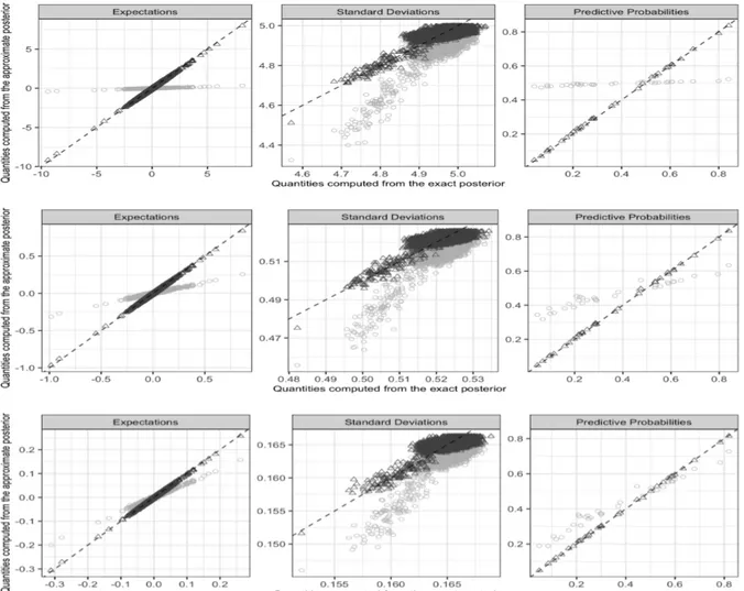
Figure 2.3: Scatterplots comparing the posterior expectations, standard deviations and predictive probabilities computed from 20000 values sampled from the exact SUN posterior, with those provided by the mf-vb (light grey circles) and pfm-vb (dark grey triangles). Each row represents a different scenario, respectively ν2

p = 25, 25 · 100/p, 25 · 10/p.

under mf-vb and pfm-vb. As is clear from Figure 2.2, pfm-vb produces approximations which perfectly overlaps with the exact posterior in all cases, including also the worst-case scenario with the highest Wasserstein distance. Consistent with Theorem 2.1, mf-vb has instead a reduced quality mostly due to a tendency to shrink, sometimes dramatically, towards zero the locations of the actual posterior. This behavior is studied more in detail in Figure 2.3, where posterior expectations and standard deviations are shown, together with the predictive probabilities for the held-out observations, for the scenarios ν2

p = 25

considered so far and also for ν2

p = 25 · 100/p and νp2 = 25 · 10/p. These two last values for

ν2

p correspond to fixing the total variance of the linear predictor as if there were

respec-tively 100 and 10 coefficients with prior standard deviation 5, in line with Gelman et al. (2008), while the others were fixed to zero. The over-shrinkage of the posterior means can be seen in the first column of Figure 2.3, which compares the posterior expectations computed from 20000 values sampled from the exact SUN posterior with those provided

(29)

by the closed-form expressions under mf-vb and pfm-vb reported in Section 2.2. We can notice that such a behavior is dramatic for the case of constant prior variance, and still remains significant when ν2

p is allowed to decrease with p. Also the standard deviations

are slightly under-estimated relative to pfm-vb that notably removes bias also in the sec-ond order moments. Consistent with the results in Figures 2.1–2.2, the slight variability of the pfm-vb estimates in the second column of Figure 2.3 is arguably due to Monte Carlo error. We conclude by assessing quality in the approximation of the exact posterior predictive probabilities for the 33 held-out individuals. These measures are fundamental for prediction and, unlike for the first two marginal moments, their evaluation depends on the behavior of the entire posterior since it relies on a non-linear mapping of a linear combination of the parameters β. In the third column of Figure 2.3, the proposed pfm-vb essentially matches the exact posterior predictive probabilities, thus providing reliable classification and uncertainty quantification. Instead, as expected from the theoretical results in Corollary 2.7, mf-vb over-shrinks these quantities towards 0.5.

2.4 Discussion and Future Research Directions

This chapter highlights notable issues in state-of-the-art methods for approximate Bayesian inference in high-dimensional binary regression, and proposes a partially factorized mean-field variational Bayes strategy which provably covers these open gaps. Our basic idea is to relax the mean-field assumption in a way which approximates more closely the fac-torization of the actual posterior, but still allows simple optimization and inference. The theoretical results confirm that the proposed strategy is an optimal solution in large p set-tings, especially when p n, and the empirical studies suggest that the theory provides useful insights also in applications not necessarily meeting the assumptions.

While our contribution provides an important advancement in a non-Gaussian regres-sion context where previously available Bayesian computational strategies are unsatisfac-tory (Chopin and Ridgway, 2017), the results in this chapter open new avenues for future research. For instance, the theoretical issues of mf-vb and map estimators presented in Section 2.2.1 for large p settings point to the need of further theoretical studies on the use of mf-vb and map estimators in high-dimensional regression with non-Gaussian responses. In these contexts, our general idea of relying on a partially factorized ap-proximating family could provide a viable strategy to solve potential issues of current approximations, as long as simple optimization is possible and the approximate poste-rior density for the global parameters can be derived in closed-form via marginalization of the local variables. This strategy could be also useful in Bayesian models relying on hierarchical priors for β that facilitate variable selection and improved shrinkage. Albeit interesting, this setting goes beyond the scope of the contribution.