Integrative modelling of the antibody antigen interactions

SAPIENZA Università di Roma PhD Programme in Life Sciences

XXXII Cycle

Integrative modelling of the antibody antigen interactions

Candidate

Francesco Ambrosetti

Supervisor

Prof. Francesca Cutruzzolà

Tutor Coordinator

“War is peace.

Freedom is slavery. Ignorance is strength.”

Abstract 5 Background 5 Aim 6 Results 6 Publications 8 1. Chapter I 9 1.1 General introduction 9 1.2 Antibody structure 11 1.3 Production of antibodies 14 1.4 Antibody numbering 17 2. Chapter II 19 2.1 Molecular docking 19

2.2 Docking of antibody-antigen complexes 21

3. Chapter III 23

3.1 Modelling of antibody-antigen complexes 23

3.2 Dataset 24

3.3 Docking scenarios 25

3.4 Docking settings 27

3.5 Docking performance 29

3.6 HADDOCK performance – Cluster based 32

3.7 Sampling performance 34

4. Chapter IV 40

4.1 proABC-2: PRediction Of AntiBody Contacts v2 and its application to information-driven docking 40 4.2 Dataset and interaction calculation 41

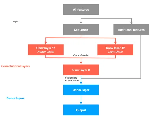
4.3 Neural network features 42

4.4 Convolutional Neural Network (CNN) 43

4.5 Model performance 45

4.6 Docking scenarios and settings 47

4.7 Prediction-driven docking accuracy 48

4.8 Web server 51

Conclusions and future perspectives 53

Abstract

Background

Over the years the use of monoclonal antibodies (mAbs) for therapeutic purposes has been experiencing a significative boost. The reasons behind this enormous growth reside in both their inherent structural properties and in technological advances for their production and characterization. Indeed, their intrinsic high affinity and specificity toward a specific antigen, together with their modular anatomy, which largely simplify their engineering, are the most important drivers of this great market expansion.

Antibody-based therapeutics are developed via well-established processes that can be broadly categorized into Lead Identification and Lead Optimization. During Lead Identification animal immunization or surface display technologies are used to generate a large number of ‘hit’ molecules which need to be further triaged. Following various rounds of screening and design during Lead Optimization, a small number of high affinity lead candidates are selected. During Lead Identification and Optimization, molecules are assessed for unfavourable characteristics such as immunogenicity or poor biophysical properties and experimental methodologies have been developed in order to improve such proprieties. A sound knowledge of the antibody binding site and the relationship between antibody and antigen residues is of paramount importance for the effective design of such strategies.

Structural experimental techniques such as Nuclear Magnetic Resonance (NMR) or X-ray crystallography can be used to study antibody-antigen interactions but they are usually expensive and time consuming and not always applicable. Therefore, the development of computational methods is offering an attractive alternative and a faster approach for the characterization of antibodies and their

strategy to elucidate the interaction between antibodies and antigens providing a tool to understand the role played by each residue in the binding.

Despite great progresses in protein-protein docking in general, modelling of antibody-antigen complexes, which is a specialized application of the broader field of molecular docking, has been demonstrated to remain challenging.

Aim

This work aimed at investigating how information about the antibody paratope and the antigen epitope can be successfully used into an information-driven docking algorithm to characterize the molecular interactions between antibodies and antigens.

In order to be able to use more accurate information about the antibody binding site, this work also aimed at improving proABC, a paratope prediction tool, and at demonstrating how this information impacts antibody-antigen molecular docking.

The overarching aim is to deepen our understanding of antibody-antigen recognition process and to provide computational tools and strategies that could facilitate antibody design and engineering.

Results

In this work I describe how information on the antibody hypervariable loops and the binding epitope can be effectively used to drive the modelling of their interaction by docking. In particular, I compare the accuracy of four docking software: ClusPro, HADDOCK, LightDock and ZDOCK in predicting antibody-antigen complexes. HADDOCK, which applies a purely data-driven strategy, performs better than the other systems especially when information about the epitope is provided.

I also investigate the accuracy of HADDOCK and LightDock (the only two software which allow flexibility of the components among the tested ones) in predicting the conformational change of the H3 loop, which is crucial for the binding and notoriously challenging to model. The results, described in the related paper “Modelling

antibody-antigen complexes by information-driven docking”,

confirm that HADDOCK shows the best accuracy and that, even if to some extent it is not able to correctly model the conformation of the loop, it manages to predict the right H3 interactions with the antigen, providing valuable information for antibody engineering. To further improve the accuracy of the docking, I developed

proABC-2 (PRediction Of AntiBody Contacts v2), which is an update,

based on a deep learning framework, of the algorithm implemented in proABC originally developed by Olimpieri and co-workers (Olimpieri et al., 2013). The method is able to accurately predict the specific paratope residues and the type of interaction, starting from the antibody sequence alone and without additional information about the antigen. I demonstrate how its predictions can be effectively used to drive the docking using HADDOCK in order to improve its modelling accuracy. proABC-2 is freely available and accessible for academic purposes as a web server.

Publications

Miotto, M., Olimpieri, P.P., Di Rienzo, L., Ambrosetti, F., Corsi, P., Lepore, R., Tartaglia, G.G., and Milanetti, E. (2019). Insights on protein thermal stability: a graph representation of molecular interactions. Bioinformatics 35, 2569–2577.

Koukos, P.I., Roel-Touris, J., Ambrosetti, F., Geng, C., Schaarschmidt, J., Trellet, M.E., Melquiond, A.S.J., Xue, L.C., Honorato, R.V., Moreira, I., Kurkcuoglu, Z., Vangone A., and Bonvin, A.M.J.J. (2019). An overview of data-driven HADDOCK strategies in CAPRI rounds 38-45. BioRxiv 10.1101/718122v1. Norman, R.A., Ambrosetti, F., Bonvin, A.M.J.J., Colwell, L.J., Kelm, S., Kumar, S., and Krawczyk, K. (2019). Computational approaches to therapeutic antibody design: established methods and emerging trends. Brief. Bioinform. Advanced Online Publication.

Ambrosetti, F., Jiménez-García, B., Roel-Touris, J. and Bonvin,

A.M.J.J. (2019). Modelling antibody-antigen complexes by information-driven docking. Structure, Advanced Online Publication (2019).

Ambrosetti, F., Olsen, T.H., Olimpieri, P.P., Jiménez-García, B.,

Milanetti E., Marcatilli, P. and Bonvin, A.M.J.J. (2019). proABC-2: PRediction Of AntiBody Contacts v2 and its application to information-driven docking. Manuscript in preparation

1. Chapter I

1.1 General introduction

Our ability to survive even in very unfavourable environments relies on the capacity of our organism to adapt itself according to the external conditions. To achieve this degree of flexibility different systems are finely tuned with one of the most important ones being known as the immune system. It allows us to fight and defend ourselves against pathogens and infections, being able to distinguish between “self” and “non self”. Two main responses are used by the immune system to fight extraneous attacks: innate and adaptative. As suggested by the names, the former refers to all of those mechanisms that are innately present to fight different ranges of threats, while the latter consists of all of the specific strategies developed by the organism upon interaction with a given pathogen. The innate system is designed to directly react to a threat, while the adaptive one requires some time to generate and fine tune the protective response. Antibodies (or immunoglobulins) are the result of this adaptive strategy and their role is crucial in order to identify and neutralize foreign organisms by recognizing specific antigens.

The ability of antibodies to recognize and bind with high affinity and specificity a given antigen, along with their highly modular anatomy which largely facilitate their engineering and design, makes them valuable weapons to fight against specific diseases. Therefore, since

their discovery in the 20th _{century by Paul Ehrlich they attracted the}

attention of researchers and industries in a wide range of different applications.

Nowadays immunoglobulins have revolutionized the medicine with more than 570 antibody therapeutics studied at various clinical phases in 2019, five of the top selling blockbusters are monoclonal antibodies (mAbs) and their market presence is expanding (Kaplon and Reichert, 2019). This rising trend in the use of antibodies for therapeutic purposes mainly relies on faster and more efficient design strategies to study and characterize them. Along with this, the development of in vitro phage display technologies and the generation of transgenic mice expressing human antibodies has considerably boosted and facilitated the production of highly specific antibodies (Larrick et al., 2016).

Over the years, experimental techniques have been developed and optimized in order to get insights into immunoglobulin structures and properties. However, often such experimental methodologies are expensive and time-consuming. Computational approaches are providing a valuable alternative to standard experimental methods, allowing faster, easier and cheaper characterization of immunoglobulins and the way they interact with their cognate antigen. One major driver of this shift is the increasing number of sequence and structural data which is paving the way for the improvement of computational methods in order to increase their accuracy and reliability.

Despite these developments, current computational approaches, as will be discussed in the following chapters, still show limitations due to the inherent properties of antibodies and several challenges (e.g. the prediction of the antibody antigen complexes and the modelling of the H3 loop) that still need to be overcome. Therefore, new approaches are required to tackle these problems taking advantage from the large amount of data presently available.

1.2 Antibody structure

Antibodies, or Immunoglobulins (Ig), are “Y-shaped” globular proteins produced in jawed vertebrates by B-cells in response to an external threat for the organism. Most of the times they are composed of two couples of identical polypeptide chains named heavy (H) and light (L) chain, kept together by disulphide bonds. In humans, the H and L chains can naturally assemble into five isotypes: IgG, IgD, IgE (monomeric forms), IgA (dimers) and IgM (pentamers) according to

their heavy chain class, respectively: g, d, e, a or µ. For the light

chain, there are four different isotypes but only two of them are present in mammals: k and l (Schroeder and Cavacini, 2010).

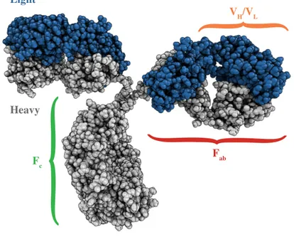
Antibodies consist of one crystallizable (Fc) and two antigen binding

(Fab) fragments as illustrated in Figure 1. The Fab domain contains the

heavy and light variable segments (VH and VL) which are the regions

involved in the recognition of the antigen. The VH and VL domains

show very high sequence and structural variability among the antibody repertoire. In particular, both heavy and light chain variable segments contain three regions where the sequence displays the highest variability. These regions are known with the name of

Complementarity Determining Regions (CDRs). The remaining part

of the variable domain is called Framework and is characterized by a high sequence conservation. Its tertiary structure consists of a 2-layer sandwich of 7-9 antiparallel β-strands arranged in two β-sheets forming the so-called immunoglobulin-like fold.

Francesco Ambrosetti

Figure 1: View of an immunoglobulin structure (PDB code: 1IGT). The two heavy

chains are shown in grey while the light ones are represented in blue. The variable (VH/VL) domain and the binding (Fab) and crystallizable (Fc) fragments, are highlighted in orange, red and green, respectively.

Each CDR harbours one loop, also named hyper variable loop (HV), for a total of six loops, three for the heavy chain (H1, H2, H3) and three for the light chain (L1, L2, L3) (Te Wu and Kabat, 1970). They play a crucial role in the binding of the antigen (Novotný et al., 1983). Despite their intrinsic high sequence variability, as demonstrated by Chothia and co-workers (Chothia et al., 1989), five out of the six HV loops exhibit a small set of well-defined conformations according to the length and to the presence of specific residues located in key positions of the antibody variable domain.

{

{

{

H3 is the loop which shows the highest structural and sequence diversity and it is also the one that is mainly involved in the antigen recognition (Shirai et al., 1996; Weitzner et al., 2015). Its modelling is one of the main challenges in the antibody modelling field. Structurally, is divided into two regions called “torso” and “apex” respectively more proximal or distal to the antibody framework. While for the apex it is not possible to define any “canonical conformation”, the torso can be classified into “bulged” on “non

bulged” depending on the presence and absence of arginine and

1.3 Production of antibodies

Production of antibodies is a complex and very well-regulated procedure. Indeed, the immune system has to be ready to fight with high specificity against a huge range of external (virus, bacteria, parasites) and internal threats (cancer cells). To do that the organism must be able to generate billions of different B-cells capable of releasing antibodies in response to a particular antigen. It has been

estimated that around 5x109 _{B-cells are present in an organism}

(Briney et al., 2019) producing distinct B-cell receptors (membrane or bound) or antibodies (in soluble form). The mechanism that underlies the generation of a such large volume of immunoglobulins based on the limited genomic space involves the somatic recombination of different gene segments, namely: variable (V), diversity (D), joining (J) and constant (C) segments. The overall process is known with the name of V(D)J recombination (Hesslein and Schatz, 2001; Tonegawa, 1983).

These genomic segments are present in clusters and located in different loci situated in different chromosomes. In total in the human organism it is possible to find three different loci: one for the heavy chain, one for the isotype l of the light chain and one for the k one (Bassing et al., 2002).

The heavy chain locus shows in sequence the V, D and J segments followed by the C one. The segments V, D and J encode for the entire variable domain of the heavy chain while the C segment is responsible for the constant domain, therefore it defines the immunoglobulin class. The two loci for the light chain include a group of V segments followed by the J ones. They are responsible for the first and last part of the light chain variable domain. The position of the C segments is different depending on the specific light chain

segments while in the case of kappa the C segments are alternated with the J ones.

The V(D)J recombination occurs together with the maturation of the B-cell. It starts when a specific protein complex called V(D)J

recombinase recognizes conserved regions named recombination signal sequences (RSS) surrounding two D and J segments on the

heavy chain locus. This recognition leads to the formation of a ring structure in which a D and J segment are close to each other. Then the V(D)J recombinase cleaves and joins together two random D and J segments. This process is not accurate, with some nucleotides being added or deleted, and largely contributes to the final variability of the antibody repertoire.

After the DJ recombination the two segments now joined together are successively combined to a random V segment leading to the formation of the so-called germline sequence (IGHV) which encodes for the full variable domain of the immunoglobulin heavy chain. Finally, the splicing of the corresponding RNA transcript assembles together the VDJ segment and the C one resulting in the final generation of the full functional heavy chain (Schatz and Swanson, 2011).

Once the heavy chain assembling is completed the rearrangement of the light chain can take place following similar steps.

The V(D)J recombination process is already able to introduce some level of variability in the generation of the immunoglobulins. However, it is not able on its own to explain the huge variety of the antibody repertoire. Indeed, upon antigen exposure, the antibody-producing B-cells undergo a natural process of affinity maturation, based on somatic hypermutation (Peters and Storb, 1996). This process introduces mutations primarily in the CDR regions and in the HV loops developing a specific and high-affinity binder. Together with the diversity introduced by V(D)J recombination, somatic

hypermutation can produce an estimated 1012_-1015 _{possible antibody}

sequences (Glanville et al., 2009) increasing the probability of recognizing an arbitrary foreign antigen.

1.4 Antibody numbering

In order to study immunoglobulins on a large scale it is necessary to map the antibody sequence onto a standardized framework to allow the unambiguous identification of residues which show equivalent structural position by assigning a unique identifier to the amino acids of the variable domain. This is particularly relevant given the high similarities between antibody sequences and the presence of conserved residues in specific key positions. The numbering schemes contextualize each position within the structure of an antibody, allowing for rapid delineation of CDRs and framework regions. Since the seminal work to define a standard numbering scheme for antibodies was carried out by Kabat in 1970 (Te Wu and Kabat, 1970), the Chothia (Chothia and Lesk, 1987) and IMGT (international ImMunoGeneTics information system) (Lefranc, 2011) schemes have been adopted as the main alternatives. Additional numbering schemes such as Contact (MacCallum et al., 1996), North (North et al., 2011), WolfGuy (Bujotzek et al., 2015) and Aho (Honegger and Plückthun, 2001) exist but these are less prevalent.

Kabat and IMGT definitions are based on sequence alignments identifying conserved positions in the variable region whereas Chothia, which is a modification of the first Kabat scheme, takes into account the 3D structure of the CDR loops.

In this work we are following the Chothia numbering scheme. More specifically, it assigns a consecutive number to all the framework residues of the light and heavy variable domain up to the ones that are part of one HV loop. From them, it continues by adding to the number of the last framework residues a letter (which identifies an insertion) until the end of the loop, then the consecutive numbering starts again (see Figure 2).

There are three freely available software packages to perform numbering of antibodies; ANARCI (Dunbar and Deane, 2016), Abnum (Abhinandan and Martin, 2008) and AbRSA (Li et al., 2019), to act as the first step in computational antibody analysis.

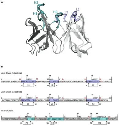
Figure 2: (A) View of the variable domain of an antibody. CDRs are highlighted.

(B) Chothia numbering scheme for the heavy and light chain (k and l isotypes). Arrows represent the hypervariable loops. In violet and cyan are represented the CDRs of the light and heavy chain, respectively. Framework residues are coloured in white and grey for the light and heavy chain respectively. Conserved residues are reported in red.

Figure from: PIGSPro: Prediction of immunoGlobulin structures v2. Nucleic Acids

2. Chapter II

2.1 Molecular docking

Characterization of the interface between two molecules is a key step in order to elaborate efficient and effective rational design strategies for therapeutics. Several experimental techniques can be used to determine the three-dimensional (3D) structure of molecular complexes. These methods include X-ray crystallography, Nuclear Magnetic Resonance (NMR) and Cryo-Electron Microscopy (Cryo-EM). Despite their reliability and accuracy, experimental methods are generally time consuming and expensive. Therefore, computational approaches can provide a valuable, more rapid solution to gain information about the interacting residues of two molecules.

In this scenario, one suitable approach is “molecular docking”. It can be defined as the process that, starting from the free form structures of the components, predicts the structure of the complex. It usually involves two different steps: the sampling step, during which thousands of possible complex conformations are generated, and the

scoring step, in which the conformations are ranked according to a

specific scoring function to identify models which are closer to the native conformation.

According to the sampling strategy used during the simulation, docking methods can be classified into two categories. The first class includes algorithms which perform a global search around the entire surface of the components without taking into account any information about the binding region (ab initio docking). The second class consists of docking methods that can use experimental data, for example coming from hydrogen-deuterium exchange (HDX) coupled with mass spectrometry, from mutational studies (Sevy et

al., 2013), or from predicted information about the binding interface to drive the sampling during docking (information-driven, local or

integrative docking) (Rodrigues and Bonvin, 2014). Both classes can

benefit from available information during the scoring step to select models that are consistent with the available information about the interaction.

Most protein-protein docking algorithms do not consider possible conformational changes occurring upon binding (rigid-body docking). This is the case for software such as ClusPro (Kozakov et al., 2017) and ZDOCK (Chen and Weng, 2002) that are based on the Fast Fourier Transform (FTT) search algorithm (Katchalski-Katzir et al., 1992). In most cases, however, protein flexibility is a crucial factor to be considered (Kotev et al., 2016). Approaches that allow for flexibility of side chains and/or backbone have also been developed such as ATTRACT (De Vries et al., 2015), LightDock (Jiménez-García et al., 2018), Swarmdock (Torchala et al., 2013) SnugDock (Sircar and Gray, 2010) and HADDOCK (De Vries et al., 2010). The former three do that by using normal modes, the latter two by allowing some flexibility along side-chains and backbone during a refinement stage.

The performance of various docking software is regularly assessed by the Critical Assessment of Predicted Interactions (CAPRI) experiment (Méndez et al., 2003), catalysing the effort of researchers towards the development of new and more accurate methods.

2.2 Docking of antibody-antigen complexes

The possibility to provide information either at the sampling and/or at the scoring level is particularly relevant in the case of antibody-antigen docking as CDRs and in particular the HV loops offer a reasonable proxy of the binding interface on the antibody. In fact, some docking methods such as for example ClusPro and PatchDock (Comeau et al., 2004; Schneidman-Duhovny et al., 2005) are able to automatically define the antibody CDRs in order to use this information during the docking process.

Despite great progresses in predicting protein-protein complexes, docking of antibody-antigen complexes remains challenging (Pedotti et al., 2011; Ponomarenko and Bourne, 2007; Vajda, 2005) due to the specific properties of their interfaces (Conte et al., 1999; Sela-Culang et al., 2013).

Understanding the structural basis of the antibody-antigen interaction would pave the way to the design of new efficient biological drugs (Lippow et al., 2007). For the antibody, the residues involved in the binding – the so called paratope residues – can be predicted quite accurately through various computational approaches (Krawczyk et al., 2013; Kunik et al., 2012; Liberis et al., 2018; Olimpieri et al., 2013). The information provided by those methods has been demonstrated to be valuable to drive the docking (Liberis et al., 2018).

The identification or prediction of the set of antigen residues that are recognized by the antibody is however the most challenging part. Several methods have been reported (Ansari and Raghava, 2010; Jespersen et al., 2017; Krawczyk et al., 2014; Kringelum et al., 2012; Liang et al., 2010; Qi et al., 2014; Rubinstein et al., 2009; Sela-Culang et al., 2015), but existing epitope prediction systems still do

not provide reliable results, limiting their applicability in molecular docking (Ponomarenko and Bourne, 2007). In this context, docking approaches could present a valuable alternative to the available epitope prediction methods provided that near-native solutions can be generated and recognized. Additionally, docking approaches can elucidate the relationship between antibody and antigen residues facilitating the rational design and engineering of immunoglobulins.

3. Chapter III

3.1 Modelling of antibody-antigen complexes

In this chapter I present an assessment of the performance of ClusPro (Comeau et al., 2004; Kozakov et al., 2017), HADDOCK (De Vries et al., 2010), LightDock (Jiménez-García et al., 2018) and ZDOCK (Pierce et al., 2011) in predicting antibody-antigen structures. All those software allow to use in various ways a-priori knowledge, e.g. the hyper variable loops, into the modelling process to drive or limit the sampling and/or score the docking models.

ClusPro and ZDOCK are based on the Fast Fourier Transform (FTT), they treat the molecules as rigid systems and thus they are unable to account for conformational changes upon binding. On the other hand, LightDock and HADDOCK allow for flexibility during the simulation, the former by using normal modes, the latter by allowing motions of both side chain and backbone during a refinement stage.

3.2 Dataset

The dataset used in this work includes 16 complexes (see Table 1), all with available unbound structures, which represent the new antibody-antigen entries of the protein-protein benchmark version 5.0 (Vreven et al., 2015). These were selected because none were used for training/scoring optimization of any of the docking software considered in this work. Only the antibody variable domain was used for the docking. Antibodies and antigens were each randomly translated and rotated in order to avoid any bias related to the starting orientation (this is required since the structures in the docking benchmark are pre-oriented onto their reference bound complex). The structures were renumbered using a consecutive numbering as not all the software used in this work are able to deal with the insertion format of the Chothia scheme.

Table 1: Summary of the structures used in this work. i-RMSD(Å) indicates the

interface root mean square deviation of the Ca atoms of the interface residues calculated after finding the best superposition of bound and unbound interfaces. Complexes are grouped into two classes: Rigid and Medium according to the i-RMSD and the faction of non-native residue contacts (not reported).

Complex PDB ID 1 Protein 1 PDB ID 2 Protein 2 i-RMSD (Å)

Rigid

2VXT 2VXU Murine reference antibody 125-2H FAB 1J0S Interleukin-18 1.33

2W9E 2W9D ICSM 18 FAB fragment 1QM1 Prion protein fragment 1.13

3EOA 3EO9 Efalizumab FAB fragment 3F74 Integrin alpha-L I domain 0.39

3HMX 3HMW Ustekinumab FAB 1F45 Interleukin-12 0.73

3MXW 3MXV Anti-Shh 5E1 chimera FAB fragment 3M1N Sonic Hedgehog N-terminal domain 0.48

3RVW 3RVT 4C1 FAB 3F5V DER P 1 allergen 0.5

4DN4 4DN3 CNTO888 FAB 1DOL MCP-1 0.81

4FQI 4FQH CR9114 FAB 2FK0 H5N1 influenza virus hemagglutinin 1.08

4G6J 4G5Z Canakinumab antibody fragment 4I1B Interleukin-1 beta 0.61

4G6M 4G6K Gevokizumab antibody fragment 4I1B Interleukin-1 beta 0.49

4GXU 4GXV 1F1 antibody 1RUZ 1918 H1 Hemagglutinin 0.78

Medium

3EO1 3EO0 GC-1008 FAB fragment 1TGJ Transforming Growth Factor-Beta 3 1.37

3G6D 3G6A CNTO607 FAB 1IK0 Interleukin-13 1.86

3HI6 3HI5 AL-57 FAB fragment 1MJN Integrin alpha-L I domain 1.65

3.3 Docking scenarios

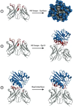
Antibody-antigen docking was performed by providing specific options for the antibody antigen-modelling. Indeed, while for the antibody the HV loops provide a valuable proxy of the binding region, as already mentioned, the definition of the antigen epitope is challenging. Therefore, I elaborated three different scenarios in order to mimic different levels of available information about the binding interface on the antigen (see Figure 3):

1. The first scenario (HV – Surf) includes information about the antibody HV loops, defined according to the Chothia numbering scheme (Al-Lazikani et al., 1997) but no information about the epitope. For HADDOCK this was complemented by all solvent-exposed antigen residues defined by selecting those with a relative accessible surface area (RSA) ≥ 40% as calculated with NACCESS (Hubbard SJ, 1993).

2. In the second scenario (HV – Epi 9) a vague definition of the epitope is provided based on all residues having any atom within 9Å from any atom of the antibody in the reference structure.

3. The third scenario (Real interface) represents the ideal case where both interfaces are well characterized. All interface residues, selected using a distance cutoff of 4.5Å between any antibody and antigen atom, were given to the docking software.

This information was used differently in the various docking software depending on their ability to deal with it. In short, HADDOCK follows a data-driven sampling strategy in which the information is encoded into ambiguous restraints to drive the

docking; LightDock uses the information both to limit the sampling to specific regions and in scoring, while ClusPro and ZDOCK include this information into their scoring functions in order to select the correct models.

Figure 3: Summary of the three docking scenarios used in this work. The first case

represents the situation in which no previous information about the epitope is known so the docking is performed exploring the whole surface of the antigen while for the antibody the HV loops are provided. In the second scenario the antibody HV loops and a loose epitope definition corresponding to the antigen residues within 9Å from the antibody are used to drive the docking. Finally, in the third scenario the real interfaces of both the antigen and the antibody (defined at

HV loops - Surface HV loops - Epi 9 Real interface 2 3 1

3.4 Docking settings

Four docking methods were compared in this work: ClusPro (Kozakov et al., 2017), HADDOCK (De Vries et al., 2010), LightDock (Jiménez-García et al., 2019) and ZDOCK (Pierce et al., 2011).

The ClusPro web server (https://cluspro.org) was used in the

Antibody Mode (Brenke et al., 2012) using default settings. Information was provided in the form of attractive residues.

ZDOCK predictions were obtained using a local installation of version 3.0.2. The sampling was set to 2000 models. ZDOCK allows the user to assign a highly unfavourable contact energy to the residues which are known not to be involved in the binding. Accordingly, all residues not included in the defined interfaces were blocked.

For LightDock I used release 0.5.6 of the software (Jiménez-García et al., 2019), which provides a mechanism for including residue restraints. At the receptor level, the surface swarms used at the start of the simulations are filtered according to the Euclidean distance of the restraints on the provided receptor residues. Only the ten closest swarms for each receptor residue restraint are kept. An additional energy term is added to the scoring function used in this work, DFIRE (Zhou and Zhou, 2009), that accounts for the percentage of satisfied restraints. The predictions are filtered with a minimum 40% cutoff of satisfied restraints, at both receptor and ligand levels. For the remaining parameters default settings were used: Anisotropic Network Model (ANM) enabled (10 first non-trivial modes for both receptor and ligand), 400 swarms before filtering by restraints, 200 glowworms per swarm and 100 simulation steps.

except that the rigid-body (it0) sampling was increased to 5000 models for the HV – Epi9 and the Real interface runs and to 10000 for the HV – Surf scenario (default is 1000). The flexible (it1) and water refinement sampling were set to 400 models for all scenarios (default is 200) (Dominguez et al., 2003). This corresponds to an increased sampling compared to the default settings. In general, the least information is available to drive the docking in HADDOCK the larger the sampling should be. The docking was performed using the

web server version of HADDOCK (https://haddock.science.uu.nl)

(Van Zundert et al., 2016). In the case of the Real interface scenario, the random removal of restraints (by default 50% of restraints are randomly discarded for each docking trial) was turned off. The information about the binding interface was encoded in the form of active and passive residues. The antibody HV loops and paratope residues were provided as active, while, for the antigen, the surface and the epitope residues, selected using a 9Å cutoff, were defined as passive. For the third, ideal scenario, the true interface epitope residues selected at 4.5Å distance cutoff were classified as active. The distinction between active and passive means that an active residue not at the interface (defined as the union of active and passive residues of the partner molecule) will result in an energy penalty while this is not the case for passive residues.

In all the methods, the antibody was treated as the receptor partner and the antigen as ligand.

3.5 Docking performance

I analysed the performance of the four docking methods in predicting antibody-antigen complexes in terms of success rate calculated as the percentage of cases in which at least one acceptable, medium or high-quality model is found in the top N ranked solutions. The model quality was defined according to the CAPRI criteria (Méndez et al., 2003). Those are based on three parameters; briefly:

1. Interface root mean square deviation (i-RMSD): calculated on the backbone atoms of all interface residues of the native complex defined using a 10Å cutoff.

2. Ligand root mean square deviation (L-RMSD): calculated by superimposing on the backbone atoms of the antibody and calculating the RMSD of the antigen backbone atoms.

3. Fraction of native contacts (Fnat): number of native contacts

in a docking model divided by the total number of contacts in the reference structure. These are defined using a 5Å cutoff. The ranges used to define the classes are shown in Table 2.

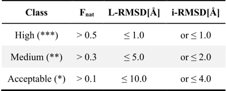
Table 2: Classification of docking models in the classes: ***, **, * according to

Fnat, and either L-RMSD or i-RMSD measures.

Class Fnat L-RMSD[Å] i-RMSD[Å]

High (***) > 0.5 ≤ 1.0 or ≤ 1.0

Medium (**) > 0.3 ≤ 5.0 or ≤ 2.0

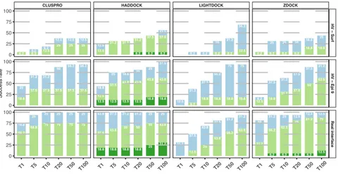
The success rate for top 1, 5, 10, 20, 50 and 100 is shown in Figure 4 for each docking method and scenario as described in the paragraph 3.3. The first panel refers to the HV – Surf scenario, the second to the HV – Epi 9 one and finally the third shows the success rate obtained using the real interface information in the docking. The latter represents the gold standard achievable by each docking approach, i.e. the best accuracy that can be reached for this dataset given a perfect interface definition (but no specific contacts) and starting from the unbound structures of the components.

Figure 4: ClusPro, HADDOCK, LightDock and ZDOCK success rate for the three

scenarios described in this work as a function of the top 1, 5, 10, 20, 50 and 100 ranked models. The top row (HV - Surf) shows the success rate using the antibody HV loops and the entire antigen surface as restraints. The second represents the success rate achieved by driving the docking with the antibody HV loops and a loose epitope definition using a 9Å cutoff. The third panel shows the docking results using the true interfaces (defined at 4.5Å). The colour coding indicates the quality of the models according to CAPRI criteria.

In the absence of any kind of information about the epitope (HV loops – surface – top row in Figure 4) the overall performance is rather low for all methods. HADDOCK reaches a success rate of 25%

0 6.2 0 6.2 6.2 0 12.56.2 0 25 12.5 0 25 12.5 0 25 12.5 0 18.8 25 0 37.5 31.2 0 37.5 31.2 0 37.5 50 0 37.5 56.2 0 37.5 56.2 0 56.2 18.8 0 68.8 25 0 75 25 0 75 25 0 75 25 0 75 25 0 12.5 12.5 0 31.2 0 31.2 6.2 31.2 6.2 37.5 6.2 37.5 12.5 12.5 12.5 18.8 12.5 37.5 25 12.5 43.8 18.8 12.5 43.8 25 18.8 43.8 25 18.8 43.8 37.5 18.8 37.5 43.8 18.8 43.8 37.5 18.8 50 31.2 18.8 50 31.2 25 50 25 31.2 43.8 25 0 6.20 6.20 6.20 25 0 6.2 31.2 0 12.5 56.2 0 12.5 0 6.2 31.2 0 18.8 37.5 0 18.8 56.2 0 18.8 75 0 18.8 75 0 31.2 0 12.5 37.5 0 25 43.8 0 43.8 37.5 0 56.2 31.2 0 62.5 31.2 0 6.2 0 6.2 25 0 6.2 25 0 6.2 25 0 18.8 18.8 0 18.8 25 0 12.56.2 0 18.8 37.5 0 31.2 31.2 0 37.5 37.5 0 50 37.5 0 62.5 31.2 0 31.2 50 6.2 56.2 31.2 6.2 62.5 25 6.2 75 12.5 6.2 81.2 12.5 12.5 75 12.5

CLUSPRO HADDOCK LIGHTDOCK ZDOCK

HV − Surf HV − Epi 9 Real interface T1 T5 T10 T20 T50 T100 T1 T5 T10 T20 T50 T100 T1 T5 T10 T20 T50 T100 T1 T5 T10 T20 T50 T100 0 25 50 75 100 0 25 50 75 100 0 25 50 75 100 Success r ate

and LightDock (0%). Note that considering the limited size of the benchmark, a difference of 6.2% only corresponds to one more successfully predicted complex. The differences are smaller for the top 10 (the typical number of models evaluated in CAPRI), with HADDOCK and ZDOCK leading with 31.2%, followed by ClusPro with 18.7%. Considering the top 100, in this scenario LightDock outperforms the other methods with a success rate of 68.7%. This is linked to the fact that LightDock is based on a very effective sampling strategy, but the scoring function used is not accurate for this type of complexes.

By providing a low accuracy definition of the epitope region (HV – Epi 9, middle row in Figure 4) the success rate increases significantly. For example, HADDOCK and ClusPro are able to predict correct models respectively for 75% and 68.7% of the cases already in the top 5 (43.8% in the top1 for both), followed by ZDOCK (56.3%) and LightDock (37.4%).

The bottom row in Figure 4 (Real interface) shows the results when both interfaces are perfectly characterized such that the exact residues involved in the binding are used in the docking. In this case HADDOCK ranks acceptable models in the top 1 position for all 16 complexes of the dataset (100% success rate), while ZDOCK, ClusPro and LightDock reach success rates of 81.2%, 75% and 31.2%, respectively.

Overall, Figure 4 shows that HADDOCK is performing best in every scenario. Even in the cases where ClusPro, LightDock and ZDOCK are able to reach comparable results (e.g. top 50 HV – Epi 9 scenario) the quality of the generated models is usually not as good as those produced by HADDOCK. This can be attributed to the different strategies of using information between those software, with HADDOCK directly using restraints during the sampling/refinement stages, and not only for filtering and/or scoring as is the case in the other software.

3.6 HADDOCK performance – Cluster based

Many approaches perform a clustering after docking in order to group together similar models and simplify the analysis. This has been demonstrated to significantly improve the accuracy of the scoring. The most widely used parameter to measure similarities among different structures is the positional RMSD. The fraction of common contacts (FCC) has been introduced as a fast and valuable alternative to classical RMSD-based methods (Rodrigues et al., 2012). FCC clustering is used by default in HADDOCK (with 4 as minimum cluster size) to cluster the docking models using a default cutoff of 0.6. This has been optimized on classical protein-protein systems. Taking into account the result of the cluster analysis it is possible to express the success rate as the percentage of cases in which there is at least one acceptable, medium or high-quality model in the top 4 cluster members of the top 1, 2, 3, 4 and 5 clusters. In this work clusters were ranked by the average HADDOCK score of their top 4 models (the default scoring scheme of the HADDOCK server (De Vries et al., 2010)). The cluster-based success rate of HADDOCK is shown in Figure 5 for the three different scenarios. Comparing Figure 4 and Figure 5, and in particular the success rate for top 1 and top 5, one can clearly see how cluster-based scoring increases the success rate of HADDOCK when information about the epitope is provided, but reduces it when no information on the antigen is available and the entire antigen surface is used to drive the docking. This is due to the fact that the sampling around the entire surface of the antigen leads to the generation of many possible different conformations. This results in many local minima of the energy landscape, which the HADDOCK scoring function is not able to distinguish properly. Also, a slightly lower number of models do fall into clusters in this case as illustrated by the clustering coverage

0.83±0.10, 0.93±0.04 and 0.99±0.003 respectively for the HV – Surf, HV – Epi 9 and the Real interface scenarios. However, even with a rather loose definition of the epitope (HV – Epi 9 scenario), clustering leads to an improvement in scoring performance from 43.8% to 56.3% for top 1. These results indicate that different scoring strategies should ideally be followed depending on the availability of epitope information or not.

Figure 5: HADDOCK cluster-based success rate for the three docking scenarios

as a function of the top 1,2,3,4 and 5 ranked clusters. The colour coding indicates the quality of the models according to CAPRI criteria.

0 12.56.2 0 18.8 0 18.8 0 25 0 25 12.5 25 18.8 12.5 37.5 25 12.5 37.5 37.5 18.8 37.5 37.5 18.8 37.5 37.5 18.8 43.8 37.5 18.8 43.8 37.5 18.8 43.8 37.5 18.8 43.8 37.5 18.8 43.8 37.5 HADDOCK HV − Surf HV − Epi 9 Real interface T1 T2 T3 T4 T5 0 25 50 75 100 0 25 50 75 100 0 25 50 75 100 Success r ate

3.7 Sampling performance

Docking involves two different steps, the sampling for the generation of thousands of models, and the scoring to select the best (near-native) models according to a specific scoring function. Most software include the information about the binding interface at the scoring stage, while HADDOCK is the only system which uses this information to drive the sampling (the information is encoded into an additional energy term that generates forces to drive the energy minimization and molecular dynamics steps). The effect of those different strategies can be noticed by calculating the number of acceptable, medium or high-quality models generated out of the total number of produced models. This number is summarized for each software in Figure 6.

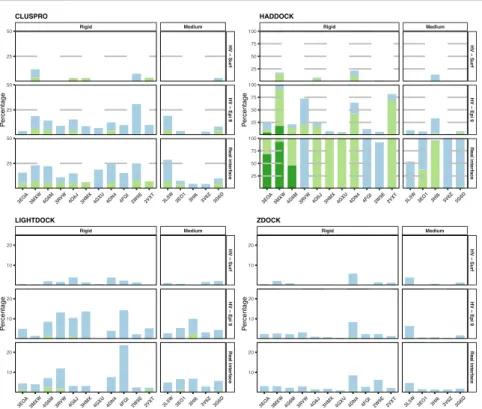
Figure 6: Percentages of acceptable, medium and high-quality models generated

by each software per complex and for each scenario. Complexes are split into rigid and medium categories according to the Docking Benchmark5 definition which is based on the size of the conformational change of the unbound molecules upon binding. Note that the Y axis scales are different for each docking method for better readability. The colour coding indicates the quality of the models according to CAPRI criteria.

One can clearly see (Figure 6) how the driving strategy implemented in HADDOCK leads to the generation of a much higher number of good models when information about the interface is provided (HV – Epi 9 and Real Interface scenarios). It has however the danger that no single acceptable model might be generated in case of bad information. The other software, ClusPro, LightDock and ZDOCK

Rigid Medium HV − Surf HV − Epi 9 Real interface 3EO A

3MXW 4G6M 3RVW4G6J 3HMX 4GXU 4DN4 4FQI 2W9E 2VXT 3L5W 3EO1 3HI6 3V6Z 3G6D 25 50 25 50 25 50 P ercentage CLUSPRO Rigid Medium HV − Surf HV − Epi 9 Real interface 3EO A

3MXW 4G6M 3RVW4G6J 3HMX 4GXU 4DN4 4FQI 2W9E 2VXT 3L5W 3EO1 3HI6 3V6Z 3G6D 25 50 75 100 25 50 75 100 25 50 75 100 P ercentage HADDOCK Rigid Medium HV − Surf HV − Epi 9 Real interface 3EO A

3MXW 4G6M 3RVW4G6J 3HMX 4GXU 4DN4 4FQI 2W9E 2VXT 3L5W 3EO1 3HI6 3V6Z 3G6D 10 20 10 20 10 20 P ercentage LIGHTDOCK Rigid Medium HV − Surf HV − Epi 9 Real interface 3EO A

3MXW 4G6M 3RVW4G6J 3HMX 4GXU 4DN4 4FQI 2W9E 2VXT 3L5W 3EO1 3HI6 3V6Z 3G6D 10 20 10 20 10 20 P ercentage ZDOCK

use the interface information only at the scoring level (except for LightDock that filters starting swarms to sample around the provided binding site). These have the advantage that they perform an exhaustive search of the interaction space, but this comes at the cost of a small number of near-native models generated. In that case, the scoring becomes crucial to identify the acceptable models.

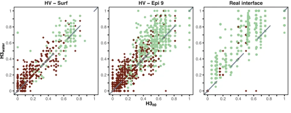
3.8 H3 loop modelling performance

The H3 loop of antibodies is the most important loop involved in antigen recognition. Its accurate modelling is still a challenge due to its high structural and sequence variability. Of the four docking software used in this work, two allow for conformational changes during the docking, namely HADDOCK and LightDock. I analysed their capability of inducing the right conformational changes of the loop upon binding with the antigen. For this I superimposed the antibody framework residues of the bound and the unbound structure

and calculated the RMSD of H3 (H3unbound). Then I repeated the same

procedure for each docking model compared to the native complex (H3model). For both HADDOCK and LightDock, models produced

from the different scenarios were merged and split into correct (i-RMSD ≤ 4Å) and wrong models (i-(i-RMSD > 4Å). Figure 7 shows the

distribution of H3model versus H3unbound for correct and wrong models.

Values below the diagonal correspond to an improvement of the conformation of the H3 loop. Overall, for HADDOCK (Figure 7A) the flexible refinement tends to increase the RMSD of the H3 loop

for complexes that show a low H3 conformational change upon

binding but, in contrast, for complexes undergoing larger

conformational changes of H3unbound, the refinement leads to

improvement in the H3 conformation, especially in the scenarios where information about the epitope is provided (HV – Epi 9 and Real interface), with a maximum observed improvement of 1.25Å. In the case of LightDock (Figure 7B) the final selected H3 loop conformation from normal modes remains very close to the unbound form with no remarkable changes in terms of RMSD.