XXV Ciclo
GEOCHRONOLOGY OF TERRACED COASTAL
DEPOSITS IN CALABRIA AND EASTERN SICILY:
TECTONIC IMPLICATIONS
Dottoressa
Gloria Maria Ristuccia
Tutor: Prof. C. Monaco
Co-tutors: Prof. S.O. Troja
Prof.ssa A.M. Gueli
"Non ho particolari doti. Sono solo appassionatamente curioso"!! (Albert Einstein)
ABSTRACT
Calabrian Arc and Eastern Sicily (Southern Italy) are characterized by flights of coastal terraces occurring in various geological domains. These features are formed by interaction between the glacio-eustatic sea level changes and Late Quaternary uplift. Indeed, since Middle Pleistocene times this region of the central Mediterranean has been mostly affected by extensional and transcurrent tectonics that have been coupled with a strong regional uplift with values of ~1 mm/yr along the Tyrrhenian and Ionian coasts. Thus, by combining ages and elevations of inner edges with the OIT stages of high sea-level stands, it is possible to accurately evaluate the uplift rates of coastal areas and to discriminate, where possible, the regional and local components of uplift. At this purpose, in this thesis the Optically Stimulated Luminescence (OSL) method has been used, mainly for its applicability to the detrital minerals of the terraced sediment (i.e. quartz) and for its accuracy. The research project is based on interdisciplinary study that involved the PH3DRA (Physics for Dating Diagnostic Dosimetry Research and Applications) laboratories of the Department of Physics and Astronomy of the Catania University, where preparation of geological samples, measurements and analysis of results were carried out, in order to optimize the dating procedure and to obtain OSL age of samples collected from the studied terraced deposits. For each sites the structural and geomorphological issues have been dealt with and then samples of sands have been collected from the studied areas. Four key sites, characterized by different tectonic setting, have been chosen: Amendolara (north-eastern Calabria), Capo Vaticano peninsula (western Calabria), Sant’Agata di Militello (north-eastern Sicily), Terreforti Hills (eastern Sicily). For the first site, the OSL dating methodology on quartz grains failed.
Quaternary terraced deposits outcropping on the Capo Vaticano peninsula have been investigated in order to obtain new chronological estimates. OSL age
provided new constraints for correlating the distinct orders of marine terraces with the last seven interglacial stages of the eustatic curve. This correlation indicates that in the Middle-Late Pleistocene this portion of the southern Calabrian Arc was affected by a vigorous uplift characterized by rates up to ~2 mm/yr, accompanied by faulting and tilting of the peninsula towards the northeast.
Along the coastal sector of Sant’Agata di Militello the geomorphological survey and the analysis of stereo-pairs of aerial photographs allowed to recognize at least five main orders of well-preserved Quaternary surfaces and relative deposits. They are mostly located on the hanging-wall and on the footwall of the Pleistocene northwest-dipping Capo d’Orlando normal fault, which controlled the geomorphological evolution of the coastal area. In order to better define the whole terrace chronology, deposit samples were analysed by OSL methodology, a conventional single-aliquot regenerative-dose (SAR) protocol used with sand-sized quartz. New dating, together with the detailed morphostructural analysis, allow to relate the 2nd and 4th order terraces to MIS 5.5 and 8.5, respectively, and to reconstruct the tectonic evolution of this coastal area, constraining the activity of the Capo d’Orlando fault.
Coastal-alluvial terraces outcropping in the area between Mt. Etna volcano and the Catania Plain, known as the “Terreforti Hills”, at the front of the Sicilian fold and thrust system, were analyzed. The obtained OSL ages were consistent with the normal evolutionary model of a terraced sequence, moving from the highest to the lowest elevations and the new data allowed us to determine a mean uplift rate of 1.2 mm/yr during the last 330 ka, mostly related to regional uplift processes coeval to Quaternary sea-level changes. Moreover, the two highest order terraces are folded, forming the large Terreforti anticline. According to our analysis, this anticline represent a thrust propagation fold developed at the front of the Sicilian chain between 236 and 197 ka ago.
I
INDEX
INTRODUCTION
CHAPTER 1–TECTONIC FRAMEWORK 1.1-GEOLOGICAL SETTING
1.2-COASTAL TERRACES AS A TOOL FOR DETERMINING VERTICAL DEFORMATION CHAPTER 2–OSL METHODOLOGY
2.1-OSL DATING: HYPOTHESIS 2.2-PRINCIPLE OSL
2.2.1-SIMPLE MODEL: ONE TRAP/ONE CENTER 2.3-OSL DECAY CURVE
2.4-NATURAL RADIOACTIVITY METHODOLOGY 2.5-SAMPLING COLLECTION
2.6-SAMPLE PREPARATION FOR OSL MEASUREMENTS 2.7-QUARTZ AS DOSIMETER
2.8-OSL MEASUREMENTS
2.8.1-SINGLE-ALIQUOT REGENERATIVE-DOSE (SAR) PROTOCOL 2.8.2-REJECTION CRITERIA
2.9-DISCUSSION OF DATING RESULTS: ANALYSIS OF DE DISTRIBUTION AND STATISTICAL MODEL 2.10-DOSE RATE DETERMINATION
2.10.1-RADIOACTIVE DISEQUILIBRIUM
CHAPTER 3 – LUMINESCENCE CHRONOLOGY OF PLEISTOCENE MARINE TERRACES OF CAPO VATICANO PENINSULA (CALABRIA, SOUTHERN ITALY)
3.1-INTRODUCTION
3.2-GEOLOGICAL AND GEOMORPHOLOGICAL SETTING 3.3-OSL MEASUREMENTS
3.4-AGE RESULTS AND CORRELATIONS 3.5-DISCUSSION
3.6-CONCLUSIONS
CHAPTER 4–MIDDLE-LATE PLEISTOCENE MARINE TERRACES AND FAULT ACTIVITY IN THE SANT’AGATA DI MILITELLO COASTAL AREA (NORTH-EASTERN SICILY)
4.1-INTRODUCTION 4.2-GEOLOGICAL SETTING
4.3-MARINE TERRACES ALONG THE SANT’AGATA DI MILITELLO 4.4-LUMINESCENCE DATING
4.4.1-SAMPLE COLLECTION AND PREPARATION 4.4.2-MEASUREMENTS AND RESULTS
II 4.5-AGE RESULTS, CORRELATIONS AND DEFORMATION PATTERN
4.6-CONCLUSIONS
CHAPTER 5–OSL CHRONOLOGY OF QUATERNARY TERRACED DEPOSITS OUTCROPPING BETWEEN MT. ETNA VOLCANO AND THE CATANIA PLAIN (SICILY, SOUTHERN ITALY)
5.1-INTRODUCTION 5.2-GEOLOGICAL SETTING
5.3-STRATIGRAPHICAL AND GEOMORPHOLOGICAL FEATURES 5.4-OSL DATING
5.4.1-EXPERIMENTAL DETAILS
5.4.2-SINGLE GRAIN DE DISTRIBUTION AND BLEACHING
5.5-AGE RESULTS, CORRELATIONS AND GEODYNAMIC CORRELATIONS 5.6-CONCLUSIONS
CONCLUSION
APPENDIX A– INSTRUMENTATION
1
INTRODUCTION
Calabrian Arc and Eastern Sicily (Southern Italy) are regions of the central Mediterranean where the effects of Quaternary tectonic events are well preserved.
Since Middle Pleistocene times, tectonic processes have been coupled with a strong regional uplift with values of ~1 mm/yr along the Tyrrhenian and Ionian coasts (Westaway, 1993; Bordoni and Valensise, 1999; Bianca et al., 1999; Catalano et al., 2003). Late Quaternary uplift, associated with the glacio-eustatic sea level changes, described by the global eustatic curve of Waelbroeck et al. (2002), caused the development of prominent flights of coastal terraces that represent a peculiar morphological feature of this area (Valensise and Pantosti, 1992; Westaway, 1993; Bianca et al., 1999; Catalano and De Guidi, 2003; Catalano et al., 2003; Tortorici et al., 2003). Coastal terraces originated from vertical displacement above sea level (a.s.l.) of erosional or depositional surfaces formed during a relative sea-level stand with their inner edges (i.e. a palaeoshoreline). They mostly represent the morphological record of one of the relative maximum high-stands reached by the sea level during a main interglacial stage (Bloom et al., 1974). Considering ~130 m of utmost Pleistocene-Holocene eustatic oscillations (Shackleton and Opdyke, 1973; Chappell and Shackleton, 1986; Lajoie, 1986; Pirazzoli, 1991; Westaway, 1993) and that the present-day sea level is very close to the Quaternary maximum (Chappell and Shackleton, 1986; Pirazzoli and Suter, 1986; Muhs, 1992; Westaway, 1993), the presence of coastal terraces several hundred metres above sea level indicates tectonic uplift. Thus, the reconstruction of the elevation changes of a raised palaeoshoreline is helpful in evaluating the amount of tectonic deformation of a region. Moreover, the elevation of terraces and their offset across the main faults could be used to establish the relative contribution of regional and fault-related
2
sources to uplift. Hence the chronological datum of terrace formation appears of primary importance, because their dating should provide an understanding of past sea level fluctuations, which are interlinked with global climate changes and/or local tectonic movements. As regards the geochronology, there are a few direct dating methods which can establish the time of deposition of sediments. These methods (e.g. radiocarbon, U-series, Electron Spin Resonance, Amino-Acid Racemization, ...) are all applied to fossil shells and restricted to fossiliferous marine terraces. Their accuracy may be hampered by the poor preservation of the marine fauna (molluscs and corals) or the presence of untraceable reworked shells. These difficulties will be overcome by the use of an independent dating technique, such as the Optically Stimulated Luminescence (OSL) method (Huntley et al., 1985; Aitken, 1998), whose applicability is turned to detrital minerals of the terraced sediment itself (i.e. quartz and feldspars).
In this thesis, an interdisciplinary study has been carried out in order to accurately date flights of Quaternary terraces located in key areas of the Calabrian Arc and eastern Sicily (Fig. 1) and evaluate the vertical deformation rates, both local and regional, of the coastal areas where they are located. In fact, the research project involved the PH3DRA (Physics for Dating Diagnostic Dosimetry Research and Applications) laboratories of the Department of Physics and Astronomy of the Catania University, where preparation of geological samples (based on mineralogical composition), measurements (based on physical behaviour of mineral) and analysis of results (based on the dating model) were carried out, in order to obtain OSL dating of samples collected from the studied terraced sequences.
The thesis starts (Chapter 1) with the description of the geological setting of the studied areas and of the coastal terraces as a tool for determining vertical
3
deformation. In fact, comparing the altitude distribution of inner edge of coastal terraces with available absolute dating results, the pattern of the regional signal of uplift can be reconstructed.
Chapter 2 treats the basic principles of the OSL methodology, the hypothesis of applicability, and some tests that minimize all the issues regarding the geological dating of samples. The application of modified single-aliquot regeneration dose (SAR) protocol (Murray and Wintle, 2000, 2003) to sand grained quartz, both to the small aliquot and single grain, to determinate the equivalent dose (De), are then
investigated.
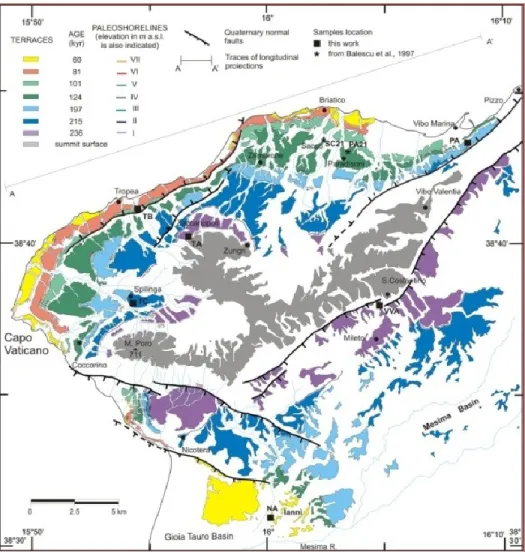
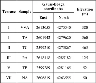
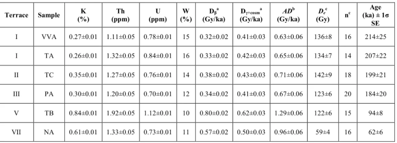
In Chapter 3 the Quaternary terraced deposits exposed on the Capo Vaticano peninsula (western Calabria) are investigated in order to calculate the regional uplift, eventually identifying differently uplifted sections, and to recognise the interaction with possible local fault-related deformations. Six samples collected from unconsolidated sediments associated with the major coastal terraces are analysed by OSL to obtain new chronological estimates.
In Chapter 4 the coastal sector of Sant’Agata di Militello (north-eastern Sicily) is examined. This area is characterized by a flight of raised Middle-Upper Pleistocene coastal terraces occurring at different heights with respect to the present sea level. New OSL dating of Pleistocene terraced deposits, together with detailed geomorphological survey and the analysis of stereo-pairs of aerial photographs, allow the reconstruction of the tectonic evolution of this coastal area and to constrain the relationships between coastal terracing and normal faulting in a precise time range.
4
In Chapter 5 the “Terreforti Hills” site (southern-east Sicily) is studied. In order to understand the local tectonic processes, related to the migration of the front of the Sicilian chain, five samples belonging to a flight of coastal-alluvial terraces have been collected to date the deposits using the OSL method. Here, unlike the other sites, the modified SAR protocol on single grains (Murray and Roberts, 1998; Roberts, 1997; Roberts et al., 1998, 1999; Olley et al., 1999) is applied rather than on small aliquots where the large number of De values obtained for each sample.
This permits the rejection of data from individual grains that can adversely influence the dose distributions of a sample and to optimize the calculation of De
used in the age equation and then the chronological attribution of the studied terraces.
5
Chapter 1
TECTONIC FRAMEWORK
1.1 GEOLOGICAL SETTING
Eastern Sicily and Calabria (see Fig. l) represent key areas for understanding the tectonic processes that since Plio-Pleistocene time have interested the Southern Italy. In particular, the Calabro-Peloritan Arc (or simply Calabrian Arc) developed during the Neogene-Quaternary NNW-SSE convergence between African and Eurasian plates and coupled to the subduction of the oceanic or transitional Ionian slab lithosphere beneath the Sardinia-Corsica block to the NW (Malinverno and Ryan, 1986; Doglioni, 1991; Faccenna et al., 2007). These processes have accompanied the growth of the Tyrrhenian back-arc basin in the wake of the progressive SE migration of the subduction hinge and slab roll-back.
Despite plate convergence occurred at a rate of 1-2 cm/yr since the last 5-6 Ma, the Calabrian Arc experienced rapid E to SE motion at a rate of 5-6 cm/yr (Malinverno & Ryan, 1986). Motion was related to roll-back of the subjacent Ionian transitional to oceanic crust and back-arc extension in the Tyrrhenian Sea back-arc basin behind (Gueguen et al., 1998; Faccenna et al., 2007; Rosenbaum and Lister, 2004), even if during the Middle-Late Pleistocene, roll-back and subduction slowed to less than 1 cm/yr (Faccenna et al., 2001).
The location and geometry of the slab are well established by deep earthquakes and seismic tomographic images down to 500 km beneath the southern Tyrrhenian Sea (Giardini and Velonà, 1991; Amato et al., 1993; Selvaggi and Chiarabba, 1995; Wortel and Spakman, 2000; Faccenna et al., 2001; 2007; Chiarabba et al., 2008). Recent studies (Neri et al., 2009) have highlighted that a slab detachment might have occurred in the northern and southern parts of the Arc beneath northern
6
Calabria and north-eastern Sicily. This event might have been prompted by a reorganization of the plate kinematic framework of the central Mediterranean that, according to Goes et al. (2004) and Jenny et al. (2006), occurred in the Middle Pleistocene.
Fig. 1 - Structural domains in the central Mediterranean Sea (Finetti et al., 2005).
Since the Middle Pleistocene, the region has been affected by strong uplift, which caused to the development of spectacular flights of marine terraces along coastal areas and, on land, a deep entrenchment of rivers with the consequent
7
deposition of alluvial and/or transitional coarse grained sediments along the major depressions on top of pelagic sequences (Dumas et al., 1982; Ghisetti, 1992; Valensise and Pantosti, 1992; Westaway, 1993; Miyauchi et al., 1994; Bianca et al., 1999; Catalano and De Guidi, 2003; Tortorici et al., 2003; Ferranti et al., 2009; Caputo et al., 2010). The formation and the preservation of terraces were the result of the interaction between uplift and Quaternary cyclic sea-level changes (Bosi et al., 1996; Carobene and Dai Pra, 1991; Westaway, 1993). Uplift has been interpreted as a response to asthenospheric flow into the gap resulting from slab detachment (Westaway, 1993; Wortel and Spakman, 2000; Goes et al., 2004), or as being supported by asthenosphere wedging beneath the decoupled crust (Hirn et al., 1997; Doglioni et al., 2001; Gvirtzman and Nur, 1999), or as due to visco-elastic response to sedimentary flux from land to sea triggered by enhanced erosion following onset of glacial-interglacial cycles (Westaway and Bridgland, 2007).
The Pliocene-Quaternary evolution of the Calabrian Arc has witnessed the coexistence of two different deformation regimes at crustal levels. Whereas the western (Tyrrhenian) and axial sectors of Calabria and Ionian shore of Sicily were dominated by Quaternary extension tectonic regime, still active today (Monaco and Tortorici, 2000), the NE and SW boundaries, and large part of the eastern (Ionian) margin were involved by Quaternary strike-slip and contractional deformation. As a matter of fact, a NW-trending system of right-oblique faults (Aeolian-Tindari-Letojanni Fault, ATLF) with transtensional or transpressional features runs between the Ionian side of NE Sicily and the eastern Aeolian archipelago (Fig. 2), and currently separates extension in the east and contraction in the west (Pepe et al., 2003; Billi et al., 2006; 2007; Argnani et al., 2007; Mattia et al., 2008). This system has been interpreted like a transform fault, permitting the SSE-ward migration of the Arc front, at the expense of the oceanic Ionian Basin (see Palano et al., 2012 and
8
reference therein). To the north, along the Ionian side of central-northern Calabria and Basilicata region, transpressional regime and shortening are documented by the deformation of coastal terraces and folding of the sea-floor (Ferranti et al., 2011), although the area lacks a seismic signature (Ferranti et al., 2009; Santoro et al., 2009; Caputo et al., 2010).
Fig. 2 - a), b) Location and structural sketch map of Southern Tyrrhenian Sea, Aeolian Islands and Sicily modified from C.N.R., 1991. c) Epicenters of shallow -25 km. earthquakes in the Lipari-Vulcano sector of the “Tindari-Letojanni” fault system data from Neri et al., 1991, 1996. The epicenter and the focal mechanism of the 15 April 1978, Ms 5.5 earthquake is also reported data from Gasparini et al., 1985 (Ventura et al., 1999).
The western and northern boundaries of the Arc have acted as distributed railways for SE migration of the Arc (Fig. 1; Malinverno and Ryan, 1986; Van Dijk et al., 2000; Tansi et al., 2005), and are thought to be tear faults in the underlying Ionian slab (Nicolich et al., 2000; Doglioni et al., 2001; Faccenna et al., 2007; Chiarabba et al., 2008; Rosenbaum et al., 2004). The Neogene-Quaternary frontal wedges are emplaced upon the Ionian abyssal plain or upon the flexed sectors of the
9
Hyblean and Apulia foreland, which are in turn involved in deep contraction, forming a thrust and fold system. Plio-Pleistocene foredeep basins (Gela-Catania and Bradano basin in Sicily and southern Apennines, respectively) have developed between the chain front and the foreland. The frontal belt in eastern Sicily is characterized by thrust propagation folds (Labaume et al., 1990; Monaco et al., 2002), and compression seems responsible for crustal seismicity (Cocina et al., 1997; Lavecchia et al., 2007).
Starting from Late Pliocene, and more markedly in the Quaternary, concurrently with back-arc extension in the Tyrrhenian Sea, the inner side of the Arc, has experienced extensional deformation accommodated by NE-SW, NNE-SSW, and N-S striking normal fault systems (Bousquet et al., 1980; Ghisetti, 1984, 1992; Tortorici et al., 1995; Valensise and Pantosti, 1992). Extensional tectonics along the inner side of the Arc accompanied the Quaternary uplift. The main regional feature is represented by a prominent normal fault belt (Fig. 3) that runs more or less continuously along the Tyrrhenian side of Calabrian, as far as the Straits of Messina area where it crosses the chain, joining to the Malta Escarpment fault system along the Ionian coast of Sicily as far as the eastern boundary of the Hyblean Plateau (Palano et al., 2012). Extension along this fault system has a WNW-ESE azimuth, as documented by structural (Tortorici et al., 1995; Monaco et al., 1997; Jacques et al., 2001), seismological (CMT and RCMT catalogues) and GNSS velocity field (D’Agostino and Selvaggi, 2004; Goes et al., 2004; Mattia et al., 2009) investigations.
Extension is spatially correlated with a strong crustal seismicity, whose distribution (CPTI Working Group, 2004) coincides with the down-thrown part of the Arc in the hanging-wall of normal faults. The distinct fault segments are characterized by very young morphology and control both the major mountain
10
fronts of the region (Catena Costiera, Sila, Serre, Aspromonte, Peloritani, Hyblean Plateau) and the coastline of southern Calabria (Capo Vaticano, Palmi high and Messina Straits). In eastern Sicily (Fig. 3) the fault system is mostly located offshore and controls the Ionian coast from Messina to Taormina joining to the system of the Malta Escarpment from the eastern lower slope of Mt. Etna to the south (Valensise and Pantosti, 1992; Westaway, 1993; Tortorici et al., 1995; Stewart et al., 1997; Bianca et al., 1999; Monaco and Tortorici, 2000, 2007; Jacques et al., 2001; Neri et al., 2006).
So, the Late Quaternary tectonics of the Calabrian Arc reflects the interplay of different processes (Westaway, 1993). This may be reflected by the existence, within the deformation profile of the flights of coastal terraces, of both a long- and a short-wavelength signal, the former related to lower- or sub-crustal processes and the second arising from upper crustal displacements. According to Westaway (1993), 1.7 mm/yr of post-Middle Pleistocene uplift of southern Calabria is subdivided into 1 mm/yr regional (or deep) processes and the residual to distributed displacement on major faults, and mostly results in footwall uplift. Minor (~0.5 mm/yr) cumulative Quaternary uplift rates have been found in SE Sicily, suggesting a decrease of either, or both, the regional and local magnitudes of displacement (Bianca et al., 1999; Scicchitano et al., 2008; Dutton et al., 2009).
11
Fig. 3 - Simplified tectonic map of the Sicilian-Calabrian area. Tectonic structures in the Ionian Sea redrawn from Polonia et al. (2011). Instrumental seismicity since 1983 with magnitude ≥2.5 (http://iside.rm.ingv.it): white for events occurring at depth h <30 km; yellow for those occurring at depth ranging between 30 and 200 km; red for those at depth >200 km. Focal mechanisms (FM) of events with magnitude >3.0 are also reported according to the faulting styles based on definitions by
Zoback (1992): red for strike-slip, blue for thrust faulting and black for normal faulting. Abbreviations are as follows: ATLF, Aeolian-Tindari-Letojanni fault system; Ce, Cefalù, MtE, Mount Etna; CM, Capo Milazzo; Sa, Salina Island, Vu, Vulcano Island, Us, Ustica Island; HP, Hyblean Plateau. The Africa-Eurasia plate configuration is shown in the inset; CPA, Calabro-Peloritan Arc; Sar, Sardinia (Palano et al., 2012).
12
1.2 COASTAL TERRACES AS A TOOL FOR DETERMINING VERTICAL
DEFORMATION
Coastal terraces symbolize useful markers to evaluate uplift movements occurring in tectonically active regions. In a coastal region, the occurrence of a flight of coastal terraces represents the result of the interaction between long-term tectonic uplift and Quaternary cyclic sea-level changes (Lajoie, 1986; Westaway, 1993; Carobene and Dai Prà, 1991; Cinque et al., 1995; Bosi et al., 1996; Armijo et al., 1996; Bianca et al., 1999) which are represented in the global eustatic curve derived from the Oxygen Isotope Time (OIT) scale. This curve (Shackleton and Opdyke, 1973; Imbrie et al., 1984; Chappel and Shackleton, 1986; Martinson et al., 1987; Bassinot et al., 1994; Chappel et al., 1996; Waelbroeck et al., 2002) shows a cyclic trend characterized by peaks corresponding to distinct coastal interglacial high-stands, represented by the odd-numbered Marine Isotope Stages (MIS) and marine glacial low-stands, indicated by the even-numbered MIS. The absolute sea-level changes range from about 130 m below the present sea-sea-level, during the last glacial maximum, up to 6 m above the present sea-level during the Eutyrrhenian interglacial period (MIS 5.5, 124 ka).
The inner edge of terraced surfaces and the alignments of marine caves and notches carved in the coastal cliffs represent a remarkable record of the palaeo-shorelines formed at sea level during a marine still-stand. More usually the inner edges of the terrace surfaces represent the palaeo-shorelines corresponding to the main eustatic high-stands of the reference global eustatic curve, related to the interglacial periods (Bloom et al., 1974; Lajoie, 1986; Bosi et al., 1996; Caputo, 2007). Taking into account that present-day sea level is very close to the Quaternary maximum, the presence of coastal terraces at several tens or hundred metres a.s.l. indicates tectonic uplift. This implies that strands of terraces and palaeo-shorelines
13
are visible only in uplifted regions with the number of orders rising with the increasing of the uplift rate. By combining ages and elevations of palaeo-shorelines with OIT stages of high sea-level stands and absolute sea-level variations it is thus possible to accurately evaluate the uplift rates of rising regions (Westaway 1993; Armijo et al. 1996; Bosi et al. 1996).
In order to evaluate the Quaternary uplift of the studied areas, we detailed the distribution of coastal terraces. The coastal terrace surfaces with their relative inner and outer edges have been mapped over the whole area using the 1:25.000 scale topographic maps of the Istituto Geografico Militare, SPOT satellite images and 1:33.000 and 1:10.000 scale aerial photographs. This was coupled with detailed field observations that in the most important areas have been traced on 1:10.000 scale topographic maps. Inner edges which have been mapped with an error margin in the elevation of ±5 m. However, this margin basically depends on erosion and depositional processes following the emergence of the terraces and is negligible in estimating the long-term Quaternary uplift rates involving time spans of tens to hundreds of thousands of years. This implies that the elevations of the palaeo-shorelines reported in this paper are to be considered as mean values, useful for estimating the long-term uplifting during the Late Quaternary.
The uplift rates are estimated by subtracting the altimetry value of each terrace from the sea level of the interglacial maximum assigned and then dividing this value by the age assigned to the terrace (MIS odd number). For example, if a 125 ka terrace is presently 131 m a.s.l. (this is its relative sea-level position), it can be assumed to have formed during the last interglacial maximum sea level of +6 m.
The tectonic uplift is consequently 125 m (131 - 6 m), and the average uplift rate is 1 mm/yr.
14
Chapter 2
OSL METHODOLOGY
The Quaternary was, and is, arguably one of the most important periods in Earth’s history, in which it has been a time of extreme climatic fluctuations. This significant period has, however, been difficult to put into an absolute temporal context, despite the application of several dating techniques. This is because most techniques require the presence of a specific material, often uncommon, that has to occur in the relevant context. Moreover, many dating methods are only useful over short time scales, the calculated age does not directly date the desired event, and/or complex age calibration may be necessary which can significantly increase the uncertainty in the final result. Chronological control, thus, remains critical to the interpretation of environmental changes and to establishing long-term rates of geomorphological processes.
Luminescence dating is now an important element in the set of Quaternary geochronological methods. In particular, the Optically Stimulated Luminescence (OSL) dating has been developed over the last 30 years (see Huntley et al., 1985; Aitken, 1998), where the improvement has been its application to Quaternary sediments. The method uses as radiation dosimeters detrital grains, e.g. quartz and feldspars, providing an absolute age for the last exposure of the minerals to daylight, becoming thus a great tool to determine the burial age of the same.
The upper and lower limits of the age that can be measured are dependent on sample type, physical behaviour of mineral and used techniques (Aitken, 1998).
OSL methodology is key share of this work, in which the discussion, even if brief, isn’t limited to the aspects exclusively related to those one needed for my geological thesis development. In this chapter the physical principles of OSL
15
methodology and its applications will be treated, in order to demonstrate the complexity of physical-chemistry interactions and to highlight the difficulty to use it like dating method. This last requires exhaustive studies for which the answers are partial or still open. These results represent a limit that influence on the accuracy of the measures and, in turn, on their reliability. For other research materials about OSL it is possible refer to the existent wide bibliography.
2.1 OSL DATING: HYPOTHESIS
OSL dating is based on the assumption that the quartz and feldspars inclusions present in many natural samples are able to accumulate, in trap energy levels with a long mean-life, electrons that have acquired sufficient energy from , and radiations emitted by natural radionuclides belonging to the 235U, 238U, 232Th decay chains, 40K, 87Rb and from cosmic radiation. It is admissible to consider that the number of electrons trapped is proportional to the total absorbed dose (the energy absorbed per mass unit measured in Gray) and, consequently, the crystals are capable to store information related to these quantity. Optical stimulation induces the rapid emptying of the trap states with the emission of photons in a number proportional to the electrons released from the traps, and therefore, indirectly, to the total energy which determined the entrapment.
The luminescence emitted by crystals which have never been exposed to light is correlated to the total dose absorbed since their geological formation. In crystals that have been subjected to solar exposition this event empties the electron traps and zeroes the internal luminescence clock (bleaching event). The crystals therefore lose the information related to the dose accumulated over geological time (Fig. 1).
In our case, the zeroing of signal take place during the transportation of the grains by wind, water or gravity. The bleaching is strongly linked to the transport
16
mechanism, with parameters like water depth, transport distance and sediment load regulating the efficiency of sunlight exposure (Murray et al., 1995; Jain et al., 2004). After the coverage by other sediment, as a result of the radioelements normally present in the natural environment, the crystals once again begin to accumulate a dose of radiation, known as the paleodose. This is accumulated with an annual rate characteristic of the sample itself as well as of the environment in which the sample is buried. Our hypothesis is that these conditions remain unvaried over time, and the annual dose will be considered constant.
Under these conditions, therefore, the paleodose is proportional to the age of the sample. The crystals contained in such samples thus provide information regarding the time which has passed since their last exposure, in accordance with the age (ka) equation: Age = Paleodose/Dose rate, where the paleodose is the absorbed dose by crystals (expressed in Gy) and the dose rate is mean annual dose (expressed in Gy/ka). Often the term “equivalent dose” (ED, or De - the laboratory dose of nuclear
radiation needed to induce luminescence equal to that acquired subsequent to the most recent bleaching event) is used instead of paleodose. It is obtained by comparing the natural optical signal with the signals obtained from portions to which known doses of nuclear radiation have been administered from a calibrated radioisotope source, and are strictly related to the properties of the crystals.
The possibility of applying OSL dating methodologies to sediments is, therefore conditioned by the possibility of measuring the total dose absorbed by the crystals.
17
Fig. 1 - The event dated in optical dating is the setting to zero of the latent luminescence acquired at some time in the past. With sediment this zeroing occurs through exposure to sunlight or daylight (bleaching) during erosion, transport, and deposition until cover from other sediments. Subsequently the latent signal builds up again through exposure to the natural flux of nuclear radiation.
This is closely linked to the opportunity of performing experimental measurements to determine the dose yielded by the environment in the immediate vicinity of the sampling point, as well as the internal dose of the sediment sample itself. The homogeneity and uniformity in space and time of the exposition to natural radiation determines the effective prospect of dating each sediment. It is for this reason that the sediment buried for a long time in unchanging environments electively lend themselves to dating.
The dose rate (or annual dose - AD) represents the rate at which energy is absorbed from the flux of nuclear radiation; it is associated with the natural
18
radiation coming from different contributions and it is therefore necessary to determine each single component. Thus, in general, the dose rate:
Dose rate = Dα + Dβ + Dγ + Dcosm (eqn. 1.1)
where Dα is the total α dose-rate component, Dβ the β dose-rate component, Dγ
the γ component and Dcosm cosmic dose-rate contribution. Each of these is
therefore, in turn, the sum of single α, β and γ contributions due to the crystal itself and surrounding environment.
2.2 PRINCIPLE OSL
Luminescence refers to the light emitted by some materials in response to some external stimulus, such as heat (resulting in thermoluminescence, TL), pressure (triboluminescence), a chemical reaction (chemiluminescence), electromagnetic radiation (radioluminescence), or ionising radiation (photoluminescence). In the latter case, the term “optical dating” is used when the stimulation is either by visible light (commonly referred to as optically stimulated luminescence, OSL) or near-infrared radiation (near-infrared stimulated luminescence, IRSL).
Although the mechanisms responsible for luminescence are much more complex, it is convenient to use a simplified model for explaining the behaviour of luminescent crystals in the context of the dating method. In this model (see section 2.2.1), an ideal insulating crystal is characterized by an occupied valence band and an empty conduction band, with an energetically forbidden zone in between.
Natural crystals, however, are not perfect and have structural defects and chemical impurities (such as vacancies, dislocations and substitutional impurities),
19
some of which can act as traps for unbound (free) electrons, leading them to localized energy levels within the forbidden zone.
The first step in the luminescence process is the creation of electrons and holes due to the interaction of ionizing radiation with the mineral lattice (Fig. 2). Free electrons are produced when the mineral grains of interest are exposed to ionising radiation: alpha and beta particles, and gamma rays, emitted by the decay of radioactive elements within the minerals and their immediate surroundings, and from cosmic rays originating from unknown sources in the universe.
These electrons and holes subsequently can get “trapped” at defects T and L, respectively in the forbidden zone (Fig. 2).
Fig. 2 - Energy-level diagram of OSL process (based on Aitken, 1998): a) ionization due to exposure to nuclear radiation with trapping of electrons and holes at crystal defects; b) storage during time; c) the electron is evicted from its trap by shining light and recombines with a luminescence center under emission of OSL signal.
20
The longer the mineral is exposed to ionizing radiation, the more charges are accumulating in the traps. Moreover, at room temperature (~20 °C), some traps are only able to hold electrons for a few days or less, while others can hold electrons for millions of years or more. The latter types of trap are referred to as deep traps, and these have thermal lifetimes that are sufficiently long for Quaternary dating.
The trapped electrons can become free once again if the crystal is exposed to light of a specific wavelength (Fig. 2). Luminescence finally occurs if the released electrons recombine with hole centers with energy corresponding with light emission, also called luminescence centers.
The electrons were accumulated in traps, characterized by their depth E below the conduction band (Fig. 2), proportionally to amount of absorbed energy.
The luminescence emitted is, then, proportional to the total absorbed radiation dose (ignoring the effects of signal saturation) during burial. This is the fundamental basis of OSL dating.
2.2.1SIMPLEST MODEL: ONE TRAP/ONE CENTER
In order to explain the trend OSL signal in function of time, it is possible to consider the simplest model (McKeever and Chen, 1997) by which OSL can be produced (see Fig. 2). Here light stimulates trapped electrons, concentration n, into the conduction band at rate f, followed by recombination with trapped holes, concentration m, to produce OSL of intensity IOSL. With the usual definitions, the rate equation describing the charge flow is:
dt
dm
dt
dn
dt
dn
c (eqn. 1.2)21
Where nc is the concentration of free electrons in the conduction band. Which
can be derived from the charge neutrality condition:
m
n
n
c (eqn. 1.3) With the assumptions of quasi-equilibriumdt dn dt dnc ( , and n n, m) dt dm c
and negligible re-trapping we have :
nf
dt
dn
dt
dm
I
OSL (eqn. 1.4)the solution of which is:
t I
tf f
n
IOSL 0 exp 0 exp (eqn. 1.5)
Here, n0 is the initial population of trapped electrons at time t = 0, I0 is the initial luminescence intensity at t = 0, and τ = 1/f is the decay constant.
The excitation rate is given by the product of the excitation intensity φ and the photoionization cross-section ( f = φσ).
One can observe a straightforward relationship in which the initial intensity is directly proportional to the excitation rate and the decay of the OSL with time is a simple exponential.
2.3OSL DECAY CURVE
The optical excitation used in this thesis is continuous wave (CW), operating with infrared (875 nm) LEDs, blue (470 nm) LEDs or a green (532 nm) laser. The luminescence is monitored continuously while the excitation source is on, and
22
narrow band and/or cut-off filters (Hoya U-340) are used in order to discriminate between the excitation light and the emission light, and to prevent scattered excitation light from entering the detector (see appendix A). Overall, the decay shape and the intensity OSL are dependent on the type of mineral, on the absorbed dose and on the illumination intensity.
Smith and Rhodes (1994) deduced that a shine-down curve for quartz consists of three main components (see also Bailey et al., 1997; Bulur et al., 2000; Jain et al., 2003), commonly referred to as “fast”, “medium” and “slow” in decreasing order of sensitivity to illumination, that having different detrapping probabilities or photo-ionization cross-sections (Smith and Rhodes, 1994; Huntley et al., 1996; Bailey et al., 1997). In order to examine how different components contribute to the OSL signals, the CW OSL curve is deconvoluted (Bailey et al., 1997; Bulur et al., 2000; Choi et al., 2003; Jain et al., 2003; Murray and Olley, 2002; Murray and Wintle, 2000, 2003) into three components using first-order exponential equations (see in eqn 1.5). In optical dating, the fast component is primarily of interest, because contributes above 90% of the total signal in the initial time, it can be bleached quickly and completely by sunlight, it is stable on geological timescale and less susceptible to thermal transfer of charge (Wintle and Murray, 2006). In fact, the initial part of the CW-OSL curve, with subtraction of both the background and the slow component, for De determination is usually used.
The presence of the medium component in the initial part of OSL signals may interfere with the fast component and may yield problematic results in De
determination. Choi et al. (2003) reported a significant underestimation of De values
using the simple integration of initial OSL signals where a large proportion of medium component contributed to the initial signal. Similar results are also found in other studies (e.g. Tsukamoto et al., 2003).
23
A simple and useful method for checking the influence of the medium component is to use a De(t) plot. The form of the De(t) plot is affected by the
composition of the OSL signals; thus the shape of the De(t) curve could be an
effective tool for assessing the bleaching history of sediment samples (e.g. Aitken, 1998; Bailey, 2000; Bailey et al., 2003). For well-bleached samples, the De should
be independent of the illumination time. If the samples are partially-bleached before burial and more relatively slower components remained, the De value will increase
with illumination time. This method was successfully applied for assessing the bleaching history of modern samples and young samples (Bailey et al., 2003; Singarayer et al., 2003). For older samples, other factors (see section 2.8.1) may contribute potentially to the shape of De(t) plot. The relative contributions as a
function of illumination time of different components to the total signal are shown in Fig. 3. Standard practice for selection of integration time intervals follows
Banerjee et al. (2000), with an initial integral of the decay curve (e.g. 0-0.8 s) usually taken as indicative of the fast-component signal, once a late background (e.g. 36-40 s) is subtracted. Using the last few seconds of the decay as background adequately removes photomultiplier dark noise and stimulation light leakage from the signal, and also subtracts the majority of the slow component.
The method in which the background integral is taken from the last few second of OSL curve, known as “late-background” (LBG) approach, is contrasted to the “early-background” (EBG) approach, where the background integral immediately follows the initial signal. This last is applied above all to young samples (Cunningham and Wallinga, 2010).
24
Fig. 3 - Representative example of a laboratory regenerative OSL decay curve stopped at 10 s to underline the OSL components. Using curve fitting, the data is well-described by the sum of three exponential decays termed the fast, medium and slow components, with the fast component being dominant (forming 90% of total luminescence in the 0-0.8 s of the OSL decay) (Pawley et al., 2010).
2.4 NATURAL RADIOACTIVITY
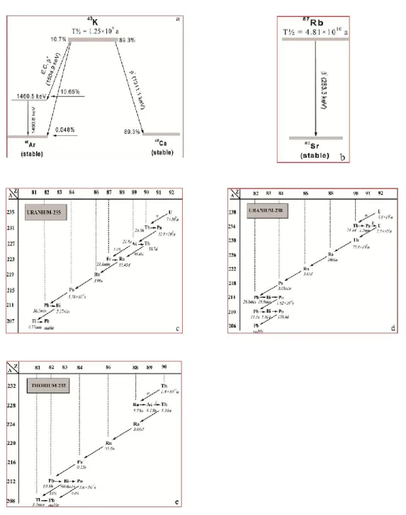
The annual radiation dose in luminescence dating originates from the ionizing radiation (α, β and γ radiations) of naturally occurring, long-lived primordial radionuclides (235U, 238U, 232Th, 40K and 87Rb) present in the sample and its immediate surroundings and from cosmic radiation.
When nuclei of 40K with a natural atomic abundance of 0.0117% undergo radioactive decay, beta particles and a gamma ray are emitted. For 87Rb, there is emission of β-particles only. The radioactive decay schemes of 40K and 87Rb are shown in Figs. 4a-4b. Natural uranium and thorium consist of three radioactive decay series headed by 235U, 238U and 232Th and ending in 207Pb, 206Pb and 208Pb, respectively (Figs. 4c-4d-4e).
25
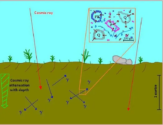
Grains are irradiated by all four types of radiation, alpha, beta, gamma and cosmic, but, because of their short range, alpha particles penetrate only the outer rind of sand-size grains (Fig. 5).
Beta particles from K and Rb are emitted within a K-feldspar grain and these deposit some of their dose within the grain before escaping. Whereas the effect of alpha particles, in minerals such as quartz and feldspars, is highly localized to within the order of 25 µm of the emitting nucleus, the upper limit to the range of the beta particles is a few millimeters (Aitken, 1985).
Considering a sphere of sediment of ~30 cm, with density of ~2 g/cm3, about 95% of the gamma radiation will be attenuate. Cosmic radiation is the most penetrating of all, attenuating by only about 14% in a meter of sediment of widespread density. In the radioactive decay chains, as shown above, each parent decays into a daughter nucleus which itself is radioactive, until the chain ends with a stable lead isotope. If the system is closed, a radioactive equilibrium or secular equilibrium is reached in which λ1N1 = λ2N2 = λiNi, where λ = (ln2)/T½ is the decay constant, N is the number of nuclei and λN is the activity. Secular equilibrium in the decay chains through time and “closed system” behaviour (i.e. physical-chemistry stability) are assumed in most luminescence dating applications, assuming that geological processes have not altered the radioactive concentrations during the entire burial period. In case of branched decay, a multiplication has to be done with the branching factor. It is important to note that, if the half-life of the parent radionuclide is much longer than that of the daughter, the latter determines the time after which equilibrium is reached. Indeed, beyond about 10 half-lives of the daughter radionuclide it decays at the same rate as it is produced - a state called secular equilibrium.
26
Fig. 4 - a, b) Decay schemes of 40K and 87Rb. c) Decay scheme for the 235U; d) 238U; e) 232Th. Data are from Lorenz (1983). A long arrow indicates alpha decay and a short one beta decay. Branching is shown except when the branching involved is less than 1%. Linking the start and end of the chains there are several radioactive daughters of 235U, 238U and 232Th that are significant since they emit a variety of α, β and γ radiations. E.g. when the nucleus
of 235U undergoes radioactive decay, with emission of an α particle, the daughter nucleus formed, 231Th, is also
27
A relevant example is the mother-daughter pair 226Ra (T½ = 1600 a) which decays to 222Rn (3.83 days), for which equilibrium is thus reached after about one month.
Fig. 5 - Schematic representation of some relevant aspects of natural radioactivity (Aitken, 1998).
METHODOLOGY
At first the sample of any geological context is drawn, and then is prudent to be certain that the sample has a relationship to the stratigraphic and/or geomorphology of the site. In Fig. 6 is possible to see the overall scheme of practical steps and procedures used for obtaining an OSL date.
28
Fig. 6 - General scheme of practical steps.
2.5 SAMPLING COLLECTION
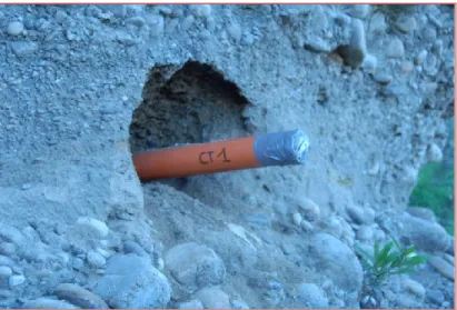
It is of critical importance that the grains of the sample are not exposed to daylight; a few seconds of this is liable to reduce the dating signal very substantially, and hence also the final age. One approach is to collect at night, first of all scraping off the surface layer and then putting the sediment in an opaque black plastic bag for transportation.
A more generally applicable approach is to push, or hammer, a steel or opaque PVC cylinder into a vertical section of the sediment. A convenient size of cylinder with a diameter of 10 cm and length of 60 cm (see Fig. 7).
29
Fig. 7 - Particular of PVC cylinder into a vertical section of the sediment.
Immediately after coring, the sampling tubes are sealed at both ends and stored so as to avoid any accidental light exposure and possible mixing of collected materials.
2.6 SAMPLE PREPARATION FOR OSL MEASUREMENTS
Under controlled lighting to avoid any natural luminescence signal loss, aliquots of coarse grained fraction are obtained following protocol after described.
In the laboratory, the outer few centimeters should be discarded as far as paleodose evaluation is concerned, even if this material can be retained for radioactivity measurements and also for the water content determination.
After drying and sieving (see Fig. 8), the sample is treated with hydrochloric acid (10% HCl) to dissolve carbonates and then hydrogen peroxide (35% H2O2) to remove organic material.
30
Fig. 8 - Example of particular step of sample preparation.
To separate the quartz fraction from both heavy minerals (>2.70 g/cm3) and feldspars (<2.62 g/cm3), solutions of sodium polytungstate of variable density are used (Mejdahl, 1985). In order to remove the outer α-irradiated layer (Aitken, 1985, 1998) and dissolve the remaining feldspars as inclusions in the quartz (Reimann et al., 2010), separated fractions are etched with hydrofluoric acid (40% HF). Finally, to eliminate any fluorides eventually produced is used hydrochloric acid (10% HCl). Considering the different penetrating powers of radiations involved (see section 2.4), the α-ray contribution from radioactivity external to the grains is eliminated as just indicated, and dose rate equation for coarse-grain dating becomes:
Dose rate = f Dβ + Dγ + Dcosm (eqn. 1.6)
The energy derived from the β rays is attenuated by the factor , related to the attenuation of β rays in dependency of grain size (Aitken, 1985).
31
The luminescence measurements are performed on small aliquots of diameter equal to 9.7 mm (Duller, 2008), composed of quartz grains within the selected size range, deposited in a monolayer onto stainless-steel discs, coated with silicon oil; in alternatively the single grains quartz are mounted on discs drilled with a 10×10 array (300 μm wide and 300 μm deep).
2.7QUARTZ AS DOSIMETERS
Various are the reasons because the OSL signals by quartz, instead of feldspars, are considered in this thesis.
The use of feldspars implicates the presence of internal 40K and some malign properties, e.g. the “anomalous fading”. This is referred to the loss of electrons from traps that are thermally stable at room temperature over geological time that could cause underestimated age. No evidence has been found to indicate that quartz OSL suffers from anomalous fading, and quartz signals are bleached more readily in daylight than feldspars OSL signals (Godfrey-Smith et al., 1988).
For these explanations it is usually necessary to separate quartz and feldspars OSL signals to obtain useful quartz dose estimates.
Moreover, it is essential to ensure the absence of the feldspars, because they could involve a change of the shape of the curve decay OSL, and finally on the OSL age value. The purity of the quartz is tested (see Table 1; Henshilwood et al., 2002
and Duller, 2003) by monitoring the presence of feldspar through measuring the IRSL signals at RT and using the approach of the (Lpost-IR OSL/T2)/(LOSL/T1) (denoted here as post-IR OSL/OSL). This test assumes that an IRSL signal at RT is emitted by feldspars. Thus, the ratio is at unity if no feldspar component is present (see Fig. 9) and it is < 1 in the case of contamination.
32
Table 1 - Feldspar contamination test (Henshilwood et al.,2002; Duller, 2003).
Step Treatment Observed
1 Give dose, Di -
2 Preheat@160-300°C for 10 s - 3 Stimulate with blue LEDS@125 °C for 40
s
LOSL
4 Give test dose, Dt -
5 Cut-heat < TPH in step 2 -
6 Stimulate with blue LEDS@125 °C for 40
s
T1
7 Give dose, Dt -
8 Preheat@160-300°C for 10 s - 9 Stimulate with IR LEDS@50 °C for 100
s
- 10 Stimulate with blue LEDS@125 °C for 40
s
Lpost-IR OSL
11 Give test dose, Dt -
12 Cut-heat < TPH in step 2 -
13 Stimulate with blue LEDS@125 °C for 40
s
T2
For the natural sample, I = 0 and D0 = 0 Gy.
Li and Ti are derived from the initial OSL signal minus a
background estimated from the last part of the stimulation curve.
Fig. 9 - Results from feldspar contamination test. The OSL and post-IR OSL curves overlap, because etching treatment (40% HF for 10 min) has removed the feldspar content.
2.8 OSL MEASUREMENTS
All luminescence measurements are made using a semi-automated Risø reader TL-DA-15 (for instrumental parameters see Appendix A) carried out by PH3DRA (Physics for Dating Diagnostic Dosimetry Research and Applications) laboratory, at Department of Physics and Astronomy of Catania (Italy).
The modified single-aliquot regenerative-dose (SAR) protocol (for details see following section) of Murray and Wintle (2000, 2003) proposed to determinate the equivalent dose (De) of coarse grained quartz, incorporates several test that attempt
to simulate natural bleaching and to check on the luminescence behaviour of the minerals and hence the suitability of the measurement procedure. The natural OSL
33
signal is measured and in the process light-sensitive traps are emptied of trapped charge. A laboratory dose Di is then given to the sample and a regenerated OSL
signal measured. This procedure can be repeated any number of times and by varying the regeneration doses, a dose response curve (also known as a growth curve) showing how the OSL signal grows with radiation dose can be constructed. Interpolating the natural OSL signal onto this growth curve gives the laboratory dose (the equivalent dose) required to induce an OSL signal equivalent to the natural OSL signal.
However, dose estimation is complicated by the fact that the sample needs to be preheated prior to OSL measurement. Franklin et al. (1995) concluded that the quartz TL peaks located at 110°, 180°, 220° and 325 °C all use the same luminescence centre, which is accessed via the conduction band. Thus, in order to be able to compare natural and regenerated signals the unstable contributions to the observed OSL signal (probably originating from the 110°, 180° and 220 °C TL traps) must be removed. One way of doing this is by preheating the sample, i.e. to heat the sample prior to OSL measurement. Unfortunately, the major luminescence sensitivity change usually seems to occur when the sample is first heated. The first true SAR protocol able to overcome the problem of sensitivity changes in quartz was described by Murray and Roberts (1998) and improved by Murray and Wintle (2000). In the SAR protocol sensitivity changes are explicitly monitored and corrected by the insertion of a test dose. All OSL measurements are carried out at 125 °C in order to prevent re-trapping of charges from the shallow trap corresponding to the 110 °C TL peak (Murray and Wintle, 1998).
There are many published descriptions of the SAR protocol and its applications (e.g. Murray and Olley, 1999; Bailey et al., 1997; Stokes et al., 2001). In the
34
following a brief description of the modified SAR (Murray and Wintle, 2003) protocol is presented and a generalised measurement sequence is shown in Table 2.
Table 2 - Experimental parameters of modified SAR protocol used for De determination (after Murray and
Wintle 2003).
a L
i and Ti are derived from the initial OSL signal minus a background estimated from the last part of the stimulation
curve.
b R is recuperation (to minimize the thermal transfer of charges possible; Choi et al., 2003; Murray and Wintle, 2003; Wintle and Murray, 2006).
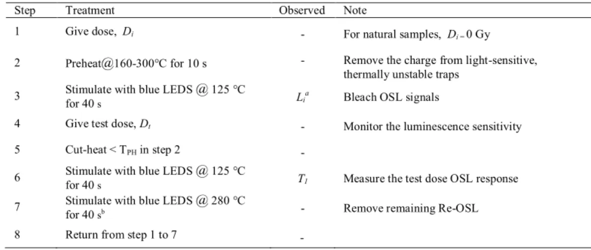
2.8.1SINGLE-ALIQUOT REGENERATIVE-DOSE (SAR) PROTOCOL
Since the last event of bleaching, to mineral is given a dose Dn before sampling.
In the laboratory the sample is, at first, preheated to a temperature TPH (usually between 160° and 300°C and held for 10 s). The natural OSL signal Ln is then measured by optical stimulation until the signal has decayed to a negligible level (i.e. until the OSL traps are empty). A small test dose Dt (usually ~10% of the
natural dose Dn) is then administered to the sample. The sample is subsequently
heated to a temperature TCH (typically 160°C to empty the 110°C TL trap), cooled immediately and the OSL signal Tn induced by the test dose measured. The second measurement cycle in the SAR protocol is initiated by giving the first regenerative dose D1 to the sample. After irradiation the sample is heated to the same preheat
Step Treatment Observed Note
1 Give dose, Di - For natural samples, Di = 0 Gy
2 Preheat@160-300°C for 10 s - Remove the charge from light-sensitive, thermally unstable traps
3 Stimulate with blue LEDS for 40 @ 125 °C
s Li
a Bleach OSL signals
4 Give test dose, Dt - Monitor the luminescence sensitivity
5 Cut-heat < TPH in step 2 -
6 Stimulate with blue LEDS for 40 @ 125 °C
s T1 Measure the test dose OSL response
7 Stimulate with blue LEDS @ 280 °C
for 40 sb - Remove remaining Re-OSL
35
temperature TPH as in the first measurement cycle and the regenerated signal L1 measured. The sample is then given another test dose Dt (same as in the first cycle),
heated to TCH and the induced OSL signal T1 measured.
In order to build a growth curve the second regenerative cycle is repeated, but increasing the size of the regenerative dose Di (see Fig. 10).
It is the OSL response to the fixed test dose Dt that is used to monitor sensitivity
changes occurring in the measurement protocol. If no sensitivity changes took place all values of Ti would be identical. By dividing the natural and regenerated OSL signals with the subsequent test dose signals (i.e. Ln = Tn and Li = Ti respectively) a sensitivity-corrected measure of the OSL signal is obtained. The regeneration doses are typically chosen such that the sensitivity corrected values Ri = (Li/Ti) encompass the natural sensitivity corrected value Rn = (Ln/Tn), i.e. 1) R1 < Rn; 2) R2 ~Rn and 3) R3 > Rn. A sensitivity-corrected growth curve is constructed by plotting values of R as a function of D. The natural dose Dn is then estimated by interpolation of the
ratio Rn onto the sensitivity corrected growth curve (see Fig. 11).
Fig. 10 - Graphical presentation of regenerative curves together to natural OSL signal.
Fig. 11 - The equivalent dose (De) is obtained by
projection of the sensitivity-corrected natural value onto the sensitivity-corrected dose response curve.
36
If the correction for sensitivity change works properly the corrected OSL ratio Ri should remain constant throughout the measurement cycle for a fixed Di, i.e. it
should be independent of prior dose and thermal treatment. This is tested in the SAR protocol by repeating one of the regeneration cycles, usually the 6th cycle is a repetition of the 2nd cycle, i.e. D5 = D1.
The ratio R5 = R1 is called the recycling ratio and if the protocol corrects for sensitivity change, should ideally be equal to unity, then R5 = R1 = 1.
If no dose (D = 0 Gy) is administered to a sample, no detectable OSL signal should be observed. In practice, however, a detectable recuperated OSL signal is seen (Aitken and Smith, 1988). In the SAR protocol the recuperation is estimated by inserting a measurement cycle with Di = 0 Gy (usually i = 4). The ratio R4 should ideally be zero, but is in practice finite. One of the prime reasons for preheating is to prevent contamination of the regenerated signals by contributions from thermally unstable but light-sensitive traps. However, preheating can also result in recuperation of the OSL signal after the OSL traps have been emptied optically.
Murray and Wintle (2000) suggested that the recuperated signal (at least in part) arises from charge inserted by the test dose into thermally shallow but light-insensitive traps, which are not emptied by heating to TCH (usually 160°C), but are emptied by heating to TPH (usually 280°C) and partly re-trapped by the OSL trap. In fact at the end of each run the aliquots or single grains are optically stimulated at 280°C for 40 s to bleach the remaining OSL signal as much as possible to minimize the thermal transfer of charges (Choi et al., 2003; Murray and Wintle, 2003; Wintle and Murray, 2006) and to prevent signal carry over to the next cycle. This value should not exceed 5% of the sensitivity corrected natural signal Murray and Wintle (2000). In general, the growth curve will often appear linear at low dose levels, but at higher dose levels the luminescence signal saturates, because of a finite number
37
of available charge traps. The growth curve is usually fitted adequately by a single saturating exponential (Thomsen, 2004).
2.8.2REJECTION CRITERIA
In order to check whether the first sensitivity measurement (Tn) is appropriate to the natural signal (Ln), to assess the reliability of De interpolation in the SAR
protocol and to confirm that pre-heating has not induced a significant difference in luminescence sensitivity between the natural and regenerated measurements, it is suggested a test, called dose recovery (Roberts et al,. 1999; Murray and Wintle, 2003). This is carried out on unheated portions that have given a laboratory dose, approximately equal to their De estimates, following removal of naturally trapped
charge by optical stimulation. The aim of these studies is to simulate the OSL signal using the same process as in nature. Since a known dose is given, the ability of the chosen SAR protocol to measure this dose accurately is tested directly.
The ratio of the measured dose to the known dose is calculated, and if the SAR protocol is working correctly, then this ratio will be unity. The dose recovery test also provides information on the maximum precision that can be achieved in the absence of natural variations in dose rate resulting from inhomogeneity of the bulk sample and variations in the degree of bleaching from grain to grain.
2.9 DISCUSSION OF DATING RESULTS: ANALYSIS OF DE DISTRIBUTION AND
STATISTICAL MODELS
For the aliquots/grains that passed the stringent rejection criteria (e.g. recycling ratios within 10% of unity and low recuperation), the obtained De values are plotted,
at first, as standard frequency distribution, also called histogram, getting an un-weighted mean De values. These distributions are classified, principally, in two
38
types and their characteristic shapes are related to the degree of bleaching during transport of mineral grains, following Arnold et al. (2007). Distribution type 1 is an example of an well-bleached sample, with a near-normal distribution (Fig. 12), whereas type 2 is positively skewed and has a characteristic tail of larger equivalent doses, representing a classic partially-bleached distribution (Fig. 13).
However, these diagrams do not take into account errors of the equivalent doses, the maximum of the histogram may therefore not coincide with the “true” geological dose, unless the errors are more or less uniform. Distortions of the shape of a histogram can occur by bright, but poorly bleached grains. Despite disadvantages, histograms offer easy visual information on how far a population of grains is bleached. This diagrams establishes, thus, a useful tool for visual inspection of data, but does not permit an quantitative statistical dose assessment (Goedicke, 2003).
Fig. 12 - Distribution type 1: example of an well-bleached sample. Frequency distribution (histogram) of the equivalent doses obtained from 112 single grains of sand-sized quartz.
Fig. 13 - Distribution type 2: example of a classic partially-bleached distribution. Frequency distribution (histogram) of the equivalent doses obtained from 150 single grains of sand-sized quartz.
39
To circumvent the doubts inherent in histograms, Galbraith et al. (1988, 1999)
promoted the radial plot (see Fig. 14) for the presentation of single-aliquot and single-grain data. The radial plot displays not only the De value for an aliquot/grain
(found by drawing a line from the y-axis (“standardized estimate”) origin through the dose point of interest until it intersects the radial axis, at the value of the equivalent dose, on the right-hand side), but also its measurement uncertainty (expressed as the standard error, found by extending a line vertically to intersect the x-axis). The latter is displayed as both “relative error” and as its reciprocal (“precision”), so that the dose estimates measured with the highest precision plot farthest to the right. These display both the individual De values and the related
precision on a plot that also enables visual evaluation of whether a sample is dominated by one population of De values, or is more complex.
Though not designed as an analytical tool, radial plots may serve to filter out data from a group that are placed within an area of ±2σ relative to an arbitrary central value (Galbraith et al., 1990, 1999). Assuming that the “true” geological dose is found within the low dose region of a distribution, a possible approach of finding this dose may consist in selecting data points by moving the 2σ area over the distribution so that the data with the lowest doses are included in the 2σ-band. The advantage of this evaluation over the evaluation of histograms is that errors are properly accounted for. An estimate for the equivalent dose is then calculated as the weighted mean of the data within the ±2σ band. It must be emphasized that the selection of data is based on a 2σ level, the final weighted mean, however, is quoted with a 1σ error.