Doctor–patient differences in risk and time preferences: A field
experiment
Matteo M. Galizzi
a,b,*, Marisa Miraldo
b,c, Charitini Stavropoulou
d, Marjon van der Pol
e aDepartment of Social Policy, Behavioural Research Lab, LSE Health, London School of Economics, Old 2.35 Old Building, Houghton Street, London WC2A 2AE, UKbÉcole d’Économie de Paris, Hospinnomics, Paris School of Economics, Hôtel-Dieu, 1, Parvis de Notre-Dame, Bâtiment B1, 5° étage, 75004 Paris, France cManagement Group, Imperial College Business School, South Kensington Campus, London SW7 2AZ, UK
dSchool of Health Sciences, City, University of London, Northampton Square, London EC1V 0HB, UK
eHealth Economics Research Unit, University of Aberdeen, Polwarth Building, Foresterhill, Aberdeen AB25 2ZD, UK
A R T I C L E I N F O Article history:
Received 2 May 2015
Received in revised form 4 October 2016 Accepted 7 October 2016
Available online 19 October 2016
JEL classification: D91 D03 I1 C93 Keywords: Field experiments Risk aversion Impatience Doctor–patient relationship Structural estimation A B S T R A C T
We conduct a framed field experiment among patients and doctors to test whether the two groups have similar risk and time preferences. We elicit risk and time preferences using multiple price list tests and their adaptations to the healthcare context. Risk and time preferences are compared in terms of switch-ing points in the tests and the structurally estimated behavioural parameters. We find that doctors and patients significantly differ in their time preferences: doctors discount future outcomes less heavily than patients. We find no evidence that doctors and patients systematically differ in their risk preferences in the healthcare domain.
© 2016 Elsevier B.V. All rights reserved.
1. Introduction
The doctor–patient interaction is generally modelled as an agency relationship (Iizuka, 2007; McGuire, 2000; Stavropoulou, 2012). Due to information asymmetry, the doctor acts as an agent making de-cisions on behalf of the patient. In a perfect agency model, doctors’ decisions should reflect patients’ preferences. In the case of health decisions patients’ risk preferences – the desire for taking a gamble – and time preferences – the degree to which the present is valued more than the future – are of particular interest (Bradford et al., 2014; Bradford, 2010; Cairns and Van der Pol, 1997; Dolan and Gudex, 1995; Gafni and Torrance, 1984; Gurmankin et al., 2002; van der Pol and Cairns, 2001, 2002, 2008; Van Der Pol, 2011; Van Der Pol and Cairns, 1999). The agency relationship may not be perfect as
doctors cannot easily observe or interpret patients’ preferences (Fagerlin et al., 2011; Say and Thomson, 2003; Ubel et al., 2011). If doctors make decisions on the basis of their own rather than pa-tients’ preferences, it is important to understand whether the two parties have similar preferences for risk and time.
The importance of risk and time preferences in medical decision-making has been extensively discussed in the medical literature. From screening tests (Edwards et al., 2006) and general practice (Edwards et al., 2005) to specialist visits for cardiovascular condi-tions (Waldron et al., 2010), almost every doctor–patient consultation involves a discussion of the trade-offs between risks and benefits of treatments over time before a treatment decision is made (Zikmund-Fisher et al., 2004). Evidence suggests that doctors’ risk and time preferences affect treatment decisions (Allison et al., 1998; Fiscella et al., 2000; Franks et al., 2000; Holtgrave et al., 1991); and that patients’ risk and time preferences have an impact on the uptake of vaccinations, preventive care, and medical tests (Axon et al., 2009; Bradford, 2010; Bradford et al., 2010; Chapman and Coups, 1999; Picone et al., 2004) and on treatment adherence (Brandt and Dickinson, 2013; Chapman et al., 2001). This means that if doctors and patients vary in terms of risk and time preferences and doctors
* Corresponding author. Department of Social Policy, Behavioural Research Lab, LSE Health, London School of Economics, Old 2.35 Old Building, Houghton Street, London WC2A 2AE, UK. Fax:+44 (0)20 7955 7345.
E-mail addresses:[email protected](M.M. Galizzi),[email protected] (M. Miraldo),[email protected](C. Stavropoulou),[email protected] (M. van der Pol).
http://dx.doi.org/10.1016/j.jhealeco.2016.10.001 0167-6296/© 2016 Elsevier B.V. All rights reserved.
Contents lists available atScienceDirect
Journal of Health Economics
cannot readily observe these differences, doctors may recommend treatments that are not optimal given patients’ risk and time preferences, which may result in lower treatment adherence. Treat-ment adherence is of major concern and has been shown to vary across individuals (WHO, 2003). Some of this variation may be due to differences in risk and time preferences between doctors and pa-tients. Better matching of doctors to patients may therefore improve health outcomes through better treatment allocation and adherence. Although the medical literature provides broad evidence on the key role of doctor–patient communication on healthcare deci-sions (Bjerrum et al., 2002; Dudley, 2001; Fagerlin et al., 2005a, 2005b, 2005c; Kipp et al., 2013; Ortendahl and Fries, 2006; Peele et al., 2005), there is little evidence on whether patients and their doctors have similar or different risk and time preferences. This gap in the evidence is largely due to the lack of primary data that di-rectly measure, in a quantitatively comparable way, risk and time preferences across patients and doctors.
Moreover, there is now broad evidence that risk and time pref-erences are largely domain-specific (Attema, 2012; Barseghyan et al., 2011; Blais and Weber, 2006; Bleichrodt and Johannesson, 2001; Bleichrodt et al., 1997; Butler et al., 2012; Cairns, 1994; Chapman, 1996; Chapman and Elstein, 1995; Cubitt and Read, 2007; Einav et al., 2010; Finucane et al., 2000; Galizzi et al., 2016; Hanoch et al., 2006; Hardisty and Weber, 2009; Hershey and Schoemaker, 1980; Jackson et al., 1972; MacCrimmon and Wehrung, 1990; Prosser and Wittenberg, 2007; Viscusi and Evans, 1990; Weber et al., 2002). Even within the same health domain, preferences vary across different contexts (Bradford et al., 2014; Butler et al., 2012; Harrison et al., 2005a; Szrek et al., 2012; van der Pol and Ruggeri, 2008). It is pos-sible, therefore, that doctors’ and patients’ healthcare decisions are explained not only by their risk and time preferences for mone-tary outcomes, but also (and perhaps more closely) by risk and time preferences for healthcare outcomes. No secondary data, however, currently exist that directly elicit health-related risk and time pref-erences for patients and doctors (Bradford, 2010).
In this article we attempt to fill this gap by explicitly investi-gating whether patients and their matched doctors in natural clinical settings have similar risk and time preferences for healthcare out-comes. As a robustness check, we also measure risk and time preferences in a closely comparable financial context. To the best of our knowledge, ours is the first attempt to systematically look at differences and similarities of risk and time preferences across doctors and patients in a real healthcare setting.
We conduct a ‘framed field experiment’ based onHarrison and List (2004)(an ‘extra-lab’ experiment according toCharness et al., 2013b). Field experiments are increasingly employed in exploring pref-erences (Andersen et al., 2008a, 2008b, 2014; Charness et al., 2013a; Harrison et al., 2007; Sutter et al., 2011), and in comparing them across different groups of subjects (Croson and Gneezy, 2009; Harrison et al., 2009; Masclet et al., 2009). In our field experiment we measure pa-tients’ and doctors’ risk and time preferences by adapting the multiple price list (MPL) tests proposed byHolt and Laury (2002)andTanaka et al. (2010), respectively, to the healthcare context (Galizzi et al., 2016). In order to address any issue that can potentially arise from framing and domain-specificity in preference elicitation, we also measure pa-tients’ and doctors’ risk and time preferences using the same MPL tests but in a closely comparable financial context.
We have three main results. First, there is a significant differ-ence in time preferdiffer-ences between patients and their matched doctors, with doctors discounting future health gains and financial out-comes less heavily than patients. Second, we find no systematic difference in risk preferences in the healthcare domain between pa-tients and doctors: in our sample both papa-tients and their matched doctors are mildly, but significantly, risk averse. Third, doctors and patients have significantly different risk preferences in the finance domain: whilst doctors are risk averse, patients are risk neutral.
The rest of the article is organised as follows.Section 2 con-tains a brief description of the methods whilstSection 3reports the main results.Section 4discusses the main findings in the context of the literature, whilst the last section briefly concludes.
2. Methods
2.1. Study design
We conducted a field experiment among patients and doctors in a university hospital in Athens (Laiko Hospital), Greece, in four waves between September 2010 and November 2011.1Patients were
asked to complete a questionnaire (Online Appendix A1) whilst they were waiting in the outpatients’ clinics to see their doctors. The ques-tionnaire was completed in the presence of a research assistant who explained the questions and was available for assistance during the completion of the questionnaire. The patients’ doctors were also invited to take part in the study by completing a similar question-naire. The outpatient clinics were pathology, cardiology, gynaecology, haematology, surgery, endocrinology, orthopaedics, urology, gas-troenterology, nephrology, rheumatology, ophthalmology, and otolaryngology. Patients who attend the outpatient clinics are seen by the first available doctor. They are therefore randomly assigned to their doctors. We obtained questionnaire data for 300 patients and 67 doctors. Not all patients could be matched to the doctor they saw for two reasons. First, patients did not know beforehand which doctor they would see, and some patients refused to answer further questions when leaving the clinic. Second, some doctors did not com-plete the questionnaire. A total of 144 patients (48% of patients) could be matched to their doctors.
The study was approved by the hospital’s Research Ethics Board on 6 August 2010 (protocol number ES 462).
2.2. Questionnaire and variables
The questionnaire included a number of socio-demographic ques-tions, such as the respondents’ age (Age), gender (Female), marital status (Married), education level (Educ), perception of their current financial situation (FinConstr), and whether they have children or not (Children). Patients were also asked about their health status, both by reporting their self-assessed health (SAH) and whether or not they had a chronic condition (Chronic). A full description of the variables in the questionnaire can be found in Appendix A.
2.2.1. Risk preferences
Risk preferences were measured using an adaptation of theHolt and Laury (2002)MPL test to the healthcare context (Galizzi et al., 2016). The MPL method is one of the most widely used incentive-compatible tests in experimental economics to measure risk preferences for monetary outcomes (Charness et al., 2013a). Sub-jects are presented with a series of choices between two lotteries (A and B). The payoffs in the lotteries remain constant but the prob-ability associated with each payoff changes. Lottery A is associated with a higher expected pay-off in the first few choices but this switches to lottery B in the later choices.
The MPL was adapted by presenting the lotteries as different healthcare treatments with payoffs defined as days of full health (Table 1). A risk-neutral individual should switch from the ‘safe’
1 Round 1 of data collection started in September 2010, lasted 5 weeks and in-cluded 91 patients. Round 2 started in January 2011, lasted 4 weeks and inin-cluded 34 patients. Round 3 started in April 2011, lasted 5 weeks and included 56 pa-tients. Round 4 started in October 2011, lasted 4 weeks and included 119 papa-tients. It should be noted that the survey was conducted at a time of great economic crisis. The potential implications are discussed in detail inGalizzi et al. (2016).
option (treatment A) to the ‘risky’ option (treatment B) only when the expected utility is greater in treatment B than in A. An indi-vidual who is risk neutral chooses treatment A in rows 1–4, before switching to B in row 5. A risk averse individual switches to treat-ment B after row 5, whilst a risk lover switches before row 5. Thus, the switching point is a measure of an individual’s risk prefer-ences. We define SwitchRiskHP (SwitchRiskHD) a variable denoting the point at which a given patient (doctor) switched from lottery A to lottery B. This ranges from 1 (switching to treatment B in the first row) to 10 (never switching to treatment B) and the higher the value, the more risk averse the patient (doctor) is.
2.2.2. Time preferences
Time preferences were measured using an adaptation of the
Tanaka et al. (2010)MPL to the healthcare context. Subjects were presented with a series of six blocks of choices, each of which had five choices between two different healthcare treatments. Sub-jects were asked to consider their current health status and to choose between two possible hypothetical treatments, A and B, with dif-ferent days of full health at difdif-ferent points in time (Table 2). In each block, treatment A gave a larger number of days in full health than
treatment B. Treatment A, however, was offered with some delay (so-called Larger-Later option, LL) whilst treatment B was always available immediately (so-called Smaller-Sooner option, SS). Treat-ment B offered progressively a larger number of days in full health. The time delay varied between blocks of lotteries from 1 week (blocks 1 and 4) to 1 month (blocks 2 and 5), to 3 months (blocks 3 and 6). We used switching points as simple measures of individ-ual time preferences. The later individindivid-uals switch from treatment A to treatment B the more patient they are. The variable
SwitchTimeHPBi (SwitchTimeHDBi) denotes the specific point at which
a given patient (doctor) switched from option A to option B in the block of questions i. The values range from 1 to 6 and the higher the value, the more patient the subject is.
2.3. Analysis
We examine differences in risk and time preferences between patients and doctors using two measures for individual prefer-ences. First, we examine switching points in the MPL tests as indicators of individual risk and time preferences. The higher the value of the SwitchRiskHP (SwitchRiskHD) variable, the more risk
Table 1
Adaptation of theHolt and Laury (2002)MPL test to measure risk preferences in the healthcare domain.
ID Treatment A Treatment B Your Choice
P Days in full health P Days in full health P Days in full health P Days in full health A B
1 10% 200 90% 160 10% 385 90% 10 A B 2 20% 200 80% 160 20% 385 80% 10 A B 3 30% 200 70% 160 30% 385 70% 10 A B 4 40% 200 60% 160 40% 385 60% 10 A B 5 50% 200 50% 160 50% 385 50% 10 A B 6 60% 200 40% 160 60% 385 40% 10 A B 7 70% 200 30% 160 70% 385 30% 10 A B 8 80% 200 20% 160 80% 385 20% 10 A B 9 90% 200 10% 160 90% 385 10% 10 A B Table 2
Adaptation of theTanaka et al. (2010)test to measure time preferences in the healthcare domain.
ID Treatment A Treatment B Your choice
1.1 360 days in full health starting in 1 week 60 days in full health starting today A B 1.2 360 days in full health starting in 1 week 120 days in full health starting today A B 1.3 360 days in full health starting in 1 week 180 days in full health starting today A B 1.4 360 days in full health starting in 1 week 240 days in full health starting today A B 1.5 360 days in full health starting in 1 week 300 days in full health starting today A B 2.1 360 days in full health starting in 1 month 60 days in full health starting today A B 2.2 360 days in full health starting in 1 month 120 days in full health starting today A B 2.3 360 days in full health starting in 1 month 180 days in full health starting today A B 2.4 360 days in full health starting in 1 month 240 days in full health starting today A B 2.5 360 days in full health starting in 1 month 300 days in full health starting today A B 3.1 360 days in full health starting in 3 months 60 days in full health starting today A B 3.2 360 days in full health starting in 3 months 120 days in full health starting today A B 3.3 360 days in full health starting in 3 months 180 days in full health starting today A B 3.4 360 days in full health starting in 3 months 240 days in full health starting today A B 3.5 360 days in full health starting in 3 months 300 days in full health starting today A B 4.1 900 days in full health starting in 1 week 150 days in full health starting today A B 4.2 900 days in full health starting in 1 week 300 days in full health starting today A B 4.3 900 days in full health starting in 1 week 450 days in full health starting today A B 4.4 900 days in full health starting in 1 week 600 days in full health starting today A B 4.5 900 days in full health starting in 1 week 750 days in full health starting today A B 5.1 900 days in full health starting in 1 month 150 days in full health starting today A B 5.2 900 days in full health starting in 1 month 300 days in full health starting today A B 5.3 900 days in full health starting in 1 month 450 days in full starting health today A B 5.4 900 days in full health starting in 1 month 600 days in full health starting today A B 5.5 900 days in full health starting in 1 month 750 days in full health starting today A B 6.1 900 days in full health starting in 3 months 150 days in full health starting today A B 6.2 900 days in full health starting in 3 months 300 days in full health starting today A B 6.3 900 days in full health starting in 3 months 450 days in full health starting today A B 6.4 900 days in full health starting in 3 months 600 days in full health starting today A B 6.5 900 days in full health starting in 3 months 750 days in full health starting today A B
averse in healthcare a patient (doctor) is. Similarly, the higher the value of the SwitchTimeHPBi (SwitchTimeHDBi) variable the more patient in healthcare a patient (doctor) is. The Shapiro–Wilk test for normality rejects the null hypothesis that the switching points are normally distributed and we therefore test for differences in means between patients and doctors using the non-parametric (Wilcoxon) Mann–Whitney test. Even though doctors and pa-tients may on average differ in their time and risk preferences, it could be the case that there is no difference in preferences in matched doctor–patient pairs and vice versa. It is therefore impor-tant to examine the difference in matched pairs as well as the difference in overall mean between doctors and patients. This is done by examining the number of patients who have identical or similar switching points to their doctors. We test for differences in switch-ing points in matched pairs usswitch-ing the Wilcoxon matched-pairs signed-ranks test. As mentioned previously, 48% of patients can be matched to their doctor. Statistical tests (chi-square and t-tests) show that this sub-sample is similar to the whole sample in terms of socio-demographic characteristics.
Second, we ‘structurally’ estimate the behavioural parameters within the utility functions. We separately estimate risk and time preferences following the empirical approaches byHarrison and Rutström (2008a), Andersen et al. (2010), andTanaka et al. (2010). We assume that the health-related risk preferences can be repre-sented by a constant relative risk aversion (CRRA) utility function. The utility function of a subject in terms of healthcare payoffs x, is thus represented by U x x s s
( )
= − − 1 1 (1)where s is the coefficient of constant relative risk aversion in the healthcare context. Depending on the value of s a subject shows dif-ferent degrees of risk aversion in the healthcare domain that can be grouped in three main types:
1. if s= 0 risk neutral
2. if s> 0 risk averse
3. if s< 0 risk seeking
Maximum Likelihood (ML) methods were used to empirically es-timate risk preferences (Harrison and Rutström, 2008aandAndersen et al., 2010). From Equation(1)U(x) is the utility that a subject
per-ceives from getting a healthcare benefit x. Under Expected Utility Theory, the expected utility by a subject of a given lottery j= A,B is
the utility of each outcome k= 1,2 in that lottery, weighted by the probability pkof the outcome:
EUj=
∑
k=1 2, pkj∗U x( )
kj (2)with j= A,B and k = 1,2. The expected utility depends on the
sub-ject’s risk aversion parameter s. Based on a candidate value of s a latent preference index Δ(EU) can be constructed. Our empirical model allows subjects in the outpatient clinics to make stochastic errors when comparing expected utilities. We include in our esti-mation a parameter μ to capture the stochastic error, so that the latent index is:
Δ EU EU EU EU A A B
( )
=(
)
(
)
+(
)
1 1 1 μ μ μ (3)When μ→0 the stochastic errors become negligible and the
em-pirical specification reduces to a deterministic EUT choice, where the subject always chooses the lottery with higher perceived ex-pected utility. When, however, μ gets larger, μ→ ± ∞, the choice
between the two lotteries becomes essentially random, with the
value of the latent index function approaching 1/2 for any values of the expected utilities. We assume that the latent index Δ(EU) follows a logistic cumulative density function (CDF) taking values between 0 and 1, so that Λ(Δ(EU)) can be thought to link the latent preferences and the binary choices observed in the experiment (1):
Prob choosing lottery A
(
)
=Λ Δ
(
( )
EU)
(4)Under the assumptions of Expected Utility Theory and of CRRA utility functions, the likelihood of observing a specific choice depends on the individual risk preference s, given the logistic CDF linking the latent index to the observed choices. The individual log-likelihood of choosing either lottery in each of the observed choices
Ci, in our experiment is given by:
Ln L s
(
, ;μ
C)
=∑
i(
(
lnΛ Δ
(
( )
EU)
Ci=1)
+(
(
lnΛ
(
1−Δ
( )
EU)
Ci=0)
(5)where Ci=1(0) denotes the choice of lottery A(B) in the proposed
pair of lotteries i. The ML was adjusted to allow the CRRA param-eter s to be a linear function s= s0+ s1D where D is a dummy variable
taking value 1 for doctors and 0 for patients.
For time preferences we follow the procedure byTanaka et al. (2010)to estimate the shape of the discounting function for pa-tients and doctors.Tanaka et al. (2010)use a general discounting model originally proposed byBenhabib et al. (2010)which allows to test exponential, hyperbolic, and quasi-hyperbolic discounting as ‘nested’ cases of a more general discounting function. The dis-counting model assigns to a healthcare benefit y at time t> 0 a value of
y
β
(
1− −(
1θ
)
rt)
1 1( )−θ (6)(and a value y for immediate healthcare benefit at t= 0). The three factors r, β, and θ identify the levels of baseline time discounting (r), present bias (β), and hyperbolicity of the discounting function (θ), respectively.
This general discounting model nests the three most common discounting specifications as special cases. In particular, when β= 1 as θ→ 1 the discounted value reduces to the conventional expo-nential discounting model in the limit,e−rt(Samuelson, 1947). When
β= 1 as θ = 2 the discounted value reduced to the ‘pure hyperbol-ic’ discounting model, 1
1+ ⎛
⎝⎜ rt⎞⎠⎟ (Loewenstein and Prelec, 1992). 2
When, finally, θ→ 1 and β is a free parameter, then the discounted value reduces to the ‘quasi-hyperbolic’ or ‘present bias’ discount-ing model βe−rt (Laibson, 1997; Phelps and Pollak, 1968).
We denote the probability of choosing immediate reward of x over the delayed reward of y in t days by P x
(
>( )
y t,)
and use a lo-gistic function to describe this relationship (7):P x y t x y rt >
( )
(
)
= +(
−(
−(
− −(
)
)
−)
)
, exp 1 1μ
β
1 1θ
1 1θ (7)where r,β,θ are the above defined parameters, and μ is a response sensitivity or ‘noise’ parameter.
2 The ‘hyperbolic’ model originally proposed byLoewenstein and Prelec (1992) actually takes the more general form where the parameter h can be interpreted as a measure of ‘decreasing impatience’ (Attema et al., 2010; Bleichrodt et al., 2014; Prelec, 2004; Rohde, 2010). When h= 0, the hyperbolic discounting is equivalent to exponential discounting. The higher the h, the more individual discounting devi-ates from constant discounting. TheLoewenstein and Prelec (1992)general hyperbolic model nests further specific models such as the ‘power’ discounting model when h= 1 (Harvey, 1986, 1995), and the ‘proportional’ discounting model when h= r (Mazur, 1987), which is the ‘pure hyperbolic’ specification fitted in our estimations.
A dummy variable for doctors is included in the models to examine whether parameters vary across doctors and patients. For example, for the ‘present bias’ model, we fit a logistic function (8)
P x y t x y ert >
( )
(
)
= +(
−(
− −)
)
, exp 1 1μ
β
(8)where β= β0+ β1D, r= r0+ r1D, and D is a dummy variable taking value 1 for doctors and 0 for patients.
All estimates were obtained using an iterative nonlinear least square regression procedure with standard errors clustered at in-dividual level, and a minimum number of 100 iterations at 99 percent significance level. When initial values had to be specified in order to help convergence of estimations, multiple replications were per-formed using a range of different initial values.
2.3.1. Robustness checks and further analysis
Both the time and risk preference tasks were conducted from the perspective of the subject’s current health status. This raises two issues. First, the size of the health gain from the treatment varies across subjects depending on the level of their current health. The health gain is likely to be larger on average for patients compared to their doctors. Earlier empirical evidence suggests that individu-als tend to be more risk averse for larger gains although this is now being debated (Harrison et al., 2005b; Holt and Laury, 2002, 2005). If true, this may bias the results towards patients being more risk averse. The time preference literature suggests that individuals dis-count larger gains at a lower rate than smaller gains (Andersen et al., 2013; Benzion et al., 1989; Chapman and Elstein, 1995; Green et al., 1997; Kirby and MarakoviC´, 1996; Scholten and Read, 2010; Thaler, 1981). This may bias the results towards patients being more patient. To explore this we examine whether switching points are a func-tion of self-assessed health using both a chi-square test and a Pearson correlation coefficient. The estimated difference between doctors and patients is less likely to be biased by differences in health gains if there is no statistically significant relationship between self-assessed health and switching point. If there is a significant relationship the sign of the correlation will indicate the direction in which the results may be biased.
Secondly, the use of current health state raises the issue of sa-tiation in subjects who are in full health. Individuals may express indifference (zero time preference and risk neutrality) in that case or not engage with the tasks. We explore this by replicating the anal-ysis excluding subjects who reported to be in full health.
To further test the robustness of our results, we also compare time and risk preferences between patients and doctors in the finance domain using theTanaka et al. (2010)MPL test and theHolt and Laury (2002)MPL test (Online Appendix A2). In the financial domain, the size of the gain is the same across all subjects and none of the subjects will be satiated. Whilst time and risk preferences have been shown to be domain specific (Attema, 2012; Barseghyan et al., 2011; Blais and Weber, 2006; Bleichrodt and Johannesson, 2001; Bleichrodt et al., 1997; Butler et al., 2012; Cairns, 1994; Chapman, 1996; Chapman and Elstein, 1995; Cubitt and Read, 2007; Einav et al., 2010; Finucane et al., 2000; Galizzi et al., 2016; Hanoch et al., 2006; Hardisty and Weber, 2009; Hershey and Schoemaker, 1980; Jackson et al., 1972; MacCrimmon and Wehrung, 1990; Prosser and Wittenberg, 2007; Viscusi and Evans, 1990; Weber et al., 2002), it could be argued that, if the domain effect is similar across pa-tients and doctors, then the difference in preferences between doctors and patients should be similar across domains. Similar differences across the two domains would increase the confidence we can place on the healthcare results.
3. Results
3.1. Summary statistics
The summary statistics for the two samples of patients and doctors are reported inTable 3. Due to missing values the sample size for estimating time and risk preferences varies from 241 to 294 for patients and from 56 to 66 for doctors. The four patients who switched back in the time preference tasks were omitted from the analysis.
The statistics show that, with the exceptions of income (and education) levels, age, and self-assessed health, doctors and pa-tients in our sample have comparable socio-demographic characteristics.
Table 3
Descriptive statistics.
Variable N Mean Std. Dev. Min Max N Mean Std. Dev. Min Max
Patients Doctors SwitchHRisk 281 5.06 2.57 0 10 58 5.03 2.05 1 10 SwitchHTimeB1 273 4.39 1.93 1 6 63 4.88 1.69 1 6 SwitchHTimeB2 265 3.35 2.03 1 6 60 4.2 1.93 1 6 SwitchHTimeB3 252 2.68 2.02 1 6 61 3.52 1.98 1 6 SwitchHTimeB4 248 4.63 1.89 1 6 60 4.8 1.91 1 6 SwitchHTimeB5 242 3.41 2.01 1 6 56 4.12 2.15 1 6 SwitchHTimeB6 241 2.81 2.03 1 6 56 3.8 2.14 1 6 SwitchFRisk 294 4.90 2.75 1 10 59 5.52 2.36 1 10 SwitchFTimeB1 294 4.12 1.98 1 6 66 4.77 1.65 1 6 SwitchFTimeB2 293 3.05 1.88 1 6 65 4.36 1.62 1 6 SwitchFTimeB3 292 2.43 1.77 1 6 66 3.64 1.77 1 6 SwitchFTimeB4 291 4.67 1.87 1 6 65 5.14 1.39 1 6 SwitchFTimeB5 290 3.71 1.97 1 6 66 4.44 1.63 1 6 SwitchFTimeB6 289 2.69 1.83 1 6 66 3.57 1.81 1 6 Age 238 39.61 12.93 18 74 61 36.59 8 27 63 Female 300 0.48 0.50 0 1 67 0.46 0.50 0 1 Educ 238 5.59 1.63 2 8 Married 300 0.34 0.47 0 1 67 0.38 0.49 0 1 Children 300 0.34 0.47 0 1 67 0.23 0.43 0 1 FinConstr 232 2.45 0.74 1 4 60 2.03 0.66 1 3 SAH 300 2.39 1.16 1 5 67 1.62 0.73 1 4 Chronic 300 0.17 0.37 0 1
3.2. Switching points measures for risk and time preferences: differences between patients and doctors
We start by examining differences in risk preferences. The mean switching point in the healthcare domain was SwitchHRiskP= 5.06 (SD= 2.57) for patients and SwitchHRiskD = 5.03 (SD = 2.05) for doctors. The Mann–Whitney test failed to reject the null hypoth-esis that SwitchHRiskP= SwitchHRiskD (z = −0.332, p = 0.7401), suggesting that health-related risk preferences are similar for doctors and patients.
The lack of significance of the chi-square test and the Pearson correlation (p= 0.433 and p = 0.0875 respectively) suggest that there
is no significant relationship between risk preferences and self-assessed health. The potential difference in the size of the health gain between doctors and patients is therefore unlikely to have biased the comparison. To further test the robustness of the results we also compare risk preferences in the financial domain. The mean switch-ing point in the finance domain was SwitchFRiskP= 4.90 (SD = 2.75) for patients, whilst for the doctors it was SwitchFRiskD= 5.52 (SD= 2.36). The Mann–Whitney rejects the null hypothesis that
SwitchFRiskP= SwitchFRiskD at a 95% significance level (z = −1.973, p= 0.0485), suggesting a significant difference in the
finance-related risk preferences between the two groups, with the doctors being more risk averse in finance than patients.
In case of time preferences, a relatively large proportion of doctors and patients never switched from option A to option B, with the exact proportion varying per block of questions. In the healthcare domain the percentage of respondents never switching were 50% in the first block, 28% in the second, 19% in the third, 57% in the fourth block, 32% in the fifth and 25% in sixth block. Similar figures hold for the finance domain.
Table 4shows that in healthcare the mean switching points for doctors are higher across all six blocks of pairwise choices, and the doctor–patient differences are significant in all cases but the fourth block. Note that the doctor–patient differences are only
marginal-ly significant in the first block. This suggests that doctors are more patient when discounting future health outcomes than patients, at least for time delays longer than a week. The significance of the chi-square test and the Pearson correlation suggest that there is a significant relationship between time preferences and self-assessed health (p-values for chi-square test range from 0.0001 to 0.1001 across the six blocks, and the p-values for the Pearson correlation range from 0.0000 to 0.0001). The correlation is negative suggest-ing that larger health gains (lower self-assessed health) are discounted at a higher rate. The difference in time preferences may therefore be caused by the difference in current health status between doctors and patients. To explore this further we also compare time preferences in the financial domain.Table 4shows that the results for time preferences for money are very similar in that doctors are significantly more patient than their patients.
Table 5shows the difference in switching points between matched doctor–patient pairs. The proportion of patients who have identi-cal time and risk preferences to their doctor ranges from 19.5% for risk preferences to 38.9% for time preferences (fourth block). Switch-ing points are 2 or more apart from their doctors for around 50% of patients. The results of the Wilcoxon matched pairs test are in line with the results for the aggregate preferences. There are no dif-ferences in risk predif-ferences but matched doctor–patients do differ in terms of their time preferences. That the results are similar is perhaps not surprising given that patients in our outpatient clinics were randomly assigned to a doctor.
3.3. Structural estimation of risk and time preferences: differences between patients and doctors
Table 6shows the ML results which allow the fitted param-eters to be a function of a doctor dummy variable, in order to estimate differences across the two types of respondents. The es-timates for the two subsamples of doctors and patients are reported in Appendix B and are in line with the pooled results. The table also
Table 4
Differences in time preferences between doctors and patients.
TimeB1 TimeB2 TimeB3 TimeB4 TimeB5 TimeB6
Healthcare
Number of patients 273 265 252 248 242 241
Number of doctors 63 60 61 60 56 56
Switching point mean patients 4.39 3.35 2.68 4.63 3.41 2.81
Switching point mean doctors 4.88 4.2 3.52 4.8 4.1 3.80
z statistic −1.911 −2.770 −2.940 −0.899 −2.249 −2.937
p-value 0.0560 0.0056 0.0033 0.3685 0.0245 0.0033
Finance
Number of patients 294 293 292 291 290 289
Number of doctors 66 65 66 65 66 66
Switching point mean patients 4.12 3.06 2.43 4.67 3.71 2.69
Switching point mean doctors 4.77 4.35 3.64 5.14 4.44 3.57
z statistic −2.343 −4.941 −4.985 −1.457 −2.555 −3.558
p-value 0.0191 0.0000 0.0000 0.1451 0.0106 0.0004
Note: P-values refer to tests of the null hypothesis that switching points are not statistically significantly different across patients and doctors.
Table 5
Difference in switching point in matched doctor–patient pairs.
No difference Difference of 1 point Difference of more than 1 point Wilcoxon matched pairs test
N % N % N % p-value SwitchHRisk 24 19.5 31 25.2 68 55.3 0.1074 SwitchHTimeB1 43 33.6 17 13.3 68 53.1 0.0002 SwitchHTimeB2 32 27.4 21 17.9 64 54.7 0.0000 SwitchHTimeB3 38 35.2 14 13.0 56 51.9 0.0000 SwitchHTimeB4 42 38.9 8 7.4 58 53.7 0.0036 SwitchHTimeB5 34 34.3 13 13.1 52 52.5 0.0125 SwitchHTimeB6 34 35.4 12 12.5 50 52.1 0.0000
shows that the doctor dummy variable is not statistically signifi-cant in the estimates for the CRRA parameter in the healthcare domain, confirming that there are no systematic differences in risk preferences for healthcare outcomes across doctors and patients. The doctor dummy variable is also not significant in the estimates for the stochastic error μ, suggesting that doctors and patients are equally likely to make errors in their responses to the test. In the finance domain, the doctors’ dummy variable is significantly asso-ciated with both the CRRA and the noise coefficient: doctors are more risk averse in finance than patients, and also make fewer errors in their choices compared to patients.
As for time preferences, due to the relatively small number of observations for the doctors, we were unable to reliably fit the general discounting model. We therefore focus on the estimation of the three ‘nested’ discounting models: (i) the ‘exponential’ model; (ii) the ‘pure’ hyperbolic discounting model; and (iii) the ‘quasi-hyperbolic’ or ‘present bias’ model.Table 7shows the results for the three differ-ent discounting models.3In the healthcare domain, the estimated
coefficient for the doctor dummy variable is negative and highly sig-nificant in both the ‘exponential’ and the ‘pure hyperbolic’ model (−0.015, with SE = 0.0036, and −0.0248 with SE = 0.0064, respective-ly), suggesting that doctors are less impatient than patients. The estimated coefficient for the doctor dummy variable is also nega-tive and highly significant in the finance domain (−0.0135, with
SE= 0.0025, in the ‘exponential’ model, and −0.0237, with SE = 0.0047,
in the ‘pure hyperbolic’ model). In the ‘present bias’ model, the doctor dummy variable is negative and highly significant for the long-run discounting rates (−0.0159, with SE = 0.0034, in the healthcare domain; and−0.0096, with SE = 0.0020, in the finance domain), but does not reach statistical significance for the present bias parameter (0.0144, with SE= 0.1126, in the healthcare domain, and 0.1033, with
SE= 0.0813, in the finance domain). Estimates also confirm that doctors
are generally less impatient than patients, and that, the present bias parameter is not significantly different from one.
The goodness of fit of the estimated discounting models is rel-atively high with the adjusted R2ranging from 0.5243 to 0.5301 in the healthcare domain, and from 0.5690 to 0.5706 in the finance domain. The goodness of fit does not vary substantially across the different specifications within the same domain.
The above estimates of the risk and time preferences param-eters and of the doctor–patient dummy are robust to the introduction in the models of further covariates, such as gender, age, financial state, and self-assessed health. Finally, similar results were found when excluding subjects who reported to be in full health suggest-ing that satiation might not have been an issue (results available upon request).
4. Discussion
Our data suggest that there is no systematic difference in risk preferences in the healthcare domain between doctors and pa-tients: both doctors and patients tend to be mildly risk averse in the healthcare domain. It could be argued that the lack of signifi-cant doctor–patient differences in risk preferences in health is not due to a genuine similarity of the underlying risk preferences, but is partly an artefact of the differences in perceived health gains with doctors closer to being ‘satiated’ in health than patients.4On average,
doctors’ self-reported health was higher than patients (1.62 com-pared to 2.39). However, we found no significant relationship between risk preferences and self-assessed health. This is in line with other studies which have questioned the earlier evidence that individuals tend to be more risk averse for larger (monetary) out-comes (Harrison et al., 2005b; Holt and Laury, 2002, 2005). If the earlier evidence holds, this would imply that doctors would be more risk averse if presented with larger health gains. Therefore, the non-significant small difference in risk aversion in healthcare between patients and doctors found in our estimations may have resulted from an underestimation of risk aversion in doctors.
The use of current health state as the reference point also raises the question as to how subjects in good health answered the ques-tions as they were ‘satiated’ in their level of health. Around half of the doctors (51.25%) reported to be in very good health. However, excluding subjects who reported to be in very good health did not change the results. Given that all subjects gave reasonable and mean-ingful answers all throughout the tests, and that the estimates of the CRRA coefficient are consistent with non-satiation (e.g.Harrison and Rutström, 2008b, p. 181), it may be the case that subjects who reported being in very good health used a reference health status worse than the self-reported health at the time they participated in the experiment. That is, subjects may have made sense of the sce-nario presented in a way more consistent with the life-time health losses they experienced or expected to experience. Therefore it is possible that their answers were implicitly anchored to a poorer health status than their reported self-assessed health.
We also compared risk preferences across doctors and patients in the financial domain as a further robustness check. In the finan-cial domain, the size of the gain was the same across all subjects and none of the subjects were satiated. However, it should be noted
3 Sample size inTable 7differs across the healthcare and the finance domains due to different missing data in the different blocks of time preferences questions. In the healthcare domain, 273 patients and 63 doctors answered the first block of ques-tions; 265 patients and 60 doctors answered the second block of quesques-tions; 252 patients and 61 doctors answered the third block of questions; 248 patients and 60 doctors answered the fourth block of questions; 242 patients and 56 doctors an-swered the fifth block of questions; and 241 patients and 56 doctors anan-swered the last block of questions. Since each block had five time preferences questions, this gives a total of 9385 responses in the healthcare domain. Similarly, in the financial domain, 294 patients and 66 doctors answered the first block of questions; 293 pa-tients and 65 doctors answered the second block of questions; 292 papa-tients and 66 doctors answered the third block of questions; 291 patients and 65 doctors an-swered the fourth block of questions; 290 patients and 66 doctors anan-swered the fifth block of questions; and 289 patients and 66 doctors answered the last block of ques-tions. This gives a total of 10,715 responses in the finance domain.
4 Note that we have opted for having the same framing across patients and doctors in order to not confound the findings with differences in the framing. An alterna-tive experiment design could consist of presenting both doctors and patients with the same baseline hypothetical health status scenario. Given the non-observable dif-ferences in health status across patients, however, it would not be possible to elicit which health status (whether their own status or the hypothetical baseline status) was more salient in patients’ choices. It is plausible to presume that the most salient would be the most severe health status, implying that a patient with a cancer di-agnosis would anchor her choices to her real health status, whereas a doctor in full health would be more likely to anchor his choices to the hypothetical baseline scenario.
Table 6
Estimated risk aversion parameters under CRRA.
Healthcare domain Finance domain
s 0.1415*** 0.1211** 0.0432 −0.0135 (0.0470) (0.0522) (0.0535) (0.0578) sd −0.0138 0.0872 0.0253 0.3352*** (0.0322) (0.1092) (0.0315) (0.1173) μ 30.8911*** 34.5442*** 52.3180*** 71.8444*** (6.6939) (8.5517) (13.4195) (20.7522) μd −14.8975 −59.5904*** (12.0268) (21.5227) Observations 3051 3051 3177 3177 Log pseudo LL −1721.87 −1719.70 −1771.23 −1756.73 Notes: * p< 0.1, ** p < 0.05, ***p < 0.01. Sample size in the healthcare domain is 3051: 9 observations for 281 patients and 58 doctors. Sample size in the financial domain is 3177: 9 observations for 294 patients and 59 doctors.
that doctors in our sample are generally on higher incomes than their patients, and income is known to be associated with risk pref-erences (Donkers et al., 2001). Doctors and patients did significantly differ in their risk preferences in the finance domain, with doctors being risk averse whilst patients are risk neutral. Moreover, the es-timated CRRA coefficient for doctors in finance is higher than their CRRA coefficient in health (Appendix B), suggesting that the dif-ferences in risk predif-ferences across doctors and patients may have been underestimated in the healthcare domain. An alternative ex-planation for the difference in risk preferences in the monetary domain is the difference in income levels.
In case of time preferences, our evidence suggests that doctors are more patient than their patients when deciding over health-care treatments with benefits at different points in time. We do not find any support for present bias either in patients’ or in doctors’ time preferences for healthcare treatments. The above results are confirmed for the financial domain. We found a significant rela-tionship between time preferences and self-assessed health with larger health gains being discounted at a higher rate. The differ-ence in time preferdiffer-ences between doctors and patients may have therefore in part been caused by differences in the size of the health gain. However, we found a similar difference in time preferences between doctors and patients across the two domains.
For the health domain, the lack of present bias is in line with other recent studies which, using different methods, also reject the quasi-hyperbolic model for time preferences in health (Bleichrodt et al., 2014), but it is in contrast with earlier evidence on quasi-hyperbolic discounting for health outcomes (Cairns and Van der Pol, 1997; van der Pol and Cairns, 2002). For the finance domain, our findings may seem unexpected given the widespread support in favour of quasi-hyperbolic discounting among behavioural econo-mists (Ainslie, 1975; Angeletos et al., 2001; DellaVigna and Malmendier, 2006; Diamond and Köszegi, 2003; Gruber and Köszegi, 2001, 2004; Kirby and Marakovic´, 1995; Kirby et al., 1999; Laibson, 1997; Loewenstein and Prelec, 1992; McClure et al., 2004; O’Donoghue and Rabin, 1999; Phelps and Pollak, 1968; Strotz, 1955; Thaler, 1981).
A number of reasons can explain the differences in findings, in-cluding the hypothetical rewards, the elicitation method, the subject pool, and the study setting. More generally, some recent experimen-tal results on time preferences over monetary outcomes suggest that the evidence on hyperbolic discounting is not unanimous. For in-stance, a number of recent studies have failed to support the hypothesis of non-constant discounting, includingAndreoni and Sprenger (2012), Laury et al. (2012), andAndersen et al. (2014). Fur-thermore, a review of the literature byAndersen et al. (2014)notices that all evidence to date on non-constant discounting with
mone-tary outcomes refers either to hypothetical surveys, or to studies with no incentive-compatible rewards, or to lab experiments with student subjects. None of the studies included in the review byAndersen et al. (2014)elicits hypothetical health- and finance-related time prefer-ences from doctors and patients in real clinical settings.
Our study adds to this evidence and, to the best of our knowl-edge, is the first study to suggest that patients and doctors in real clinical settings may not exhibit any significant present bias when making decisions on healthcare treatments over time. Given that quasi-hyperbolic discounting is associated to dynamic inconsisten-cy, it is somehow reassuring to learn that, at least when it comes to healthcare decisions in real clinical settings, not only doctors but also patients exhibit time-consistent preferences. Similarly reas-suring is the finding that there is no systematic difference in risk preferences between doctors and patients whey they make deci-sions over risky healthcare treatments. However, further evidence is needed to understand whether this is due to the specific health-care domain, the clinical setting, the hypothetical nature of the decisions, or any other specific characteristics of our field study.
5. Conclusions
Preferences for risk and time are fundamental individual char-acteristics that have been found to be associated with numerous health and healthcare behaviours, including: heavy drinking (Anderson and Mellor, 2008; Bradford et al., 2014; Szrek et al., 2012), drink and driving (Sloan et al., 2014) smoking (Barsky et al., 1995; Bradford et al., 2014; Bradford, 2010; Burks et al., 2012; Dohmen et al., 2011; Goto et al., 2009), BMI (Borghans and Golsteyn, 2006; Chabris et al., 2008; Ikeda et al., 2010; Sutter et al., 2013; Weller et al., 2008), poor nutritional quality (Galizzi and Miraldo, 2012); as well as overall self-assessed health (Van Der Pol, 2011), the uptake of vaccinations, preventive care, and medical tests (Axon et al., 2009; Bradford, 2010; Bradford et al., 2010; Chapman and Coups, 1999; Picone et al., 2004) and adherence to treatments (Brandt and Dickinson, 2013; Chapman et al., 2001).
Surprisingly little attention has been paid to differences and simi-larities of risk and time preferences between doctors and their patients. These differences can potentially have a major impact on doctor–patient communication, healthcare decision-making, and treatment adherence. To the best of our knowledge, ours is the first field experiment to examine differences in risk and time prefer-ences between doctors and patients in real clinical settings.
We have three main findings. First, there is a significant differ-ence in time preferdiffer-ences across patients and their matched doctors, with doctors discounting future less heavily than patients. Second, we find no systematic difference in risk preferences in the
health-Table 7
Estimated discounting parameters under exponential, hyperbolic, and quasi-hyperbolic discounting models.
Healthcare domain Finance domain
Exponential Hyperbolic Quasi-hyperbolic Exponential Hyperbolic Quasi-hyperbolic
μ 0.0037*** 0.0042*** 0.0035*** 0.0045*** 0.0051*** 0.0048*** (0.0002) (0.0002) (0.0002) (0.0002) (0.0003) (0.0003) r 0.0215*** 0.0338*** 0.0231*** 0.0208*** 0.0339*** 0.0171*** (0.0029) (0.0055) (0.0031) (0.0021) (0.004) (0.0017) b 1.0404*** 0.8997*** (0.0611) (0.0813) rd −0.015*** −0.0248** −0.0159*** −0.0135*** −0.0237*** −0.0096*** (0.0036) (0.0064) (0.0034) (0.0025) (0.0047) (0.0020) bd 0.0144 0.1033 (0.1126) (0.0813) Observations 9,385 9,385 9,385 10,715 10,715 10,715 Adj R-squared 0.5300 0.5243 0.5301 0.5690 0.5706 0.5697
Notes: * p< 0.1, ** p < 0.05, ***p < 0.01. Sample size differs across the healthcare and the finance domains due to different missing data in the different blocks of the time preferences questions. See footnote 4 for a detailed explanation.
care context between patients and doctors: in our sample both patients and their matched doctors are mildly, but significantly, risk averse in the healthcare domain. Third, patients and doctors have significantly different risk preferences in the finance domain: whilst doctors are risk averse, patients are risk neutral. This raises the ques-tion whether the healthcare results were biased due to differences in the size of health gain. However, no relationship was found between risk preferences and self-assessed health.
The findings have potential implications for health policy. In several healthcare contexts individuals are matched to their doctors and healthcare on characteristics such as gender and ethnicity (Cooper et al., 2003; Cooper-Patrick et al., 1999; Saha et al., 1999). A number of other interventions have been suggested to improve risk communication during the consultation with the aim of achiev-ing better outcomes (Edwards et al., 2008; Fagerlin et al., 2011). Our research contributes to this line of research suggesting that the doctor–patient matching and communication could be more sys-tematically informed by a broader set of characteristics, such as individual preferences for risk and time. As agents to their pa-tients, doctors, for instance, should attempt to find out more about their patients’ risk and time preferences when recommending spe-cific healthcare treatments. Time and risk preferences are difficult to observe but are known to be associated with a number of more observable characteristics such as age, gender and income. One ap-proach is therefore for the doctor to use these observable proxies of time and risk preferences to adjust their treatment recommen-dations. Given the availability of short questions on self-reported time and risk attitudes, it may also be possible for the doctor to obtain proxy indicators of their patients’ preferences (Dohmen et al., 2011; Vischer et al., 2013). Perhaps a more realistic scenario is to make doctors aware of potential differences in time and risk pref-erences between themselves and their patients and to recommend that they explicitly discuss the relative weights that patients place on the timing and the risk of treatments. Shared decision making between doctors and patients has been found to associate with better health outcomes (Greenfield et al., 1985).
Our findings on time preferences suggest that doctors, aware that patients are discounting the future more heavily, should recom-mend treatments which reflect the higher weight placed on shorter term benefits. However, it has also been suggested that individu-als may consider their heavy discounting of the future to be undesirable, and that they may wish to overcome their impa-tience (Becker and Mulligan, 1997). If this is the case, then this raises the question whether there is a role for the agent (doctor) to help the patients overcome their impatience for receiving the benefits from treatment.
The study is, of course, not without limitations. The experi-ments were conducted from the perspective of the participants’ current health status. Future research should explore whether results are sensitive to the differences in the size of health gain across doctors and patients. Due to the ethics constraints related to ap-proaching patients in hospital clinics, we were unable to conduct experimental tests with real, incentive-compatible rewards in order to measure risk and time preferences in the healthcare domain. It is widely known that individual responses may change when real rewards are at stake (Andersen et al., 2014; Blackburn et al., 1994; Cummings et al., 1995, 1997). In particular, in the finance domain, hypothetical tests are known to elicit less risk averse preferences than incentive-compatible tests (Battalio et al., 1990; Holt and Laury, 2002). The design and implementation of incentive-compatible tests to measure risk and time preferences in the health domain is a chal-lenging but promising area where more work is needed.
Another aspect which deserves explicit investigation is looking at the interaction between risk and time preferences in health. For monetary outcomes, risk and time preferences have been found to closely correlate and interlink (Ahlbrecht and Weber, 1997, 1997;
Anderhub et al., 2001; Andersen et al., 2008b; Andreoni and Sprenger, 2012; Chesson and Viscusi, 2000; Coble and Lusk, 2010; Epstein and Zin, 1989a, 1989b; Frederick et al., 2002; Kreps and Porteus, 1978, 1978; Laury et al., 2012; Noussair and Wu, 2006; Onay and Öncüler, 2007; Stevenson, 1992, 1992; Weber and Chapman, 2005). The ex-perimental economics literature has in fact developed ‘structural estimation’ models that jointly estimate risk and time preferences (Andersen et al., 2008b, 2014). A similar avenue is beyond the scope of the present study, but it can be usefully explored by the next gen-eration of incentive-compatible tests for preferences in health.
Furthermore, in our experiment doctors completed a question-naire, which asked them about their own risk and time preferences, just like patients did. This is consistent with the fact that doctors’ own risk and time preferences have been shown to correlate with treatment decisions (Allison et al., 1998; Fiscella et al., 2000; Franks et al., 2000; Holtgrave et al., 1991). Doctors, moreover, may have different risk and time preferences regarding their own health from when they prescribe risky healthcare treatments to their patients (Atanasov et al., 2013; Beisswanger et al., 2003; Garcia-Retamero and Galesic, 2012, 2014). This is an intriguing question, and similar patterns have in fact been documented in other doctor–patient in-teraction contexts, such as the choice of healthcare treatments in a consultation (Ubel et al., 2011). The question, however, is beyond the direct scope of the present study, and is left for further research.
Acknowledgements
Financial support for this study was provided entirely by a Pump-priming grant from the Faculty of Business, Economics and Law at the University of Surrey. We gratefully acknowledge this funding from the University of Surrey. The funding agreement ensured the authors’ independence in designing the study, interpreting the data, writing, and publishing the report. We thank Nigel Rice, three anon-ymous referees, and all participants of the Health Economics Research Unit seminar in Aberdeen (October 2013); the Health Eco-nomics Study Group workshop in Warwick (June 2013); and the Health Economics Research Centre seminar in Oxford (July 2013) for useful comments and suggestions. We are grateful to Aikaterini Anestaki, Omiros Stavropoulos and Theodoros Thomaidis for assis-tance with the data collection.
Appendix A
Description of variables
Variable Variable description Explanatory variables
Individual characteristics for patients and doctors
Age Age in years
Female Female gender (0= no, 1 = yes)
Educ* Level of education (1= primary school…8 = doctoral or post-graduate specialisation degree)
FinConstr Constrained by my financial state (1= living comfortably…4= find it very difficult) Married Married (0= no, 1 = yes)
Children Having children (0= no, 1 = yes)
SAH Self-assessed health (1= very good…5 = very bad) Chronic* Presence of a chronic condition (0= no, 1 = yes) Risk variables
SwitchRiskHP Patients’ risk aversion in healthcare implied by switching point in the test (1= extremely risk
seeking…10= extremely risk averse)
SwitchRiskHD Doctors’ risk aversion in healthcare implied by switching point in the test (1= extremely risk
seeking…10= extremely risk averse)
SwitchRiskFP Patients’ risk aversion in finance implied by switching point in the test (1= extremely risk
seeking…10= extremely risk averse)
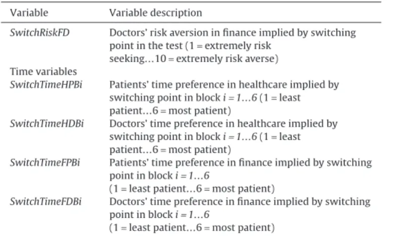
Appendix A (continued)
Variable Variable description
SwitchRiskFD Doctors’ risk aversion in finance implied by switching point in the test (1= extremely risk
seeking…10= extremely risk averse) Time variables
SwitchTimeHPBi Patients’ time preference in healthcare implied by switching point in block i= 1…6 (1 = least patient…6= most patient)
SwitchTimeHDBi Doctors’ time preference in healthcare implied by switching point in block i= 1…6 (1 = least patient…6= most patient)
SwitchTimeFPBi Patients’ time preference in finance implied by switching point in block i= 1…6
(1= least patient…6 = most patient)
SwitchTimeFDBi Doctors’ time preference in finance implied by switching point in block i= 1…6
(1= least patient…6 = most patient)
* Information obtained only for patients. In order to be consultants in outpa-tient clinics, all doctors must have at least one post-graduate medical specialisation.
Appendix B
Structural estimations for the two subsamples of doctors and patients
Table B1 Estimated risk aversion parameters in healthcare under CRRA for patients and doctors.
Healthcare domain Financial domain Patients Doctors Patients Doctors
s 0.1211** 0.2084** −0.0135 0.3217*** (0.0523) (0.0966) (0.0578) (0.1027) μ 34.5443*** 19.6467** 71.8446*** 12.2540** (8.5544) (8.5086) (20.7588) (5.7425) Observations 2700 603 2700 603 Log pseudo LL −1422.77 −296.93 −1450.75 −305.97 Note: * p< 0.1, ** p < 0.05, ***p < 0.01.
Table B2 Estimated discounting parameters in the healthcare domain under exponential, hyperbolic, and quasi-hyperbolic discounting models.
Healthcare domain Financial domain
Exponential Hyperbolic Quasi-hyperbolic Exponential Hyperbolic Quasi-hyperbolic
(2) Patients μ 0.0036*** 0.0042*** 0.0035*** 0.0044*** 0.0052*** 0.0048*** (0.0002) (0.0003) (0.0003) (0.0003) (0.0004) (0.0004) r 0.0215*** 0.0338*** 0.0233*** 0.0279*** 0.0465*** 0.0225*** (0.0029) (0.0054) (0.0031) (0.0040) (0.0078) (0.0033) b 1.0445*** 0.8829*** (0.0635) (0.0548) Observations 7605 7605 7605 4255 4255 4255 Adj R-squared 0.5525 0.5535 0.5525 0.6290 0.6293 0.6298 (2) Doctors μ 0.0038*** 0.0039*** 0.0036*** 0.0055*** 0.0058*** 0.0057*** (0.0006) (0.0006) (0.0006) (0.0009) (0.0009) (0.0009) r 0.0065*** 0.0087** 0.0071*** 0.0082*** 0.0115*** 0.0077*** (0.0018) (0.0031) (0.0017) (0.0017) (0.0029) (0.0015) B 1.0426*** 0.9685*** (0.1016) (0.0788) Observations 1780 1780 1780 1405 1405 1405 Adj R-squared 0.3878 0.3883 0.3880 0.4313 0.4321 0.4315 Note: * p< 0.1, ** p < 0.05, ***p < 0.01. Appendix: Supplementary material
Supplementary data to this article can be found online at doi:10.1016/j.jhealeco.2016.10.001.
References
Ahlbrecht, M., Weber, M., 1997. An empirical study on intertemporal decision making under risk. Management Science 43, 813–826.
Ainslie, G., 1975. Specious reward: a behavioral theory of impulsiveness and impulse control. Psychological Bulletin 82, 463.
Allison, J.J., Kiefe, C.I., Cook, E.F., Gerrity, M.S., Orav, E.J., Centor, R., 1998. The association of physician attitudes about uncertainty and risk taking with resource use in a Medicare HMO. Medical Decision Making: An International Journal of the Society for Medical Decision Making 18, 320–329.
Anderhub, V., Güth, W., Gneezy, U., Sonsino, D., 2001. On the interaction of risk and time preferences: an experimental study. German Economic Review 2, 239–253. Andersen, S., Harrison, G.W., Lau, M.I., Rutström, E.E., 2008a. Lost in state space: are
preferences stable? International Economic Review 49, 1091–1112.
Andersen, S., Harrison, G.W., Lau, M.I., Rutström, E.E., 2008b. Eliciting risk and time preferences. Econometrica: Journal of the Econometric Society 76, 583–618. doi:10.1111/j.1468-0262.2008.00848.x.
Andersen, S., Harrison, G.W., Lau, M.I., Rutström, E.E., 2010. Behavioral econometrics for psychologists. Journal Of Economic Psychology 31, 553–576.
Andersen, S., Harrison, G.W., Lau, M.I., Rutström, E.E., 2013. Discounting behaviour and the magnitude effect: evidence from a field experiment in Denmark. Economica 80, 670–697. doi:10.1111/ecca.12028.
Andersen, S., Harrison, G.W., Lau, M.I., Rutström, E.E., 2014. Discounting behavior: a reconsideration. European Economic Review 71, 15–33.
Anderson, L.R., Mellor, J.M., 2008. Predicting health behaviors with an experimental measure of risk preference. Journal of Health Economics 27, 1260–1274.
Andreoni, J., Sprenger, C., 2012. Risk preferences are not time preferences. The American Economic Review 102, 3357–3376.
Angeletos, G.-M., Laibson, D., Repetto, A., Tobacman, J., Weinberg, S., 2001. The hyperbolic consumption model: calibration, simulation, and empirical evaluation. Journal of Economic Perspectives: A Journal of the American Economic Association 15, 47–68.
Atanasov, P., Anderson, B.L., Cain, J., Schulkin, J., Dana, J., 2013. Comparing physicians personal prevention practices and their recommendations to patients. Journal for Healthcare Quality doi:10.1111/jhq.12042.
Attema, A.E., 2012. Developments in time preference and their implications for medical decision making. Journal of the Operational Research Society 63, 1388–1399.
Attema, A.E., Bleichrodt, H., Rohde, K.I., Wakker, P.P., 2010. Time-tradeoff sequences for analyzing discounting and time inconsistency. Management Science 56, 2015–2030.
Axon, R.N., Bradford, W.D., Egan, B.M., 2009. The role of individual time preferences in health behaviors among hypertensive adults: a pilot study. Journal of the American Society of Hypertension 3, 35–41.
Barseghyan, L., Prince, J., Teitelbaum, J.C., 2011. Are risk preferences stable across contexts? Evidence from insurance data. The American Economic Review 101, 591–631.
Barsky, R.B., Kimball, M.S., Juster, F.T., Shapiro, M.D., 1995. Preference parameters and behavioral heterogeneity: an experimental approach in the health and retirement survey. National Bureau of Economic Research 112, 537–579. Battalio, R.C., Kagel, J.H., Jiranyakul, K., 1990. Testing between alternative models of
choice under uncertainty: some initial results. Journal of Risk and Uncertainty 3, 25–50.
Becker, G.S., Mulligan, C.B., 1997. The endogenous determination of time preference. The Quarterly Journal of Economics 112, 729–758.
Beisswanger, A.H., Stone, E.R., Hupp, J.M., Allgaier, L., 2003. Risk taking in relationships: differences in deciding for oneself versus for a friend. Basic and Applied Social Psychology 25, 121–135.
Benhabib, J., Bisin, A., Schotter, A., 2010. Present-bias, quasi-hyperbolic discounting, and fixed costs. Games and Economic Behavior 69, 205–223.